Enhanced Resolution
Land Surface Temperature is no longer sold at 20 m and 100 m resolution. Active contracts remain fully supported through their remaining terms, and the core infrastructure will officially sunset in November 2027. Upon renewal, please contact your Account Executive to transition to our 1000 m product variant or explore other suitable alternatives for your specific use case.
Land Surface Temperature 100 m
Product Specifications
Table 1: LST 100 m product specification
| Data Resource | LST 100 m |
|---|---|
| Source ID | LST-AMSR2_V1.0_100 |
| Version | 1.0 |
| Unit | Kelvin |
| Pixel Size | 0.00089° (±100x100 m) |
| Temporal Resolution | 0° latitude: 205 to 228 observations per overpass time per year 40° latitude: 274 to 292 observations per overpass time per year |
| Overpass Time | 01:30 and 13:30 local solar time |
| Geographical Coverage | Global |
| Data Availability | 2017-07-01 - Present |
| Satellites Used | AMSR-2, Sentinel-2 |
| NRT latency (p90) | 24 hours |
| Archive latency | Within 30 days after creating a subscription |
Asset Properties
Each LST 100 m observation is delivered as a LST data asset (*lst.tif) with metadata provided in a separate quality flag asset (*lst-qf.tif).
Table 2: Asset properties of LST 100 m data resources
| Asset Name | Band Name | Unit | Type | Typical Range | No Data Value | Scale | Format |
|---|---|---|---|---|---|---|---|
| lst | Band 1 | kelvin | UINT16 | 263 - 340 | 65535 | 0.01 | GeoTIFF |
| lst | Band 2 | kelvin | UINT16 | 250 - 360 | 65535 | 0.01 | GeoTIFF |
| lst-qf | Band 1 | unitless | UINT16 | NA | 0 | 1 | GeoTIFF |
You can find below a Python code snippet that converts a temperature from Kelvin to Celsius and Fahrenheit:
def kelvin_to_celsius(kelvin):
    return kelvin - 273.15

def kelvin_to_fahrenheit(kelvin):
    celsius = kelvin - 273.15
    return (celsius * 9/5) + 32
Enhancements Using Optical Data
Land Surface Temperature is also highly variable in space, mainly due to soil properties, topography, agricultural practices, and land cover heterogeneity. Space-borne optical/thermal sensors can help retrieve high-resolution surface parameters. Several studies (Lobell & Asner 2002, Fensholt and Sandholt 2003, Sadeghi et al. 2017, Yue et al. 2019) found that soil and plant water content greatly influences the reflection in the shortwave infrared (SWIR) part of the spectrum. The SWIR, combined with the Near-Infrared (NIR) reflectance, which is affected by internal leaf structure and leaf dry matter content but not by water content, will enhance the LST retrieval from reflectances.
We produce a daily NDSWIR composite using a backward Gaussian weighted distribution. This composite integrates into the downscaling framework by attributing the weight of a brightness temperature to each pixel within the footprint. The output format remains similar to that of the downscaling algorithm without NDSWIR input.
The Sentinel-2 data is extracted from L2A - Bottom of the atmosphere (BOA) - reflectance in the Sentinel-2 dataset documentation.
Input Data
Table 3: List of inputs for LST 100 m production
| Product | Description |
|---|---|
| Brightness Temperature Ka band | AMSR-E and AMSR-2 Level-1B Radiometer Ka band Brightness Temperatures (downloaded from JAXA G-portal in HDF5 format). This Level-1B product provides calibrated estimates of geolocated brightness temperatures at 36.5 GHz with a footprint size of 7x12 km. Data has been available from July 2002 to October 2011 (AMSR-E) and from June 2012 (AMSR-2) up to now with a latency of 12 hours. Detailed information is available here. |
| Brightness Temperature W band | AMSR-E and AMSR-2 Level-1B Radiometer W band Brightness Temperatures (downloaded from JAXA G-portal in HDF5 format). This Level-1B product provides calibrated estimates of geolocated brightness temperatures at 89 GHz with a footprint size of 3x5 km. Data has been available from July 2002 to October 2011 (AMSR-E) and from June 2012 (AMSR-2) up to now with a latency of 12 hours. Detailed information is available here. |
| Reflectances SWIR and NIR | Sentinel-2 Level-2A reflectance data for two bands: SWIR (shortwave infrared around 1610 nm) and NIR (near infrared around 842 nm). |
| Digital Elevation Model | Digital elevation model (DEM) static map based on the Copernicus DEM GLO-90 product covering the full global landmass of the time frame of data acquisition (2011-2015). Detailed information is available in the link. |
| Land Cover Map | Custom global land classification including permanent water bodies based on the Copernicus Global Surface Water Bodies product from PROBA-V. Detailed information is available here |
Validation
The white paper includes a spatial comparison of the Planet 100m LST against Landsat LST. The revisit time of Landsat is low with one observation every 8 days at best, since thermal-based LST is sensitive to cloud cover. The overpass time of Landsat is between 10:00 and 10:25 while Planet LST daytime is at 13:30. Due to the mismatch in observation time, the focus on the analysis is on the relative spatial variability, rather than the absolute comparison.
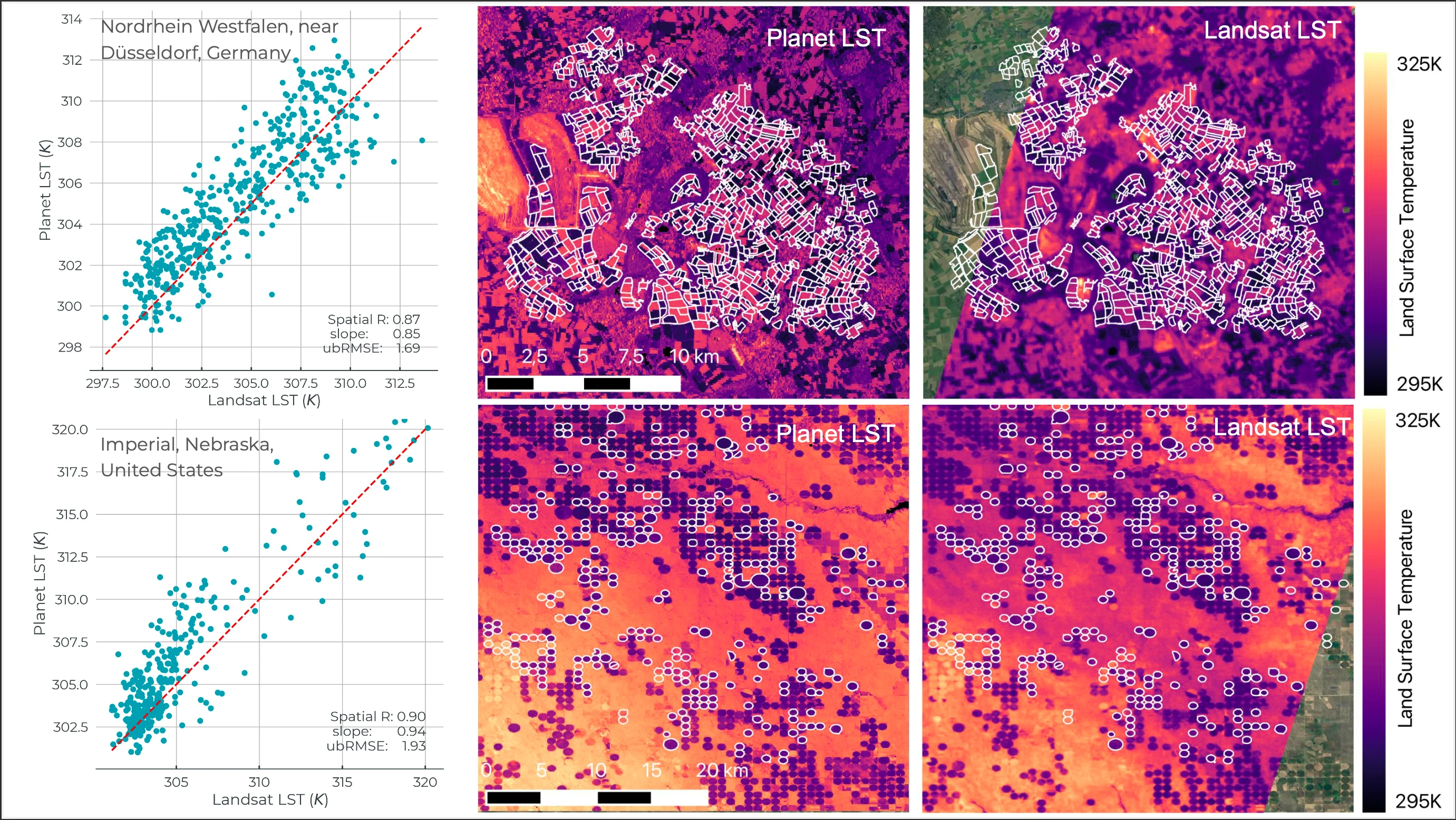
Figure 1: Spatial comparison of 100 m LST compared to Landsat LST. The scatterplot on the left presents a comparison for agricultural fields on single day between Landsat and Planet LST, the right figures are the maps of the day compared. The area of interest are (top) Nordrhein Westfalen, near Düsseldorf in Germany and (bottom) southwest of Imperial, Nebraska, in the United States.
Metadata
Quality flag assets (*lst-qf.tif) provide metadata for each pixel using bitwise flags. Critical flags indicate unreliable data, with corresponding pixels in band 1 of the LST asset (*lst.tif) set to the no data value. The replaced LST value can be found in band 2 of the LST asset. Non-critical flags indicate that the data can be used with caution, taking into account the flag description.
Critical and non-critical flags are described in the tables below. For more information on how to access the quality flag asset, check out subscribing to Planetary Variables.
Table 4: Non-critical flags
| Bit | Flag layer | Description |
|---|---|---|
| 4 | Possible severe precipitation | Part of the footprints touch an area flagged as severe precipitation. |
| 7 | Possible frozen soil | The surface may be frozen. These are pixels with a surface temperature between 263.15 K (-10°C) and 273.15 K (0°C). |
Table 5: Critical flags
| Bit | Flag layer | Description |
|---|---|---|
| 8 | Frozen soil | The surface is considered frozen. Pixels with a temperature below 263.15 K (-10°C). |
| 9 | Severe precipitation | Severe precipitation is detected. |
| 11 | No overpass | The satellite did not pass over. |
| 13 | Instrumental flaws | Unrealistic values due to instrumental flaws. If the brightness temperature at 36.5 GHz V produces values either over 400K or under 0.9 * the water temperature, the data is considered as unrealistic and is removed. |
| 14 | Out of valid range | Land Surface Temperature values are outside the valid range, meaning under 250 K or above 340 K. |
| 15 | Open water | Land Surface Temperature is not defined over water (retrieved from a land cover map). This data is filtered out during the processing of the raw satellite data. |
Here is a Python script to convert a quality flag pixel value into a list of corresponding quality flags. Note that one pixel may have multiple flags applied to it.
# lst_quality_flags.py

import argparse

LST_QUALITY_FLAGS = {
    4: "Possible severe precipitation",
    7: "Possible frozen soil",
    8: "Frozen Soil (critical flag)",
    9: "Severe precipitation (critical flag)",
    11: "No overpass (critical flag)",
    13: "Instrumental flaws (critical flag)",
    14: "Out of valid range (critical flag)",
    15: "Open water (critical flag)",
}


def convert_to_quality_flags(decimal_value: int) -> list[str]:
    binary_string = format(decimal_value, "016b")
    reversed_binary_string = binary_string[::-1]
    return [
        f"{i}. {LST_QUALITY_FLAGS.get(i, 'Unused flag')}"
        for i, bit in enumerate(reversed_binary_string, start=1) if bit == "1"
    ]


if __name__ == "__main__":
    parser = argparse.ArgumentParser(description="Convert a decimal value to quality flags.")
    parser.add_argument("decimal_value", type=int, help="The decimal value to convert.")
    args = parser.parse_args()

    flags = convert_to_quality_flags(args.decimal_value)
    print(*flags, sep="\n")
that you can call as follows, using value 8512 as example:
> python lst_quality_flags.py 8512
7. Possible frozen Soil
9. Severe precipitation (critical flag)
14. Out of valid range (critical flag)
Other Limitations
- Persistent cloud cover in highly dynamic landscape can decrease the downscaling method accuracy due to the optical observations by Sentinel-2 that are used for the LST 100 m products.
Frequently Asked Questions
What is the difference between the LST 100 m and 1000 m products?
Our LST 1000 m product is based on our patented disaggregation method where we make optimum use of the overlapping satellite footprints to refine the resolution from 36 km to 1 km. The LST 100 m product also uses the NIR and SWIR band from Sentinel-2 to add more spatial constraints to our disaggregation method.
What about cloud cover?
The microwave part of the observations is not hindered by cloud cover. However, for downscaling to 100 m, we rely on near-infrared and shortwave infrared data that are sensitive to cloud cover. As such, there will be regions that will show artifacts in the 100 m data due to long periods with clouds. For all regions with > 70% cloud cover data should only be delivered to clients after a manual inspection (100 m only). This also means that the 100 m is less suitable for monitoring high temporal frequency changes (at the small scale) in cloudy regions.
Land Surface Temperature 20 m
Product Specifications
Table 6: LST 20 m product specification
| Data Resource | LST 20 m |
|---|---|
| Source ID | LST-field_V1.0_20 |
| Version | 1.0 |
| Unit | Kelvin |
| Pixel Size | 20 m |
| Temporal Resolution | 0° latitude: 205 to 228 observations per overpass time per year 40° latitude: 274 to 292 observations per overpass time per year |
| Overpass Time | 01:30 and 13:30 local solar time |
| Geographical Coverage | Global |
| Data Availability | 2018-01-01 - Present |
| Satellites Used | AMSR-2, Sentinel-2 |
| NRT latency (p90) | 24 hours |
| Archive latency | Within 30 days after creating a subscription |
Asset Properties
LST 20 m is field-based: each observation is delivered as a single-band asset with metadata embedded in the GeoTIFF.
Table 7: Asset properties of LST 20 m data resources
| Asset Name | Band Name | Unit | Type | Typical Range | No Data Value | Scale | Format |
|---|---|---|---|---|---|---|---|
| lst | Band 1 | kelvin | UINT16 | 263-340 | 65535 | 0.01 | GeoTIFF |
Input Data
Table 8: List of inputs for LST 20 m production
| Product | Description |
|---|---|
| Brightness Temperature Ka band | AMSR-E and AMSR-2 Level-1B Radiometer Ka band Brightness Temperatures (downloaded from JAXA G-portal in HDF5 format). This Level-1B product provides calibrated estimates of geolocated brightness temperatures at 36.5 GHz with a footprint size of 7x12 km. Data has been available from July 2002 to October 2011 (AMSR-E) and from June 2012 (AMSR-2) up to now with a latency of 12 hours. Detailed information is available here. |
| Brightness Temperature W band | AMSR-E and AMSR-2 Level-1B Radiometer W band Brightness Temperatures (downloaded from JAXA G-portal in HDF5 format). This Level-1B product provides calibrated estimates of geolocated brightness temperatures at 89 GHz with a footprint size of 3x5 km. Data has been available from July 2002 to October 2011 (AMSR-E) and from June 2012 (AMSR-2) up to now with a latency of 12 hours. Detailed information is available here. |
| Reflectances SWIR and NIR | Sentinel-2 Level-2A reflectance data for two bands: SWIR (shortwave infrared around 1610 nm) and NIR (near infrared around 842 nm). |
| Digital Elevation Model | Digital elevation model (DEM) static map based on the Copernicus DEM GLO-90 product covering the full global landmass of the time frame of data acquisition (2011-2015). Detailed information is available in the link. |
| Land Cover Map | Custom global land classification including permanent water bodies based on the Copernicus Global Surface Water Bodies product from PROBA-V. Detailed information is available here |
Metadata
Metadata embedded in the GeoTIFF contains information about the quality of the observation. For example:
Table 9: Metadata fields of LST 20 m data resources
| Field | Type | Description | Example |
|---|---|---|---|
PRODUCT_VERSION | String | Version identifier for the product specification | v1 |
SOFTWARE_VERSION | String | Version of the fbsl software that generated the output | 0.4.1 |
INPUT_ASSETS | String | Comma-separated list of input data sources used | NDSWIR_STATS,NDSWIR_RASTER,KA_V_DESC_STATS |
LAST_NDSWIR_DATE | String (ISO date) | Date of the last NDSWIR (Sentinel-2) observation with full coverage | 2024-01-19 |
LAST_NDSWIR_COV | String (fraction) | Coverage fraction of the last NDSWIR observation used | 0.85 (= 85% coverage) |
QUALITY | String | Overall quality assessment: HIGH if valid coverage > 80%, otherwise LOW | HIGH or LOW |
INVALID_RANGE_COV | String (fraction) | Fraction of pixels outside valid LST range (250-340 K) | 0.02 (= 2% invalid) |