Technical Specification

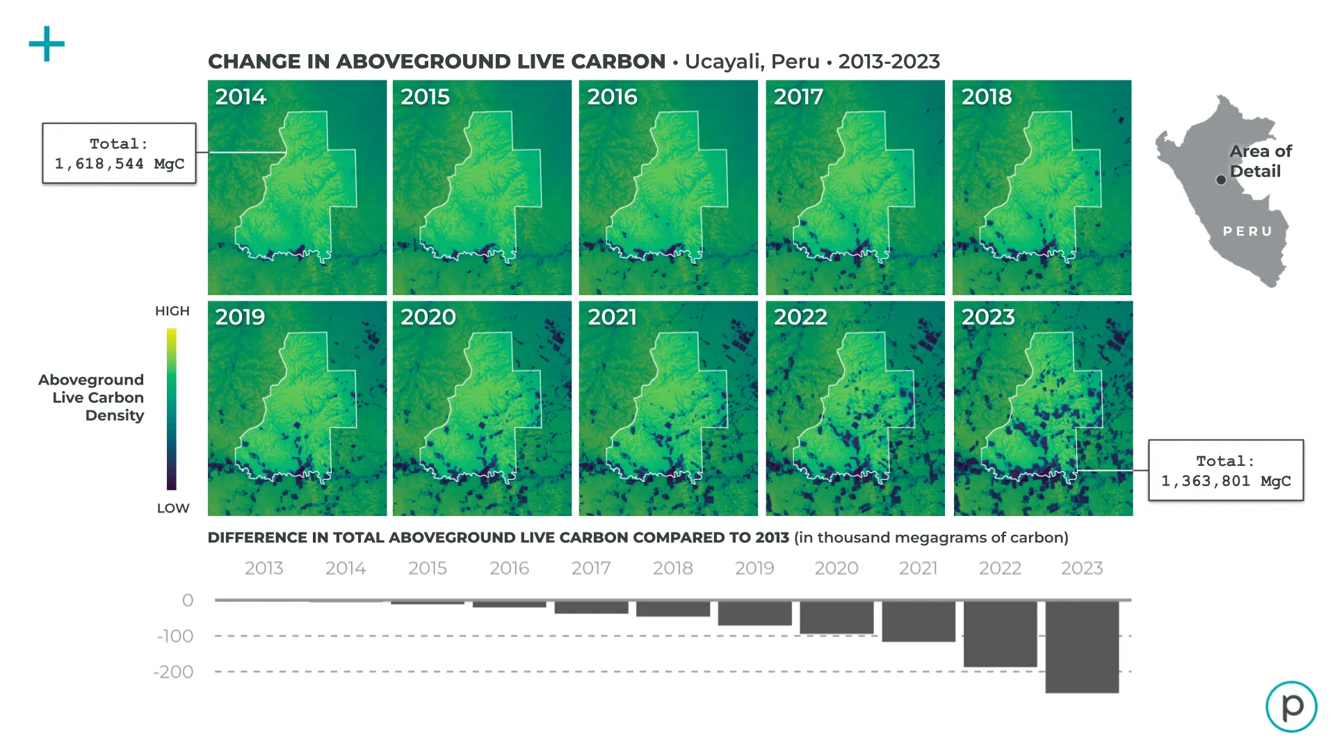
Figure 1: Changes in total aboveground carbon stocks over a simulated forest carbon project boundary in Ucayali, Peru..

This document describes the Planet Forest Carbon Diligence product. It is intended for users of geospatial data interested in working with Forest Carbon Diligence, which estimates aboveground carbon density, canopy height, and canopy cover.

Planet’s Forest Carbon Diligence products quantify—globally and annually—how much carbon is stored in trees, the area occupied by trees, and how tall they are. This is done using cutting edge machine learning models that fuse a rich archive of historical satellite observations with high quality, laser-derived reference data. Modeling benchmarks include an extensive archive of high resolution airborne LiDAR data for training and evaluating the height and cover models, and a global carbon dataset derived from two spaceborne LiDAR missions.

This novel approach builds on decades of open data and open science, and was designed to maximize accuracy, transparency, and trust based on well-known standards.

Mapping and monitoring forest carbon dynamics comes with uncertainty. Forest Carbon Diligence embraces uncertainty by reporting multiple pixel-level uncertainty metrics, including observation quality scores and prediction intervals for each dataset, each designed to support uncertainty propagation into user workflows.

Jurisdictional and voluntary carbon monitoring programs require high quality, accessible, and globally consistent data on the state of the world’s forests, and how they are changing. The Forest Carbon Diligence products were designed to support these needs. Planet is committed to transparency and open science, and has published a full methods and validation report describing this product (Anderson et al., 2025).

The features of Planet’s Forest Carbon Diligence data:

• A multi-year, GEDI-like forest carbon data product with wall-to-wall spatial coverage.
• 12-year series quantifying annual patterns of aboveground carbon density, canopy cover and canopy height.
• Full global coverage of the terrestrial biosphere at 30m resolution.
• All models calibrated and evaluated with high quality reference data.
  • >2 million km2 of airborne LiDAR used to train canopy cover and canopy height models.
  • >80 million spaceborne LiDAR (GEDI, ICESat-2) samples used to train aboveground carbon model.
• Novel cloud masking, pixel selection, multi-sensor fusion, and temporal harmonization techniques developed to minimize year-over-year measurement variability.
• Calibrated, pixel-level prediction intervals support uncertainty propagation to downstream analyses.
• Day-of-measurement and satellite data quality scores provide insights into prediction timing and quality.
• GEDI-based model calibration enables independent validation of our product and simplifies intercomparison with a well-known global standard.

Product Specifications

Table 1: Forest Carbon Diligence product specification

Specification	Value
Metrics	Canopy cover, canopy height, aboveground carbon density
Spatial extent	Global land mass > -60S and < 75N, excluding ice sheets
Spatial resolution	0.00025° (± 30 x 30 m)
Temporal extent	2013 - Present.
Temporal resolution	Annual
Temporal period	Jan 01 - Dec 31.

Canopy cover quantifies the percentage of area occupied by trees within a pixel, where a tree is defined as vegetation 5 meters or taller. This metric will be most sensitive to tree clearing events like timber harvest or deforestation, but is also sensitive to seasonal leaf-on variation and to drought.

Canopy height quantifies the average stand height of trees within each pixel. Because this is a spatial average over a moderate resolution, the modeled height values are shorter than the tallest individual tree within a pixel.

Aboveground carbon density quantifies the expected density of carbon stored in woody biomass across the landscape, measured in mass per area (megagrams of carbon per hectare). It is not a direct estimate of the total carbon in that pixel, as the spatial resolution of each pixel is less than one hectare. To estimate total carbon in a pixel, users should normalize these values to account for the size of each pixel, or average the density values to 1 hectare in an equal area projection.

Asset Properties

This tables specifies the properties of the data assets delivered by the Planet Subscriptions API.

Table 2: Forest Carbon Diligence data resource properties

Metric	Asset Name	Units	Type	Typical Range	No Data Value	Band Count
Canopy Cover	cc	%	UINT8	0 - 100	255	1
Canopy Height	ch	m	UINT8	0 - 50	255	1
Aboveground Carbon Density	acd	Mg/ha	INT16	0 - 300	32767	1
CC Uncertainty	cc-uc	%	UINT8	0 - 100	255	2
CH Uncertainty	ch-uc	m	UINT8	0 - 80	255	2
ACD Uncertainty	acd-uc	Mg/ha	INT16	0 - 400	32767	2
CC Change Detection	cc-change	n/a	UINT8	0 - 2	255	1
CH Change Detection	ch-change	n/a	UINT8	0 - 2	255	1
Quality Flags	acd-qa	n/a	UINT8	0 - 224	255	1
Day of Year	acd-doy	day	INT16	0 - 366	32767	1

The cc, ch, and acd assets contain the predicted values of canopy cover, canopy height, and aboveground carbon density in their natural units. Quality flag and day of year data are provided for all metrics (for example, cc-qa, ch-qa, acd-qa). They are only listed once in the table because they contain duplicate information across metrics.

Uncertainty Bounds

Table 3. Uncertainty band descriptions

Uncertainty Band	Description
Q05 (band 1)	Lower prediction bound (5th percentile)
Q95 (band 2)	Upper prediction bound (95th percentile)

Uncertainty data are provided as calibrated 90% prediction intervals for each pixel in each year. These values are provided in the same units as their respective reference data. In other words, the pixel values and units are consistent between ACD and ACD-UC, between CC and CC-UC, and between CH and CH-UC.

Change Assets

Table 4. Change detection asset pixel values

Pixel Value	Description
0	No change observed
1	Fast change observed, such as deforestation or wildfire disturbance
2	Slow change observed, such as reforestation or natural forest growth

The cc-change and ch-change assets classify annual changes that occur. These are the product of a time series model, which estimates whether a pixel experiences no change, fast change, or slow change from year to year.

Quality Flags

Table 5. QA pixel values

Pixel Value	Description
0-100	Estimated observation quality. Low values indicate low quality observations, like hazy, cloudy, or off-season measurements. High values indicate high quality observations, like clear, cloud-free measurements captured during peak greenness.
213-214	Year of closest available measurement. Some parts of the world experience persistent cloud cover or haze year-round, resulting in 0 valid measurements in a year. In these cases, the nearest-in- time clear observation is used. For example, 213 refers to 2013, and 222 refers to 2022

Planet provides pixel-level QA data to indicate the relative quality of each pixel’s satellite data observation. These values are provided to diagnose whether observed changes might be the result of low quality measurements.

Day of Year

Table 6. DOY pixel values

Pixel Value	Description
0	No measurement available. These primarily occur over water bodies where data are not provided.
1-366	Julian day of the measurement. If this pixel has been filled with a nearest-in-time observation from a nearby year, the day of that year’s observation is reported.

Day of year pixel values encode the calendar day of the satellite observation. Since the number and quality of observations vary with the number of cloud-free observations, differences in observation dates between adjacent pixels can be large. This information can indicate seasonal differences between observations. It can also indicate whether an observation occurred prior to or following a disturbance.

Input Data

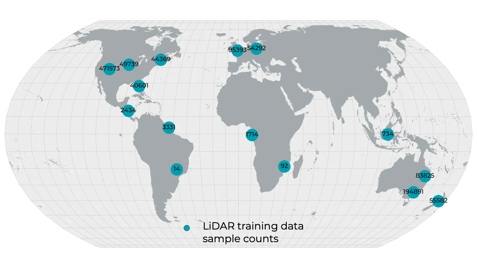
Figure 2: Extent and count of the airborne LiDAR data used for model training and evaluation.

The Forest Carbon Diligence product uses multi-source, multi-scale earth observations data from a series of publicly available resources and derivative data products. The metrics derived from airborne and spaceborne LiDAR were treated as response variables, which were modeled using optical, radar, and derived feature data.

Table 7: List of inputs for Forest Carbon Diligence production

Product	Description
Airborne LiDAR	Point cloud data processed to canopy height and canopy cover rasters at 1m resolution then resampled to 30m resolution for model training
Spaceborne LiDAR	GEDI L4A and ICESat-2 ATLAS encode modeled estimates of aboveground biomass density. GEDI provides coverage over mid latitudes (<51.6 N, >51.6 S) and ICESat-2 provides coverage for high latitudes (>44.4 N)
Surface Reflectance	The full scene archive of Landsat-8, Landsat-9, and Sentinel-2 were processed to BRDF-adjusted surface reflectance using FORCE (Frantz 2019). These scenes were masked for clouds, shadows, and haze and composited into annual best-available-pixel mosaics
L-band RaDAR backscatter	L-band SAR mosaics from ALOS PALSAR-2. Both HH and HV polarizations were downloaded for each year. No rescaling or normalization was applied to these data
Wood density	Wood density estimates were used as features in the canopy height and canopy cover models. These estimates encode coarse scale (~1 km) biogeographic information that might inform the mapping from remote sensing data to forest structural traits
Digital Elevation Model (DEM)	Copernicus GLO-30 DEM are used for most of the global landmass, ALOS AW3D30 is used where GLO-30 does not provide data

Methods

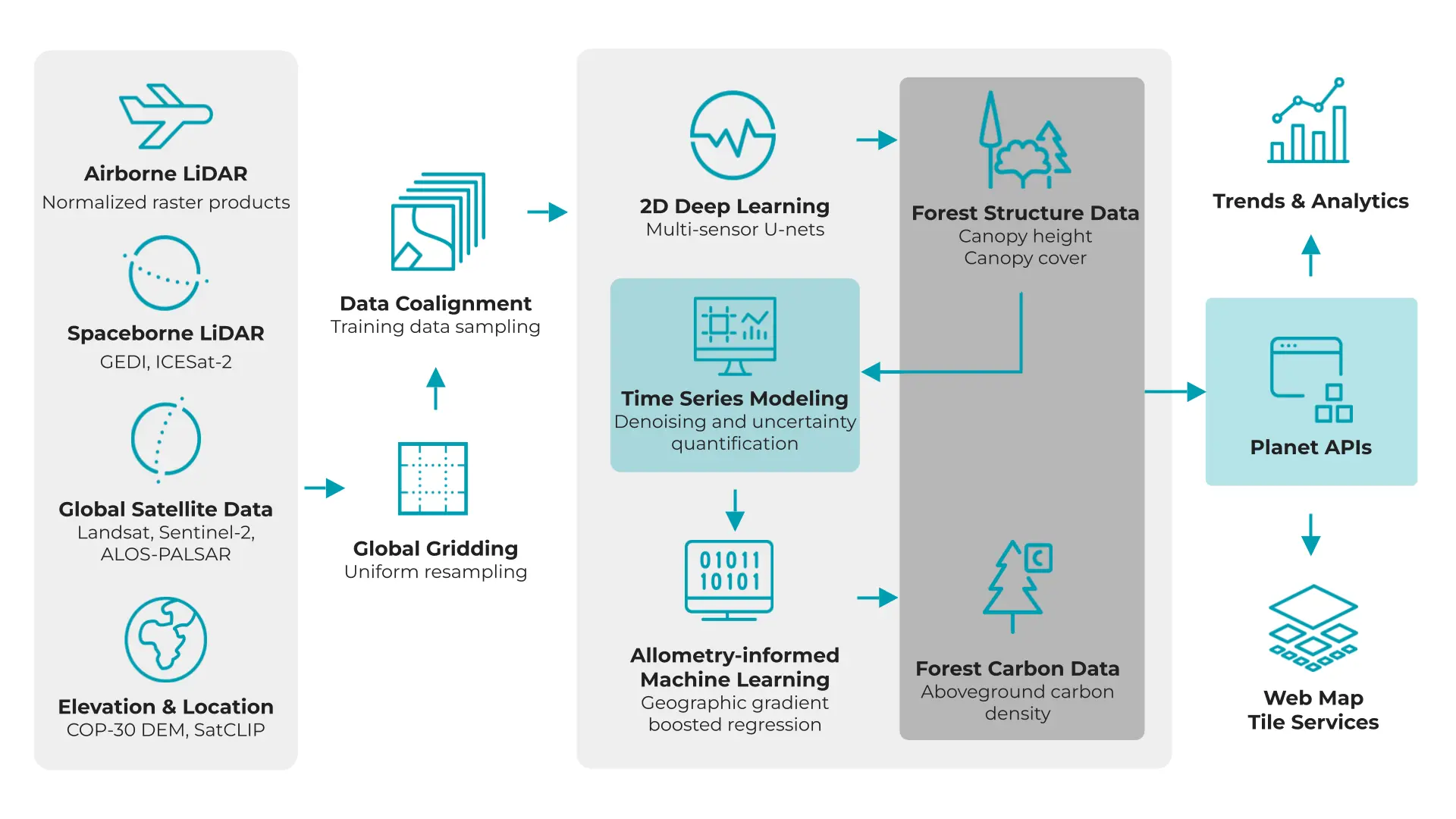
Figure 3: Workflow diagram for Forest Carbon Diligence illustrating the flow of data for delivery.

The Forest Carbon Diligence products were created using multi-scale, publicly available EO data. These datasets were modeled in a stepwise process to balance the strengths and limitations of each dataset. Fully detailed methods, validation results, and data sources are described in Anderson et al., 2025.

Airborne LiDAR Data

Point cloud data were downloaded from a series of open data platforms, reprojected to a consistent coordinate system (EPSG:6933) and normalized in the Z dimension to height above ground. Ground point classifications provided in the source data were used for normalization. Buildings, bridges, noise, and other non-vegetation classes were removed from processing using the point classifications provided in the source data, when present. For datasets with no prior classifications, custom building and noise classifiers were used. Canopy height and canopy cover were rasterized from the normalized point cloud data at 1 m native resolution. Overall, 2,234,400 km2 of LiDAR data were processed and extracted for model training and evaluation (Fig. 2).

Canopy height (m) was calculated as the tallest point within each grid cell using a modified pit-free canopy height model algorithm (Khosravipour et al. 2014). This is not restricted to trees as there is no height or size threshold for inclusion; the height of the tallest vegetation at each cell is recorded, be it grass, shrub, or tree.

Canopy cover (%), also referred to as canopy density, is calculated as the number of LiDAR returns 5m and above divided by the total number of returns within each grid cell. This threshold tracks overstory vegetation cover, and can be interpreted as a proxy for canopy closure; cover increases in proportion to overstory foliage volumes. It can be interpreted as the complement to canopy gap fraction (CC = 1 − GF; Coomes et al. 2017).

Average resampling to a lower resolution reduces the range of observed canopy height values to approximately 0-40 m. Average resampling was selected because this implicitly weights pixel-level tree height measurements by crown diameter, and the combination of these variables is correlated with aboveground biomass across ecosystems (Jucker et al. 2018).

Spaceborne LiDAR Data

AGBD estimates from GEDI v2.1 (Dubayah et al. 2022) and ICESat-2 ATLAS (Montesano et al. 2024) were downloaded, merged, and organized into a harmonized dataset using a global equal area tile grid (see Gridding and Sampling). These two sources of AGBD estimates are complementary, with overlap, as GEDI provides coverage over mid latitudes (<51.6 N, >51.6 S) and ICESat-2 provides coverage for high latitudes (>44.4 N).

A series of quality filters were applied to the GEDI observations, selecting samples from power beams, collected at night, excluding steep slopes, and excluding orbits with high geolocation error. ICESat-2 data were filtered by the data providers. Additional outlier detection was applied to both GEDI and ICESat-2 observations, which identified and removed anomalously tall RH98 observations, particularly over sparsely arbored areas.

Overall, 586 million GEDI observations and 15 million ICESat-2 observations were retained after filtering (30% and 99% of the original observations, respectively). A final spatially balanced random sampling step yielded 81.6 million waveforms to be used for training and evaluation, reducing bias in oversampled regions and better approximating a geographically uniform random sample (Meyer and Pebesma 2022).

Surface Reflectance

Multispectral surface reflectance data provided 6 of the 9 feature bands used for the forest structure models. Surface reflectance is sensitive to patterns of vegetation growth and structure, with optical variation driven by a combination of leaf-level and canopy-level growth and structure metrics (Jordan 1969, Knipling 1970, Asner 1998, Dalagnol et al. 2023).

The full scene archives of Landsat-8, Landsat-9, Sentinel-2A and Sentinel-2B were downloaded from public cloud storage. Each scene was processed to nadir BRDF-adjusted surface reflectance using the FORCE atmospheric correction and normalization algorithm (Frantz 2019). FORCE produces a scene-level QA mask classifying cloud, shadow, haze, water, and snow using a modified version of FMask (Qiu et al. 2019, Skakun et al. 2022). Sentinel-2 scenes were average resampled to match Landsat’s resolution. To reduce false negative cloud detections, a custom cloud and shadow mask was applied to update each scene’s QA mask. Only the six bands shared across instruments were retained: [B, G, R, NIR, SWIR-1, SWIR-2].

Annual surface reflectance mosaics were created beginning in 2013, which marks the launch of Landsat-8 (Roy et al. 2014). These mosaics were created using a custom best-available-pixel compositing method, adapted from White et al. 2014. Best-pixel methods show strong temporal consistency compared to percentile-based composites, though this may come at the expense of radiometric uniformity (Matasci et al. 2018).

The following quality metrics were used:

• Haze score. Aerosol optical depth (AOD) estimates from FORCE were used to indicate haze. Quality scores were set inversely proportional to AOD scores, where lower AOD indicates a higher quality score.
• Distance to cloud score. Some cloud edges are not correctly classified by the strict cloud mask, so the euclidean distance to each cloudy pixel downranked pixels close to cloud detections.
• Solar zenith angle score. Sun-sensor geometry is the primary driver of variation in surface reflectance, leading to large differences in observation conditions over the year, especially at high or low latitudes. Solar zenith angle was used as a quality metric to prioritize scenes collected during well-lit observation conditions, which improves retrieval of vegetation structural information (Dalagnol et al. 2023).
• Day of year score. Because vegetation varies throughout the year in response to seasonal change, a day of year score was defined to prioritize spring measurements.
• Sensor score. Landsat scenes were ranked lower than Sentinel-2 scenes because the Sentinel-2 cloud mask reports higher precision scores and includes fewer false negatives (Frantz et al. 2018).

The pixel composite method addressed three needs.

First was to maximize consistency in the observation conditions for each pixel. The compositor included scoring factors based on sun angle, expected time of peak greenness, distance to clouds, aerosol density, and instrument type. Pixel quality increased as solar elevation increased, at times closest to peak greenness, as aerosol content decreased, and for Sentinel-2 observations over Landsat-8/9 observations.

The second goal of the compositor was to provide a quantitative flag for observation quality. Pixel quality scores provide information regarding the expected reliability of each observation, allowing users to filter or weight observations based on pixel quality.

Finally, the compositor records the Julian day of the best pixel, providing a timestamp for when each observation occurred.

L-Band RaDAR, Wood Density, and Elevation Data

Annual, radiometrically balanced L-band Synthetic Aperture Radar mosaics from ALOS-PALSAR-2 were downloaded from JAXA’s HTTP server. The HH and HV polarizations comprise 2 of the 9 total predictor bands used for the canopy cover and canopy height models. Active microwave measurements are directly sensitive to aboveground plant water content, and L-Band measurements in particular are typically sensitive to the water content of large, woody biomass components, like tree trunks and branches, indirectly measuring key components of stand-level vegetation structure (Shimada et al. 2011, Konings et al. 2019). The HH/HV polarization data were not transformed, save for data type and nodata value harmonization across datasets.

Global estimates of wood density were generated at a 1 km resolution via gradient boosted regression of field-observed wood density against principal-component normalized WorldClim and Soilgrids data. This is the final predictor used for the canopy cover and canopy height models, and was included as an index of plant community biogeography to identify non-stationary relationships between target and predictor variables by vegetation type (Hawkins 2011). In total 396,694 field inventory plots were used for training, including data from national forest inventories, ecological monitoring networks, research consortiums, and open data repositories.

Elevation data were used as a predictor for the aboveground carbon density model. This allowed the model to learn nonstationary carbon-topography relationships at local and regional scales, capturing fine-scale topoedaphic drivers of carbon storage in slopes and floodplains (Marvin et al. 2014, Taylor et al. 2015, Jucker et al. 2018) and along elevation gradients (Asner et al. 2014, Mahli et al. 2017, Marifatul Haq et al. 2022). Elevation data were primarily sourced from the Global 30 m Copernicus Digital Elevation Model (ESA 2022). Since this dataset does not include data over Armenia and Azerbaijan, values for those countries were derived from the ALOS World-3D DEM (Tadono et al. 2014).

Canopy Height and Canopy Cover Models

Deep learning regression models were trained to predict mean canopy height and canopy cover independently at 30 m nominal resolution using surface reflectance, HH/VV backscatter, and wood density data as feature variables and airborne LiDAR as response variables. The feature and response variables were normalized to a common range using robust scaling. U-Net convolutional neural network architectures were selected for their robust performance in mapping ecological patterns from EO data (Ronneberger et al. 2015, Broderick et al. 2019, Kattenborn et al. 2021, Wagner et al. 2024).

Training data were generated by randomly sampling 128x128 pixel tiles from regions with coincident airborne LiDAR data. The year of the satellite data closest to the LiDAR acquisition was used for temporal matching. A total of 1,099,559 samples were extracted at an average sample density of 2 points per square kilometer using uniform random geographic sampling. Samples were randomly assigned to training/validation sets (67%) or interval calibration/testing (33%) sets. The training/validation data were then randomly split 70/30, and the interval calibration/testing data were randomly split 20/80.

Training data were used to fit model parameters. Validation data were used to approximate out of sample predictive performance during training. Interval calibration data were used in conformal inference to generate 90% prediction intervals. Test data were used to evaluate predictive performance.

Time Series Model

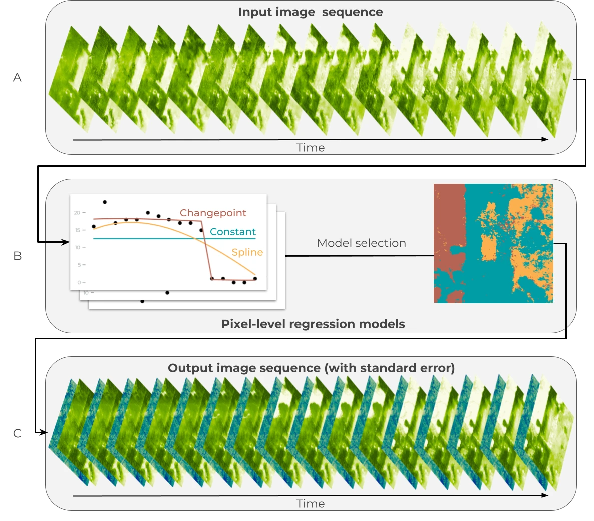
Figure 4: Statistical model for estimating canopy height and canopy cover over time. (A) A time series is generated from the raw predictions for times t=1, … T. (B) Three models are fit for each pixel: a constant model to represent the mean (blue), a changepoint model to represent sudden change (red), and a spline model to represent gradual change (orange). (C) The preferred model for each pixel is used to generate expected values (green) and standard errors (blue) for each time step.

The Diligence U-net models predict height and cover independently for each year, and these predictions contain non-structural variation related to phenology, illumination, and sensor calibration. This residual prediction variation was minimized using statistical models. For each pixel, three models were fit (Fig. 4):

• A constant-in-time model, which represents stability over time
• A spline model, which represents gradual change
• A changepoint model, which represents fast change

The constant model assumes that all variation in predictions is due to noise, and assumes height or cover remains stable over time or when changes are minimal relative to prediction noise (for example, slow growth that is not detectable). The spline and changepoint models capture slow and fast changes, respectively. Regularized B-splines are used to estimate non-linear trends, while the changepoint model included an additional discrete change point parameter at the timestep with the greatest change in predicted height or cover.

The preferred model for each pixel was selected using Akaike's Information Criteria (AIC). An additional heuristic was applied to reduce noise: if the coefficient of variation (CV) over time for the selected model's predictions is below a threshold, the constant-in-time model was selected. This CV threshold is a hyperparameter tuned alongside the AIC threshold. Once a preferred model was selected for each pixel, predictions were generated and the standard errors were used to quantify pixel-level uncertainty for height and cover.

Time series outputs for each year are provided as an additional data asset, with categorical classes mapping no change, fast change, and gradual change (classes [0, 1, 2], respectively).

Canopy Height and Canopy Cover Uncertainty

Standard errors from the height and cover time series models were used to construct 90% prediction intervals:

$[y_{pred} - \widehat{q} \cdot \sigma_{pred}, y_{pred} + \widehat{q} \cdot \sigma_{pred}]$

where $y_{pred}$ is a predicted value from the time series model, $\sigma_{pred}$ is the standard error of the prediction, and $\widehat{q}$ is a parameter estimated using withheld data via split conformal inference.

Split conformal inference uses disjoint partitions of a dataset to produce well-calibrated prediction intervals. These are 90% prediction intervals that contain the true value approximately 90% of the time (Angelopolous and Bates 2021).

A calibration dataset is used to estimate $\widehat{q}$, a scalar quantity that determines the width of the interval relative to the standard error to achieve 90% coverage. After generating predictions with $\widehat{q}$, empirical interval coverage is quantified on a spatially non-overlapping test set. Test set coverage was 90.0% for canopy cover and 90.1% for canopy height.

Aboveground Carbon Density Model

Light gradient-boosting machine (LightGBM) regression models were trained to predict GEDI L4A and ICESat-2 aboveground biomass as a function of predicted mean canopy height, canopy cover, elevation, and location. Location data were encoded using SatCLIP positional embeddings (Klemmer et al. 2023).

The relationships between forest structure and aboveground biomass vary across plant communities, biomes, and topographic gradients, and these shifting relationships are explicitly encoded in the GEDI L4A biomass algorithm (Jucker et al. 2018, Duncanson et al. 2022, Kellner et al. 2023, Ma et al. 2023). Incorporating location features into a tree-based regression model can represent multiple nonstationary relationships: specifically, between predictors and both the mean biomass density and its associated uncertainty (Hawkins, 2011).

10-fold spatial cross validation was used to assess out-of-sample predictive performance, where each of the 7,408 tiles containing GEDI or ICESat-2 biomass estimates were assigned to one of ten partitions (Meyer and Pebesma 2022). For each fold, 5% of the training data were randomly withheld for uncertainty calibration.

Model hyperparameters were evaluated using Bayesian optimization of cross-validation RMSE on a random 25% of data. The number of trees, the leaves in each tree, as well as both L1 and L2 regularization were modified. Final hyperparameter selection was also informed by visual inspection of predictions and external intercomparisons.

Uncertainty was quantified via conformalized quantile regression, which yielded 90% prediction intervals where interval widths vary nonlinearly as a function of model predictors (Romano et al. 2019). In particular, LightGBM quantile regressors were fit to estimate the 5% and 95% quantiles, then conformalized to obtain prediction intervals with strong coverage guarantees on unseen data (Angelopolous and Bates 2021).

Conformalized quantile regression was selected for two reasons. First, nonstationary errors were expected to vary nonlinearly as a function of model inputs, including location. Second, reported uncertainties for footprint-level biomass estimates generally underestimate on-orbit uncertainties that arise from error in relative height estimates (Duncanson et al. 2022). Prediction intervals from conformal inference, in contrast, reflect the empirical distribution of on-orbit data, propagating both measurement- and model-based uncertainty.

Finally, aboveground biomass density is converted to aboveground carbon density by multiplying by the global mean carbon concentration: 0.476 (Martin et al. 2018).

Post Processing

Estimates of height, cover, and aboveground carbon density were minimally post-processed using simple heuristics. To reduce low noise, canopy cover values < 5% were set to zero. If canopy cover was zero at both the beginning and the end of the time series, then all annual cover values were set to zero. Where canopy cover was estimated as zero, canopy height and aboveground carbon density were also set to zero.

Data Quality

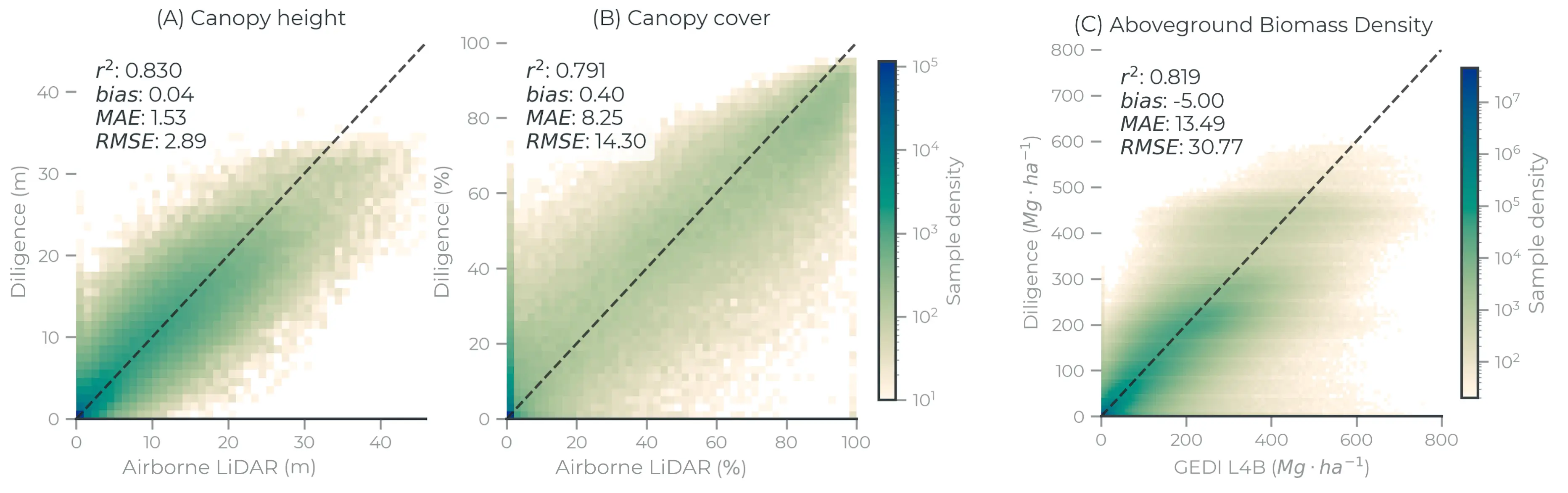
Figure 5: Model performance evaluated on withheld samples (n=360,853 tiles) for (A) mean canopy height and (B) canopy cover at 30 m resolution. Performance metrics were computed using the full withheld datasets but the plots were subset to 1 million random samples for visualization. (C) Aboveground biomass model performance evaluated against GEDI L4B data at 1 km resolution. A minimum of 20 points per grid cell were used for visualization.

The evaluation framework for this product includes two primary components: withheld data evaluation, and intercomparison. Withheld data evaluation refers to comparisons with samples of directly comparable observations, like airborne or spaceborne LiDAR data. Intercomparison evaluates modeled Diligence estimates against modeled estimates from external sources, like field plots and third party satellite observations. This distinction is particularly important when comparing carbon density or biomass density data. To fully evaluate the quality of this product, we hihgly recommend reading the full methods and validation report describing this product (Anderson et al., 2025).

Airborne LiDAR Comparison

The canopy height model has a root mean squared error (RMSE) of $2.9\ m$, mean absolute error (MAE) of $1.5\ m$, bias of $0.04\ m$, and an $r^2$ value of $0.83$ (Fig. 5A). The canopy cover model has $RMSE = 14.3$, $MAE = 8.25$, $bias = 0.4$, and $r^2 = 0.79$ (Fig. 5B).

GEDI L4A and ICESat-2 Comparison

Based on 10-fold geographic cross validation, the aboveground biomass model has a mean RMSE of $55.27\ Mg \cdot ha^{-1}\ (sd = 2.18)$, mean MAE of $24.2\ Mg \cdot ha^{-1}\ (sd = 0.87)$, mean bias of $-0.06\ (sd = 0.39)$, and a mean $r^2$ value of $0.638\ (sd = 0.01)$. Uncertainty estimation showed empirical interval coverage on withheld data was 92.07%, and the mean interval width is $100.9\ Mg \cdot ha^{-1}$.

GEDI L4B Comparison

Comparing mean aboveground biomass density at a 1 km scale against GEDI L4B — a product that statistically aggregates L4A footprints and is not independent from the training data — reports model performance scores of $RMSE = 30.77\ Mg \cdot ha^{-1}$, $MAE = 13.49 Mg \cdot ha^{-1}$, $bias = -5.0 Mg \cdot ha^{-1}$, and $r^2 = 0.819$ (Fig. 5C). Further resampling to 1 degree grid cells shows strong agreement between Diligence and GEDI L4B ($r=0.98$, $bias=-5.0$, $RMSE=14.03$, $MAE=8.37$) but identifies particularly high disagreement in mountainous regions. These results demonstrate the benefits of spatial aggregation, reducing noise in both the model predictions and the L4A footprints.

Known Limitations and Caveats

Unmasked clouds/shadows/haze may occur in certain cases. Significant effort went into developing minimizing cloud and atmospheric contamination from surface reflectance data, but in some cases commission errors can still be an issue. This is most common over the Congo Basin, which experiences year-round cloudy and smoky conditions.

Circular spatial artifacts in model predictions arise due to the pixel selection logic that downweights pixel quality scores by distance to cloud edges. This can lead to large temporal differences between adjacent pixels. Information on expected pixel quality and the day of observation are encoded in the QA and DOY products, which can be used to filter out low quality observations from a change analysis.

Square spatial artifacts are the result of the tile-based U-Net architecture, and are most prominent over heavily forested areas in the canopy height predictions. These artifacts are often predicted to be 1-2m taller than surrounding pixels, and are typically well within the uncertainty bounds, but are visually distinctive. Downsampling typically minimizes this effect.

Occasional over-prediction over the built environment due to high rates of double-bounce radar backscattering among buildings. Interpret values over urban areas with caution.

Prediction intervals can be asymmetric. For example, since carbon model predictions typically underestimate stocks, upper prediction intervals (p95) are often wider than the lower prediction interval (p05). On average, the prediction intervals will contain the true pixel value with probability of 0.9.

Coverage Map

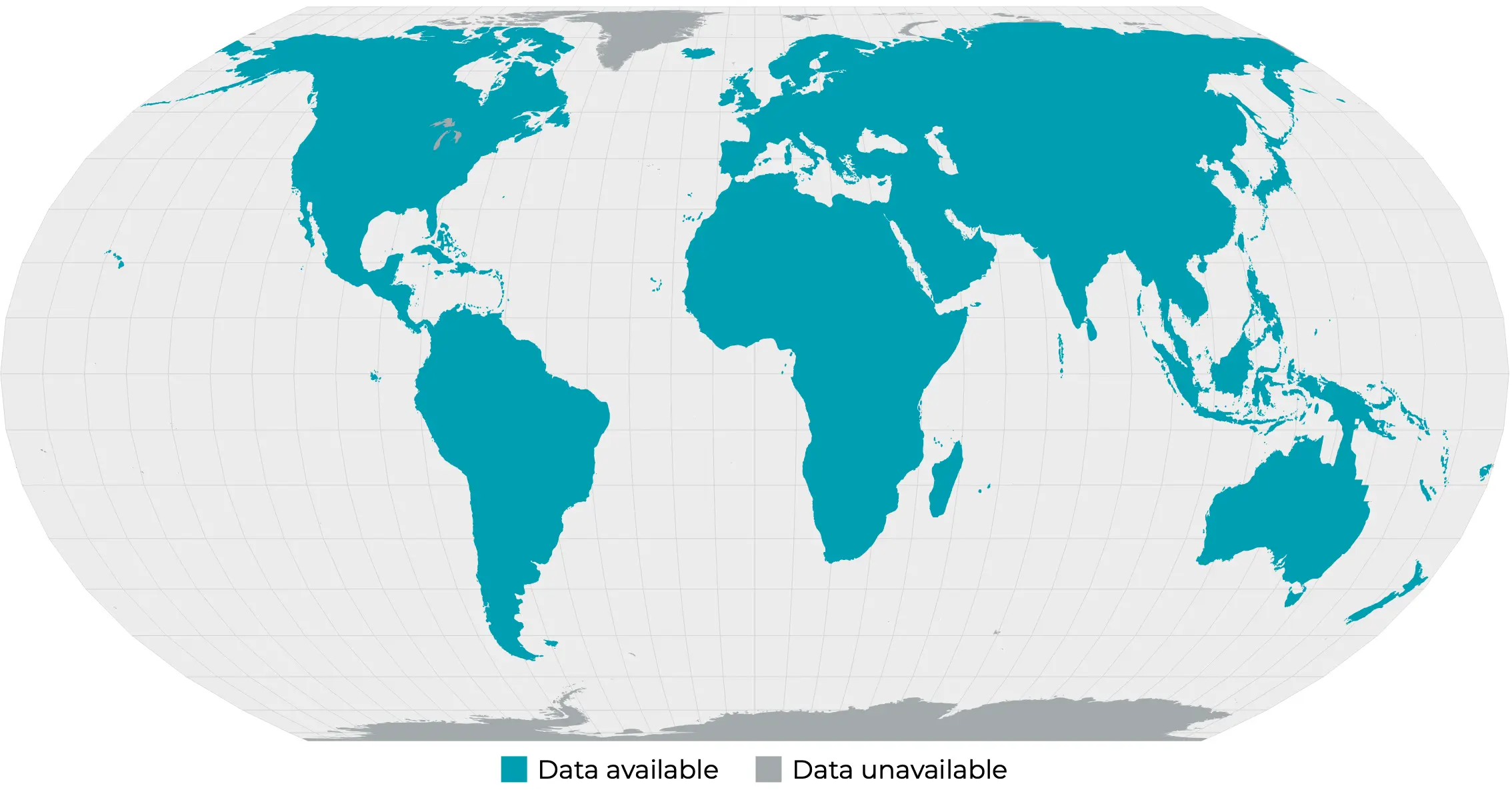
Figure 7. Data availability map for the forest carbon diligence product. Land above 75 North or below 60 South are excluded. Some small islands were excluded