# Planet Documentation > Generated LLMS index and full text for Planet documentation. - [Planet Documentation](https://docs.planet.com/index.md) ## data - [Data Catalog](https://docs.planet.com/data.md): Analytic Feeds - [Analytic Feeds](https://docs.planet.com/data/analytic-feeds.md) - [Aircraft Detection](https://docs.planet.com/data/analytic-feeds/aircraft-detection.md): Detect and monitor aircraft on airfields and tarmacs. - [Technical Specification](https://docs.planet.com/data/analytic-feeds/aircraft-detection/techspec.md): Key Product Features - [Road & Building Change Detection](https://docs.planet.com/data/analytic-feeds/road-building-change-detection.md): Detect changes in roads and buildings infrastructure. - [Technical Specification](https://docs.planet.com/data/analytic-feeds/road-building-change-detection/techspec.md): Key Product Features - [Vessel Detection](https://docs.planet.com/data/analytic-feeds/vessel-detection.md): Detect and monitor vessel over maritime areas. - [Technical Specification](https://docs.planet.com/data/analytic-feeds/vessel-detection/techspec.md): Planet’s Vessel Detection and Classification products leverage advanced machine learning and computer vision techniques to identify maritime activity over vast areas of interest. Derived from high-frequency PlanetScope imagery, this solution provides automated, oriented bounding box detections of vessels, enabling customers to monitor maritime domains, secure coastlines, and analyze economic activity with precision. - [Area Monitoring](https://docs.planet.com/data/area-monitoring.md): Sentinel Hub is a multi-spectral, temporal satellite imagery service for real-time processing of large remote sensing datasets. - [Applications](https://docs.planet.com/data/area-monitoring/applications.md): Applications - [Admin Application](https://docs.planet.com/data/area-monitoring/applications/admin-application.md): Admin Application - [Area Monitoring Application](https://docs.planet.com/data/area-monitoring/applications/area-monitoring-browser.md): Area Monitoring Application - [Expert Judgement Application](https://docs.planet.com/data/area-monitoring/applications/expert-judgement-application.md): Expert Judgement Application - [Geotagged Photo Application](https://docs.planet.com/data/area-monitoring/applications/geotagged-photo-application.md): Geotagged Photo Application - [Common](https://docs.planet.com/data/area-monitoring/common.md): Details of commonly used properties and objects - [Marker Service API](https://docs.planet.com/data/area-monitoring/marker-service-api.md): Documentation on the structure of the markers's data served through API - [Markers](https://docs.planet.com/data/area-monitoring/markers.md): Markers - [Bare-Soil Marker](https://docs.planet.com/data/area-monitoring/markers/bare-soil-marker.md): Bare-Soil Marker - [Bare-Soil Marker Examples](https://docs.planet.com/data/area-monitoring/markers/bare-soil-marker/examples.md): Bare-Soil Marker Examples - [Binary Land-Cover Marker](https://docs.planet.com/data/area-monitoring/markers/binary-land-cover-marker.md): Binary Land-Cover Marker - [Binary Land-Cover Marker Examples](https://docs.planet.com/data/area-monitoring/markers/binary-land-cover-marker/examples.md): Binary land-cover marker examples - [Crop and Land-Use Markers](https://docs.planet.com/data/area-monitoring/markers/crop-and-land-use-markers.md): Crop and Land-Use Markers - [Crop and Land-Use Marker Examples](https://docs.planet.com/data/area-monitoring/markers/crop-and-land-use-markers/examples.md): Crop and land-use marker examples - [Field Delineation](https://docs.planet.com/data/area-monitoring/markers/field-delineation.md): Field Delineation - [Greening and Harvest Marker](https://docs.planet.com/data/area-monitoring/markers/greening-harvest-marker.md): Greening and Harvest Marker - [Greening and Harvest Marker Examples](https://docs.planet.com/data/area-monitoring/markers/greening-harvest-marker/examples.md): Greening and Harvest Marker Examples - [Homogeneity Marker](https://docs.planet.com/data/area-monitoring/markers/homogeneity-marker.md): Homogeneity Marker - [Homogeneity Marker Examples](https://docs.planet.com/data/area-monitoring/markers/homogeneity-marker/examples.md): Homogeneity Marker Examples - [Mowing Marker](https://docs.planet.com/data/area-monitoring/markers/mowing-marker.md): Mowing Marker - [Mowing Marker Examples](https://docs.planet.com/data/area-monitoring/markers/mowing-marker/examples.md): Mowing Marker Examples - [Ploughing Marker](https://docs.planet.com/data/area-monitoring/markers/ploughing-marker.md): Ploughing Marker - [Similarity and Euclidian Distance Marker](https://docs.planet.com/data/area-monitoring/markers/similarity-and-euclidian-distance-marker.md): Similarity and Euclidian Distance Marker - [Similarity and Euclidian Distance Marker Examples](https://docs.planet.com/data/area-monitoring/markers/similarity-and-euclidian-distance-marker/examples.md): Similarity and Euclidian Distance Marker Examples - [References](https://docs.planet.com/data/area-monitoring/references.md): References - [Signal Processing](https://docs.planet.com/data/area-monitoring/signal-processing.md): Signal Processing - [Traffic Light System](https://docs.planet.com/data/area-monitoring/traffic-light-system.md): Traffic Light System - [Traffic Light System Examples](https://docs.planet.com/data/area-monitoring/traffic-light-system/examples.md): Traffic Light System Examples - [Videos](https://docs.planet.com/data/area-monitoring/videos.md): Videos - [Visualizations](https://docs.planet.com/data/area-monitoring/visualizations.md): Documentation for visualization of area monitoring results - [Communication](https://docs.planet.com/data/area-monitoring/visualizations/communication.md): Documentation for Communication React component - [Marker Scores](https://docs.planet.com/data/area-monitoring/visualizations/marker-scores.md): Documentation for Marker Scores React component - [Markers Summary](https://docs.planet.com/data/area-monitoring/visualizations/markers-summary.md): Documentation for Markers Summary React component - [Observation](https://docs.planet.com/data/area-monitoring/visualizations/observation.md): Documentation for Observation React component - [Photo Task Creator](https://docs.planet.com/data/area-monitoring/visualizations/photo-task-creator.md): Documentation for Photo Task Creator React component - [Pixel Mowing](https://docs.planet.com/data/area-monitoring/visualizations/pixel-mowing.md): Documentation for visualization of pixel mowing marker results - [Signal Marker Visualization](https://docs.planet.com/data/area-monitoring/visualizations/signal-marker-visualization.md): Documentation for Signal Marker Visualization React component - [Timelapse](https://docs.planet.com/data/area-monitoring/visualizations/timelapse.md): Documentation for Timelapse React component - [Planet Imagery](https://docs.planet.com/data/imagery.md) - [Analysis-Ready PlanetScope](https://docs.planet.com/data/imagery/arps.md): Information about Analysis-Ready PlanetScope - [Analysis-Ready PlanetScope Sandbox Data](https://docs.planet.com/data/imagery/arps/sandbox.md) - [Technical Specification v1.0](https://docs.planet.com/data/imagery/arps/techspec/v1-0-0.md): Publicly available flight data is incomplete, often omitting sensitive military movements, private flights, and activity in conflict zones. This leaves analysts with significant blind spots. The traditional alternative — manual analysis of satellite imagery — is slow, expensive, and impossible to scale across thousands of airfields. As a result, monitoring has been limited to a select number of locations with sporadic coverage, providing only isolated snapshots in time rather than a comprehensive view.
In a world of rapid geopolitical change, relying on incomplete data or slow, manual processes means missing critical indicators and failing to see the bigger picture of global movements.

### Automated, Global Monitoring From Space Planet Aircraft Detection transforms airfield monitoring from a tedious, manual task into an automated, scalable solution. By applying a sophisticated machine learning model to our global, near-daily PlanetScope® imagery, we provide **automated detections of aircraft at rest on airfields across the entire world.**
This represents the first-ever attempt at global detection of large aircraft on a near-daily basis from satellite imagery. Instead of sporadic checks on a few known airfields, you gain a persistent, foundational layer of intelligence over any airport or airstrip of interest. Our solution enables pattern-of-life analysis, allowing you to establish baseline activity, automatically detect anomalies, and receive alerts on significant changes — empowering analysts of all backgrounds to move faster and with greater confidence.
Planet's ability to systematically scan airfields around the globe unlocks new analytical capabilities for defense, intelligence, and commercial organizations.
### Defense and Intelligence Analysis For defense and intelligence agencies, understanding an adversary’s force posture and movements is paramount. Public flight data is often ineffective in sensitive or denied areas. Planet Analytic Feeds for Aircraft Detection provides a reliable, non-cooperative method for monitoring military airbases. * **Track fleet deployments:** Count aircraft at an airbase and see where they reappear, providing insight into strategic movements. * **Establish baselines and detect anomalies:** Automatically monitor airfields to establish normal patterns and receive alerts when unusual numbers or types of aircraft arrive or depart. * **Enhance situational awareness:** Provide objective, evidence-based intelligence on global military activity without relying on public reporting.
**Planet’s Unique Approach.** Our near-daily coverage of Earth's landmass means you are no longer restricted to monitoring a handful of known sites. You can monitor all of them, ensuring you never miss a critical development.
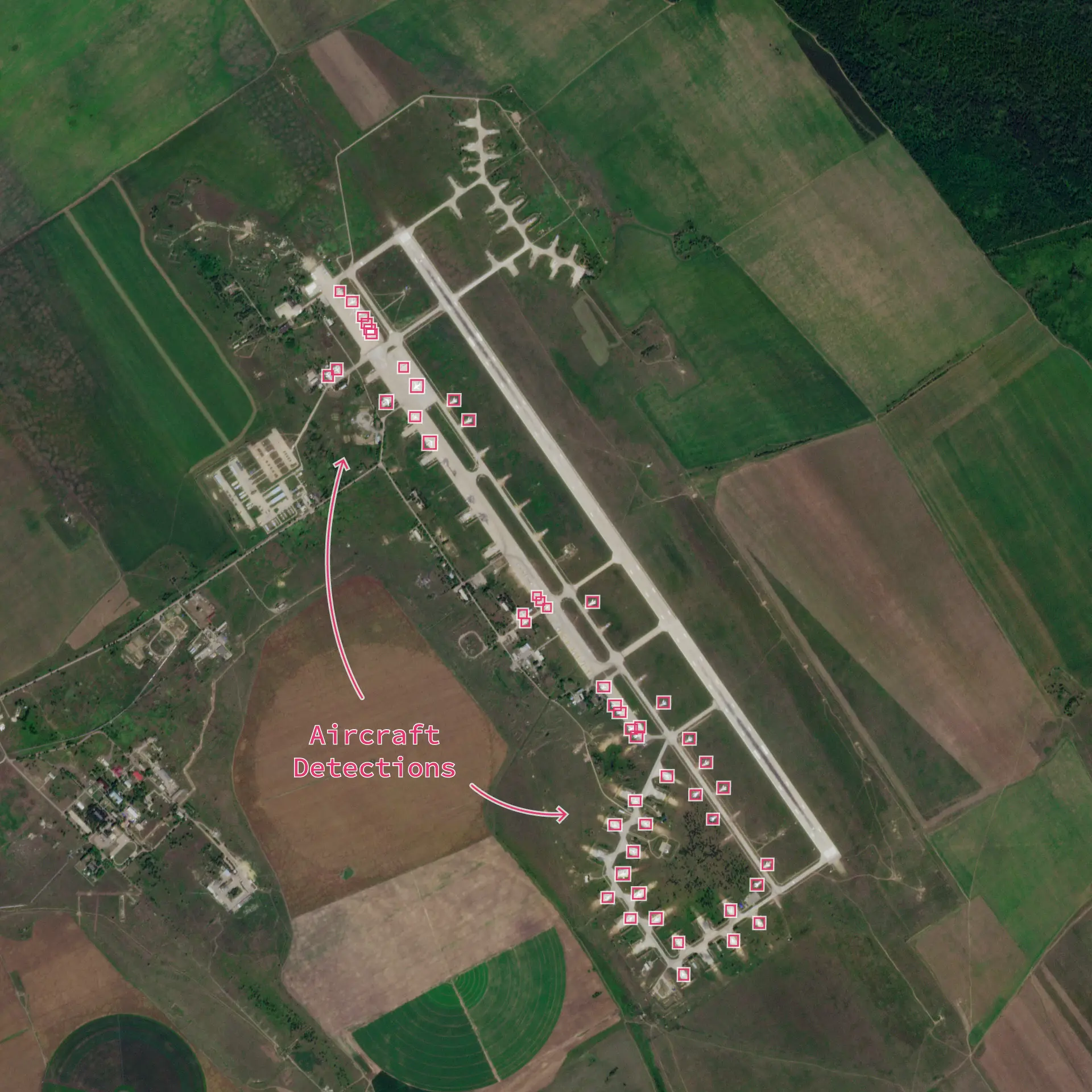
![Example of aircraft detection](/data/analytic-feeds/aircraft-detection/aircraft_belya.webp)
### Economic Intelligence and Trend Analysis The movement of commercial and cargo aircraft is a useful proxy for economic activity. Analysts can leverage our feed to gain a competitive edge and validate other economic indicators. * **Predict economic trends:** Monitor the volume of cargo and executive jets at key airports to gauge supply chain activity and corporate travel. * **Assess event impact:** Quantify the influx of air traffic for major global events like sporting championships or political summits to measure their economic impact. * **Improve market models:** Integrate a novel, global dataset into economic models for more accurate forecasting.
**Planet’s Unique Approach.** The sheer scale of our automated detection provides a macro-level view of economic activity that is impossible to replicate with other sources, giving commercial analysts an unprecedented data source. ## API Information | API | Available | Notes | | ----------------- | --------- | --------------------------------------------------------------------------------------------------------------------------- | | Data API | ✅ | Customers can use the Data API to query imagery associated with an aircraft detection analytic subscription | | Orders API | ✅ | Customers can use the Orders API to order imagery associated with an aircraft detection analytic subscription | | Subscriptions API | ✅ | Customers can use the Subscriptions API to subscribe to imagery associated with an aircraft detection analytic subscription | | Analytics API | ✅ | The Analytics API is used to query aircraft detection results | | Basemaps API | ❌ | | --- Copy for LLM[View as Markdown](https://docs.planet.com/data/analytic-feeds/aircraft-detection/techspec/) # Technical Specification ### Key Product Features With Planet Analytic Feeds for Aircraft Detection, you receive an end-to-end solution designed for immediate integration and analysis. * **Full imagery access.** You receive full access to the underlying PlanetScope imagery within your area of interest, including the ability to stream image tiles or download GeoTIFFs for visual verification, detailed analysis, and reporting. Our imagery provides clear, 3.7 m resolution evidence. * **Automated aircraft detections.** Detections for aircraft ≥ 20 m in length or wingspan are delivered as GeoJSON feature collections via our Analytics API or visualized in our Feed Viewer. This data is ready for immediate integration into your existing GIS platforms and analytical workflows. ### Methodology Our model is built on a foundation of cutting-edge machine learning techniques and a unique approach to data labeling, ensuring reliable performance at a global scale. We utilize a deep learning object detection model optimized to run efficiently on our medium-resolution PlanetScope imagery. This allows us to analyze thousands of airfields daily to identify aircraft at rest on tarmacs and runways.
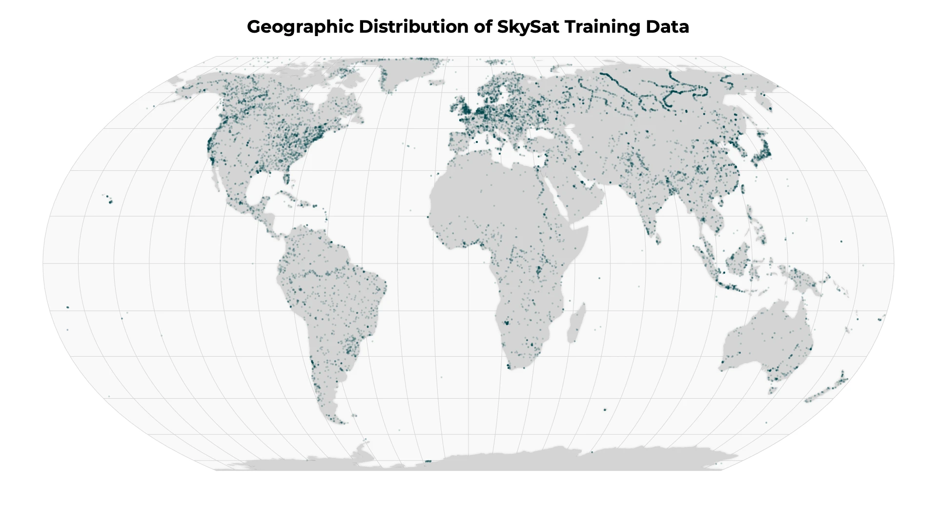
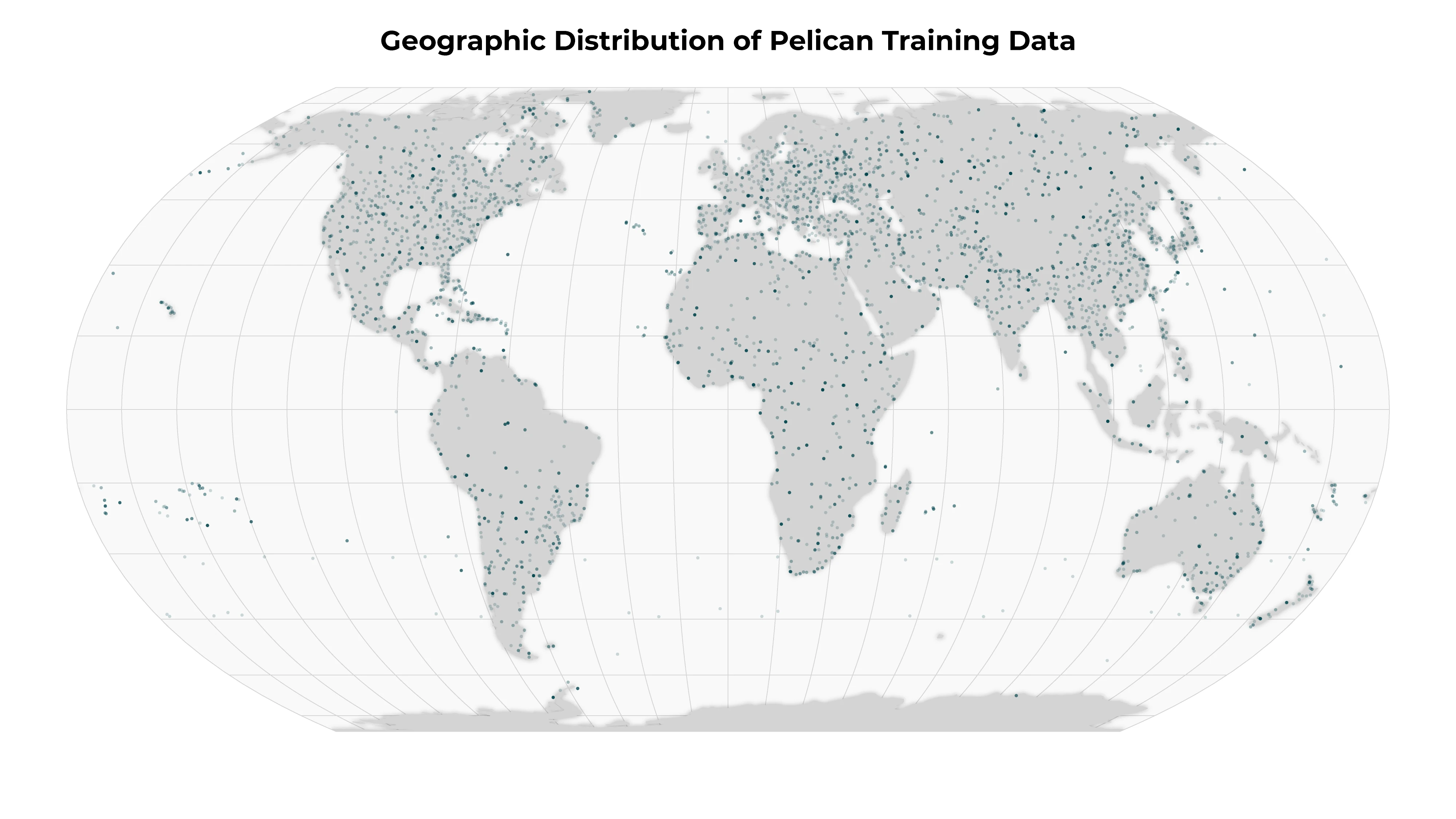
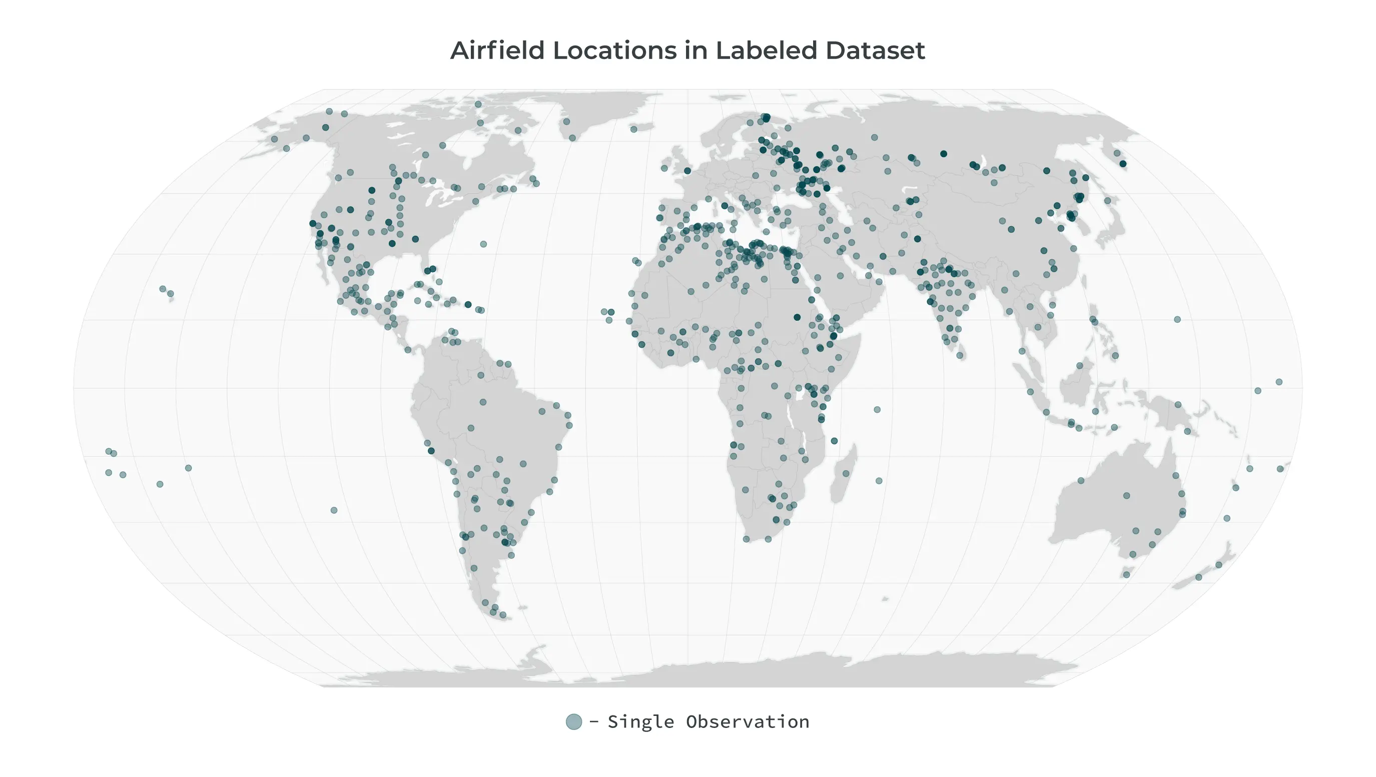
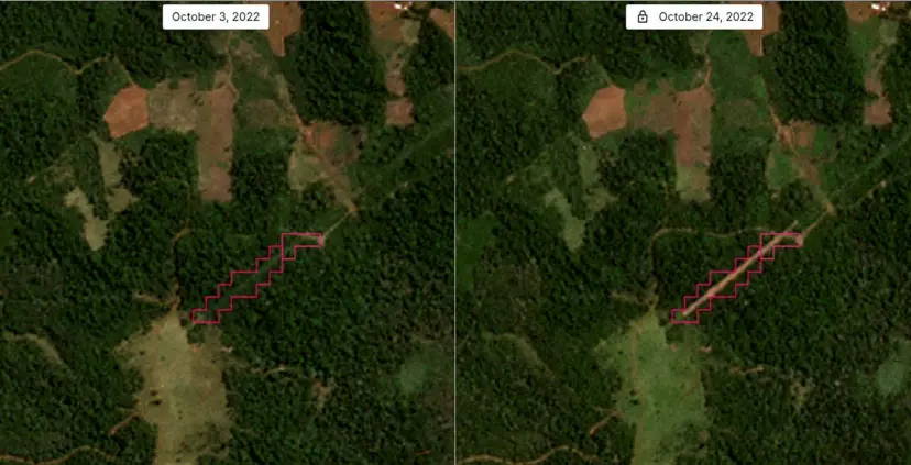
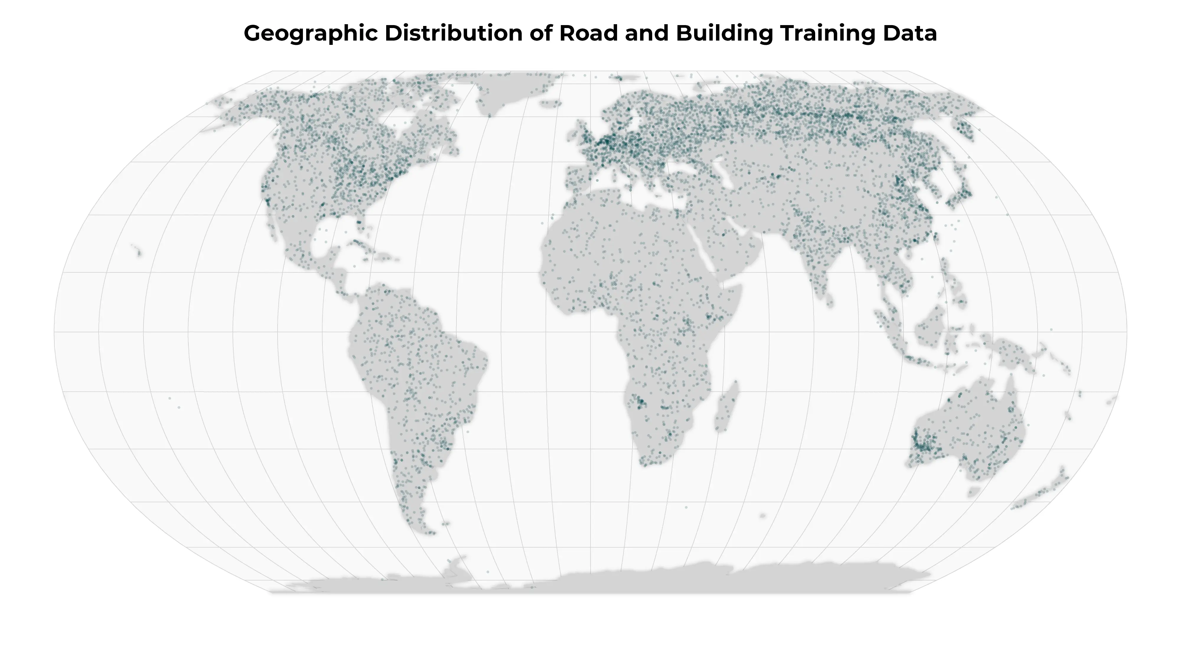
#### Unique Training Data Approach To achieve high accuracy, we developed an innovative labeling process. We use high-resolution SkySat® imagery captured within three minutes of a PlanetScope image. Our expert labelers identify aircraft in the crisp SkySat imagery, and those high-fidelity labels are then transferred to the corresponding PlanetScope scene. This unique multi-resolution approach ensures our model is trained on the most accurate ground truth data possible. ![Example of aircraft detection](/data/analytic-feeds/aircraft-detection/aircraft_label_gif.webp) #### Robust Training Data The model was trained on a curated dataset of over 15,000 labels derived from concurrent pairs of SkySat and PlanetScope images. This dataset has a broad geographic and temporal distribution, covering hundreds of airfields worldwide across multiple years and all seasons. This diversity ensures the model is robust and performs reliably in a wide variety of real-world conditions. It is continually updated and expanded to reduce model drift and address issues as they arise. ![Aircraft Detection Model Training Dataset](/data/analytic-feeds/aircraft-detection/training_data_aircraft.webp) #### Reliable Performance The model is rigorously tested against a globally distributed test set, achieving a high level of accuracy for detecting aircraft ≥20 meters. * **Precision: 0.87** - This measures the accuracy of our detections. A high precision score means that when we identify an aircraft, it is highly likely to be a true aircraft, minimizing false alarms. * **Recall: 0.78** - This measures the completeness of our detections. A high recall score means we successfully identify a high percentage of the actual aircraft vessels present in the imagery. * **F1-Score: 0.82** - This provides a single, balanced measure of the model's overall accuracy by combining both precision and recall. ### Delivery Mechanisms Results are available via the Analytics API and Feed Viewer. For more details please see: * **[Analytics API](https://docs.planet.com/develop/apis/analytics.md)** * **[Feed Viewer](https://docs.planet.com/platform/get-started/analyze-data/analytic-feeds-viewer.md)** ### Full Metadata Reference #### Feature-level Fields | Property | Format | Example | Definition | | -------- | --------------------- | ------------------------------------------------- | -------------------------------------------------------------------------------------------- | | created | ISO 8601 DateTime | "2026-02-03T19:02:45.270966Z" | The timestamp when the feature was created in the system | | geometry | GeoJSON Geometry | `{"type": "Polygon", "coordinates": [...]}` | The geographic polygon defining the location of the detected change | | id | UUID | "17f21835-93c4-4664-b2ef-c2f57f5809a5" | The unique identifier for the feature | | links | Array of Link Objects | `[{"href": "...", "rel": "self", "type": "..."}]` | Array of related resources including visual tiles, quads, process info, and observation data | | type | String | "Feature" | The GeoJSON feature type | #### Properties | Property | Format | Example | Definition | | ----------------------------- | ----------------- | ------------------------------------------------------------------------------------------------------------------------------------------------------------------------------------------------------------------------- | ------------------------------------------------------------------------------------------------------------ | | bbox\_area\_m2 | Float | 1292.76 | The area of the detected aircraft's bounding box in square meters | | bbox\_diagonal\_m | Float | 51.09171557111779 | The diagonal length of the aircraft bounding box in meters | | bbox\_length\_m | Float | 38.55 | The estimated length of the aircraft in meters | | bbox\_width\_m | Float | 33.53 | The estimated width of the aircraft in meters | | category | String | "aircraft" | The category of the detected object | | model\_id | String | "toothless\_aircraft" | The identifier of the detection model used | | model\_version | String | "toothless-aircraft-ps-v1.2.0" | The version of the detection model used | | object\_class\_label | String | "aircraft" | The classification label assigned to the detected object | | observed | ISO 8601 DateTime | "2026-02-09T08:09:38.541005Z" | The timestamp when the aircraft was observed | | score | Float | 0.805 | The model's confidence in the detection accuracy (0-1 scale, where higher values indicate greater certainty) | | source\_asset\_type | String | "ortho\_visual" | The type of asset used for detection | | source\_cloud\_cover | Float | 0.83 | The cloud cover percentage in the source imagery (0-1 scale) | | source\_extent | WKT Polygon | "POLYGON ((51.1546410707396575 35.7877539840997514, 51.1144425763138770 35.6347767140370664, 51.4287071306998484 35.5791382492902173, 51.4695444327112881 35.7324398323834131, 51.1546410707396575 35.7877539840997514))" | The geographic extent of the source imagery as a polygon | | source\_image\_mean\_gsd | Float | 3.3 | The mean ground sample distance of the source imagery in meters | | source\_item\_id | String | "20260209\_080938\_54\_24fd" | The unique identifier of the source imagery item | | source\_item\_type | String | "PSScene" | The type of source imagery item | | source\_quality\_category | String | "standard" | The quality category of the source imagery | | source\_sun\_azimuth\_angle | Float | 167.5 | The azimuth angle of the sun in the source imagery in degrees | | source\_sun\_elevation\_angle | Float | 38.8 | The elevation angle of the sun in the source imagery in degrees | In an increasingly dynamic world, waiting for reports is no longer an option. Planet Aircraft Detection provides the persistent, global awareness needed to understand airfield activity as it happens. Move beyond manual analysis and incomplete data to a new paradigm of automated insight. See the full picture, detect critical changes first, and act with the speed and confidence that only Planet can deliver. --- Copy for LLM[View as Markdown](https://docs.planet.com/data/analytic-feeds/road-building-change-detection/) # Road & Building Change Detection ![Header Thumbnail](/data/analytic-feeds/road-building-change-detection/thumbnail.webp) Keeping up to date with human development is a daunting task, especially when scanning across enormous country-wide areas. Government agencies throughout the world are challenged to ensure protected areas remain untouched and that development only takes place when it is properly permitted. But even with the growth of satellite observations, identifying new activity in massive archives of data is costly and time-intensive. Planet’s Road & Building Change Detection products point users to where development is taking place across country-wide areas on a weekly basis, helping them understand exactly how and where the places they care most about are evolving. Drawing on Planet’s daily scan of the Earth, analysts can look at activities as they unfold without the burden of sifting through huge volumes of imagery. ### Permit Enforcement ![Example of road change detection](/data/analytic-feeds/road-building-change-detection/nmslo.webp) New road construction in southeastern New Mexico detected in the Analytics Feed Viewer. The New Mexico State Land Office compares Road Change Detections with permit applications to determine if development has taken place prior to permit approval. They were able to generate an estimated $1M in revenue from permit violations discovered using Road Change Detection. ### Monitoring Protected Areas ![Example of road change detection](/data/analytic-feeds/road-building-change-detection/brazil.webp) New road construction in the Misiones Province of eastern Argentina detected in the Analytics Feed Viewer. Policia Federal of Brazil leverages Road & Building Change Detections to draw their attention to where and when development is taking place within protected forested areas. ## API Information | API | Available | Notes | | ----------------- | --------- | ------------------------------------------------------------------------------------------------------------------------------------------------------------------------------------------------------------------------------ | | Data API | ❌ | Road & Building Change Detection runs on a weekly or monthly cadence, providing weekly or monthly visual mosaics alongside change detections. The Data API supports querying scene information only. | | Orders API | ✅ | Road & Building Change Detection runs on a weekly or monthly cadence, providing weekly or monthly visual mosaics alongside change detections. The Orders API supports ordering mosaic quads. | | Subscriptions API | ❌ | Road & Building Change Detection runs on a weekly or monthly cadence, providing weekly or monthly visual mosaics alongside change detections. The Subscriptions API does not currently support subscriptions for mosaic quads. | | Analytics API | ✅ | The Analytics API is used to query Road & Building Change Detection results. | | Basemaps API | ✅ | Road & Building Change Detection runs on a weekly or monthly cadence, providing weekly or monthly visual mosaics alongside change detections. The Basemaps API supports querying and delivering mosaic quads. | --- Copy for LLM[View as Markdown](https://docs.planet.com/data/analytic-feeds/road-building-change-detection/techspec/) # Technical Specification ### Key Product Features With Planet Analytic Feeds for Road and Building Change Detection, you receive an end-to-end solution designed for immediate integration and analysis. | Product | Cadence | Includes | Format | Delivery | Web Application | | ------------------------- | ----------------- | ------------- | -------------- | ---------------------------------------------------------------------------------------------------------------------------------------------------------------------------------------------------- | ------------------------------------------------------------------------------------------------- | | Road Detection | Weekly or Monthly | Visual Mosaic | Raster Geotiff | [Analytics API](https://docs.planet.com/develop/apis/analytics.md), [Basemaps API](https://docs.planet.com/develop/apis/basemaps.md), [Tile Services](https://docs.planet.com/develop/apis/tiles.md) | [Feed Viewer](https://docs.planet.com/platform/get-started/analyze-data/analytic-feeds-viewer.md) | | Building Detection | Weekly or Monthly | Visual Mosaic | Raster Geotiff | [Analytics API](https://docs.planet.com/develop/apis/analytics.md), [Basemaps API](https://docs.planet.com/develop/apis/basemaps.md), [Tile Services](https://docs.planet.com/develop/apis/tiles.md) | [Feed Viewer](https://docs.planet.com/platform/get-started/analyze-data/analytic-feeds-viewer.md) | | Road Change Detection | Weekly or Monthly | Visual Mosaic | Vector Geojson | [Analytics API](https://docs.planet.com/develop/apis/analytics.md) | [Feed Viewer](https://docs.planet.com/platform/get-started/analyze-data/analytic-feeds-viewer.md) | | Building Change Detection | Weekly or Monthly | Visual Mosaic | Vector Geojson | [Analytics API](https://docs.planet.com/develop/apis/analytics.md) | [Feed Viewer](https://docs.planet.com/platform/get-started/analyze-data/analytic-feeds-viewer.md) | ### Methodology Planet’s Road & Building Change Detection takes a multiple step approach. At a high level, we run a semantic segmentation model on all the PlanetScope imagery published in a given area for a given week or month to assign a probability value (0-255) that the pixel represents a road, building or neither object. The segmentation model results are aggregated together into a weekly or monthly layer and this process is repeated through time, generating a time-series of pixel values. Using the historical results, we run a predictive time series model to estimate what a given pixel’s value for a given time point should be compared to the actual observed value. When these values differ significantly, we create a change detection polygon indicating road or building development. ### Segmentation Model Planet’s Road & Building segmentation model is a modified UNET, a deep learning supervised segmentation model, that runs on 4-band (RGBNir) Surface Reflectance assets. It was trained on \~10 thousand Planetscope images paired with labels pulled from Microsoft’s open [roads](https://github.com/microsoft/RoadDetections) and [buildings](https://github.com/microsoft/GlobalMLBuildingFootprints) datasets to mark each pixel into one of 3 classes: Road, Building, or other. [](/data/analytic-feeds/road-building-change-detection/rb1.mp4) Planet's Road & Building segmentation model assigns a probability value (0-255) that a pixel represents a road, building, or neither object. Planet leveraged 80% of the dataset to train the segmentation model, holding out 20% of the labeled dataset for validation to measure the model's performance. By comparing the model's results over this 20% holdout dataset, we are able to calculate the following precision, recall, and F1 measurements: ![Training Dataset Distribution](/data/analytic-feeds/road-building-change-detection/rbdataset.webp) Global locations of the training data used to train the Road and Building detection segmentation model. | Class | F1 | Precision | Recall | | ---------- | ---- | --------- | ------ | | Road | 0.72 | 0.77 | 0.68 | | Building | 0.81 | 0.81 | 0.81 | | Background | 0.99 | 0.99 | 0.99 | ### Result Aggregation Planet publishes imagery just about everywhere, just about every day. While the model was trained and runs on individual images, we are able to generate even better results when we take advantage of the data density PlanetScope provides. For a given area, we run the segmentation model on all of the published PlanetScope data for a given week and then aggregate those results into a single weekly result. This process removes any noisy detections caused by atmospheric interference, provides the greatest coverage and generally ensures the best possible representation of roads and buildings for the location. [](/data/analytic-feeds/road-building-change-detection/rb2.mp4) Daily results are aggregated into weekly or monthly layers, providing a consistent time series to analyze. ### Change Detection With the segmentation output aggregated to weekly results, we generate time series data that tracks a pixel’s segmentation value through time. Leveraging this information, we are able to run a predictive model that establishes an expectation of what the pixel value should be for any given time point. We then compare this predicted value to the observed value to calculate the number of standard deviations (or “z-score”) between what is expected and the observed value. [](/data/analytic-feeds/road-building-change-detection/rb3.mp4) Time series data is analyzed to spot areas of development where pixel values have shifted significantly. By evaluating this z-score through time, we found that z-scores greater than 10.5 indicated a high likelihood of real change taking place and results under this threshold were predominantly false positives. Because of this, we filter out any detections with a z-score under 10.5. We map the z-score to a “confidence score” between 0.5 and 1.0 that is surfaced in the metadata of the change detection. The higher the z-score, the closer the confidence score gets to 100%. Generally detections will have confidence scores between 50% and 75%. Our change detection polygons are mapped to a standard 8x8 pixel gridcell, highlighting the area where the change took place. Measuring the change detection model’s recall is difficult, since there is not a standard ground truth dataset that we can measure against. Any dataset we create would be powered by the change detection model itself, and it is hardly reasonable to measure it against itself. Still, we have been able to measure its precision. Manually validating hundreds of change events sampled across more than 100 regions, we found the model to have a precision of 0.94. While we have done our best to be exhaustive, we strongly suggest running a trial over your area to determine how well it performs to confirm it will work for your use case. ### Delivery Mechanisms Results are available via the Analytics API and Feed Viewer. For more details please see: * **[Analytics API](https://docs.planet.com/develop/apis/analytics.md)** * **[Feed Viewer](https://docs.planet.com/platform/get-started/analyze-data/analytic-feeds-viewer.md)** ### Full Metadata Reference #### Feature-level Fields | Property | Format | Example | Definition | | -------- | --------------------- | ------------------------------------------------- | -------------------------------------------------------------------------------------------- | | created | ISO 8601 DateTime | "2026-02-03T19:02:45.270966Z" | The timestamp when the feature was created in the system | | geometry | GeoJSON Geometry | `{"type": "Polygon", "coordinates": [...]}` | The geographic polygon defining the location of the detected change | | id | UUID | "17f21835-93c4-4664-b2ef-c2f57f5809a5" | The unique identifier for the feature | | links | Array of Link Objects | `[{"href": "...", "rel": "self", "type": "..."}]` | Array of related resources including visual tiles, quads, process info, and observation data | | type | String | "Feature" | The GeoJSON feature type | #### Properties | Property | Format | Example | Definition | | -------------------- | ----------------- | ------------------------------------------------------------------ | ---------------------------------------------------------------------------------------------------------------- | | change\_direction | String | "positive" | The direction of change detected (positive indicates new development) | | class\_label | String | "road" | The classification label for the type of infrastructure detected (road or building) | | date | ISO 8601 DateTime | "2026-02-02T00:00:00Z" | The end date of the observation period when the change was detected | | model\_version | String | "production" | The version of the model used for detection | | object\_area\_m2 | Float | 461.042850935856 | The area of the detected change in square meters | | object\_class\_label | String | "positive" | The classification label indicating the type of change | | observed | ISO 8601 DateTime | "2026-01-26T00:00:00Z" | The start date of the observation period | | score | Float | 0.5937995365687779 | The model's confidence in the detection accuracy (0.5-1.0 scale, where higher values indicate greater certainty) | | source\_mosaic\_name | String | "rnb\_weekly\_v2\_2026\_01\_26\_2026\_02\_02" | The name of the source mosaic used for detection | | source\_quad\_id | String | "1140-1295" | The identifier of the source quad tile | | visual\_mosaic\_name | String | "ps\_weekly\_visual\_subscription\_2026-01-26\_2026-02-02\_mosaic" | The name of the visual mosaic for imagery display | | visual\_quad\_id | String | "1140-1295" | The identifier of the visual quad tile | With Planet Road & Building Change Detection, you gain a robust, persistent, and reliable view of development over the areas you care most about. --- Copy for LLM[View as Markdown](https://docs.planet.com/data/analytic-feeds/vessel-detection/) # Vessel Detection ![Header Thumbnail](/data/analytic-feeds/vessel-detection/thumbnail.webp) Vessel Detection provides automated identification and monitoring of maritime vessels, enabling tracking of shipping activities, maritime surveillance, and ocean management. ## Seeing Beyond the Horizon The global maritime domain is the lifeblood of our world. It accounts for approximately 90% of international trade, serves as a primary food source for billions of people, and is crucial for global energy production. However, monitoring this vast and complex environment is an immense challenge. With over 100,000 ships at sea at any given time, traditional surveillance methods struggle to keep up.
Governments, maritime agencies, and commercial stakeholders have long relied on cooperative tracking systems, such as the automatic identification system (AIS) and radio frequency (RF) signals. While useful, these systems have a critical flaw: they rely on vessels choosing to broadcast their location.
Nefarious actors, from potentially illicit fishing fleets to smugglers and hostile military vessels, can simply turn off their transponders, becoming dark ships that vanish from conventional monitoring systems. Dark ships leave critical gaps in situational awareness, making it nearly impossible to: * Detect potentially illegal activity in sovereign waters * Monitor strategic chokepoints for security threats * Effectively combat illicit fishing and activities that impact the environment * Efficiently deploy expensive patrol aircraft and ships ### Persistent, Non-Cooperative Monitoring From Space Planet addresses this challenge through our automated Vessel Detection product, which provides a foundational layer of truth for Maritime Domain Awareness (MDA). We leverage the unprecedented power of our PlanetScope® constellation — the world's largest fleet of Earth-imaging satellites — to deliver ongoing automated vessel detection over vast ocean areas, on a near-daily basis.
Unlike AIS, satellite image-derived vessel monitoring is non-cooperative. It does not matter if a vessel is broadcasting its location or not. If it is on the surface, we can see it. This capability transforms MDA from a reactive search to a proactive, persistent monitoring mission, enabling users to see the complete picture of activity at sea and focus their resources where they matter most.
Planet's unique ability to scan enormous areas of the ocean on a near-daily basis unlocks critical new capabilities for a wide range of use cases. ### National Security and Border Protection Navies, coast guards, and border agencies face the challenge of monitoring vast maritime territories, including exclusive economic zones (EEZs). Planet Vessel Detection delivers automated surveillance that spots dark ships and other threats, giving agencies the power to:
* **Detect and track vessels of interest** operating under emissions control (EMCON). * **Prioritize and cue high-value assets,** such as patrol aircraft and ships, directly to suspicious activity, thereby maximizing their effectiveness and reducing operational costs. * **Establish a pattern-of-life understanding** in high-interest areas, making it easier to spot anomalies that signal potential threats.
**Planet’s Unique Approach.** No other commercial provider offers near-daily electro-optical coverage at the scale required for meaningful national security monitoring. Our ability to scan over 10 million km² provides the tip-off that other systems miss. ### Illegal, Unreported and Unregulated (IUU) Fishing IUU fishing is a multi-billion-dollar illicit industry that threatens global food security and marine ecosystems. These operators frequently go dark to avoid detection while engaging in illegal activities like fishing in protected areas or conducting illegal ship-to-ship transfers.
* PlanetScope near-daily imagery and automated detections can pinpoint vessels operating in marine protected areas or regions where fishing is prohibited. * Our revisit rate allows analysts to identify potential transshipment events at sea, a key indicator of IUU fishing, by detecting vessels loitering in close proximity.
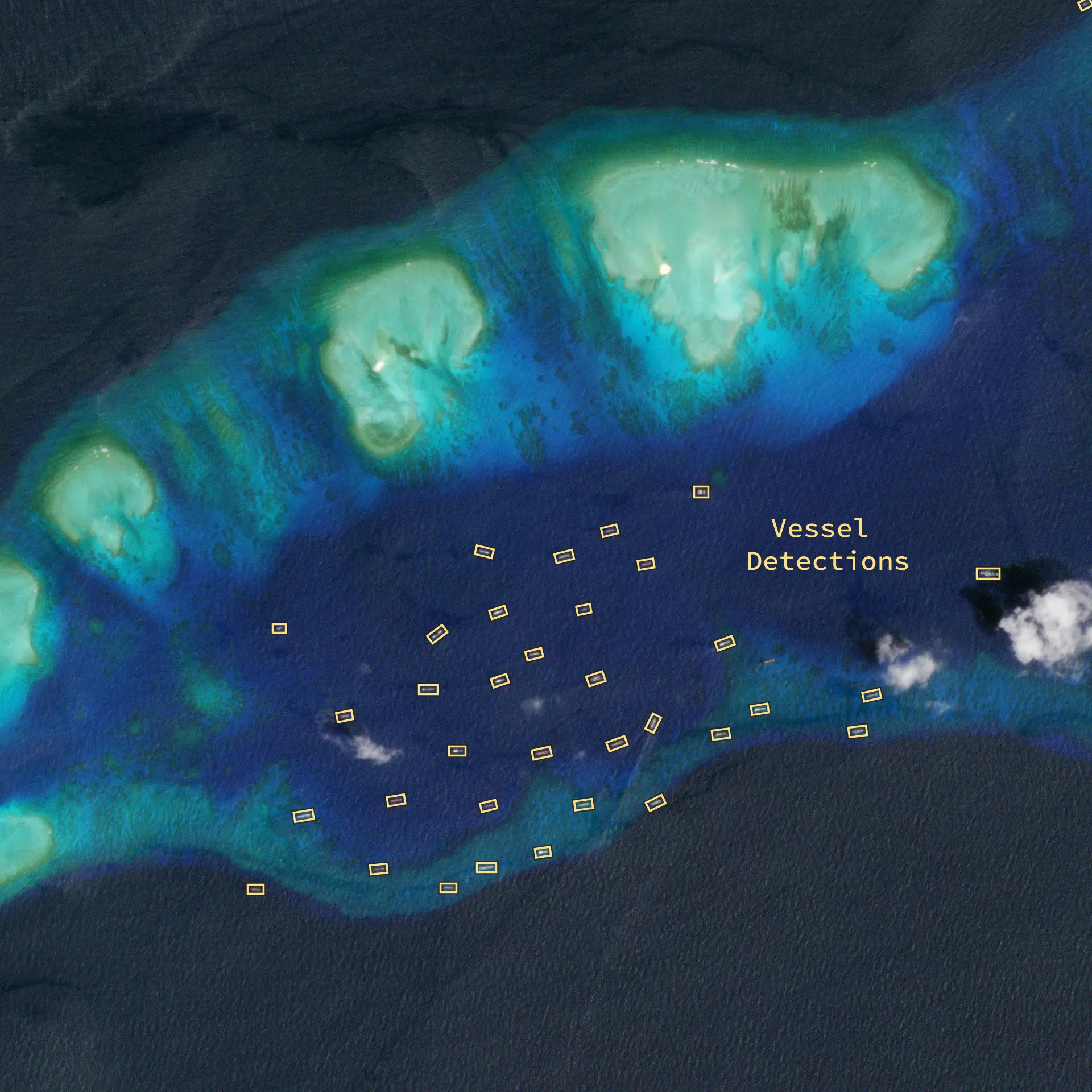
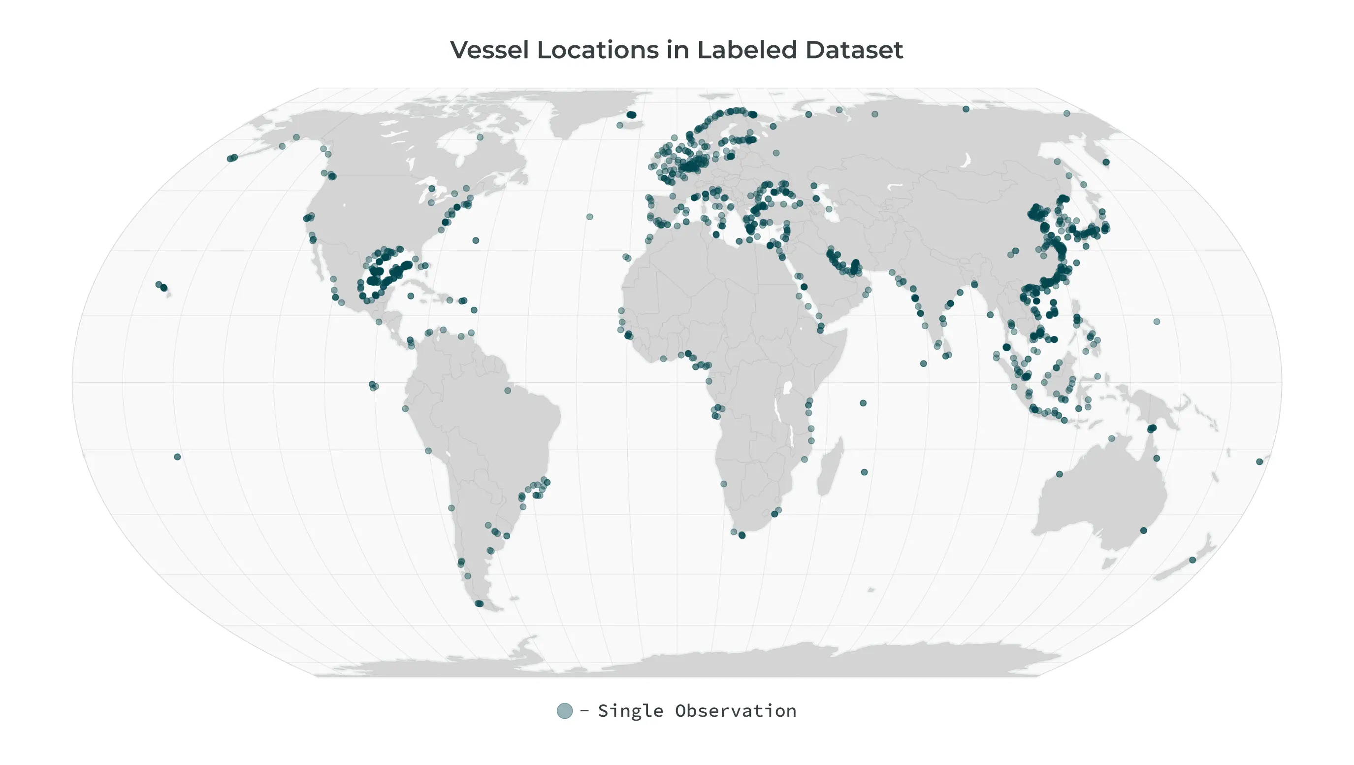
**Planet’s Unique Approach.** The PlanetScope constellation's near-daily revisit and broad area coverage are ideal for the persistent monitoring required to catch fleeting illegal fishing activities in remote ocean regions far from effective patrol routes. ## API Information | API | Available | Notes | | ----------------- | --------- | ------------------------------------------------------------------------------------------------------------------------------ | | Data API | ✅ | Customers can use the Data API to query imagery associated with a standard or enhanced vessel detection bundle | | Orders API | ✅ | Customers can use the Orders API to order imagery associated with a standard or enhanced vessel detection bundle | | Subscriptions API | ✅ | Customers can use the Subscriptions API to subscribe to imagery associated with a standard or enhanced vessel detection bundle | | Analytics API | ✅ | The Analytics API is used to query vessel detection results | | Basemaps API | ❌ | | --- Copy for LLM[View as Markdown](https://docs.planet.com/data/analytic-feeds/vessel-detection/techspec/) # Technical Specification Planet’s Vessel Detection and Classification products leverage advanced machine learning and computer vision techniques to identify maritime activity over vast areas of interest. Derived from high-frequency PlanetScope imagery, this solution provides automated, oriented bounding box detections of vessels, enabling customers to monitor maritime domains, secure coastlines, and analyze economic activity with precision. Planet supports three Vessel Detection offerings: * **Standard Vessel Detection:** Only provides geojson feature collections containing polygons indicating the location and time vessels were detected along with associated metadata (for example, estimated length/width/heading, confidence score and other relevant information). This is a good fit for users with existing access to maritime data/imagery. * **Standard Vessel Detection with Open Water Monitoring:** Includes everything for Standard Vessel Detection but also includes open water imagery over the area of interest. * **Enhanced Vessel Detection with Open Water Monitoring:** Additional metadata is included for vessel classification and bunkering status | | Standard Vessel Detection | Standard Vessel Detection with Open Water Monitoring | Enhanced Vessel Detection with Open Water Monitoring | | ----------------------------------------------- | ------------------------- | ---------------------------------------------------- | ---------------------------------------------------- | | Geojson Feature Collection of Vessel Detections | ✅ | ✅ | ✅ | | Estimated Width, Length, Heading | ✅ | ✅ | ✅ | | Confidence Score | ✅ | ✅ | ✅ | | Imagery | ❌ | ✅ | ✅ | | Vessel Classification | ❌ | ❌ | ✅ | | Bunkered status | ❌ | ❌ | ✅ | ### Methodology Our vessel detection model provides reliable, high-quality results that you can trust to drive critical decisions. The process uses a sophisticated deep learning approach. #### Validated Approach * **Segmentation:** The model first performs a segmentation step on the PlanetScope imagery. It analyzes the image pixel by pixel to create a probability mask that highlights all areas likely to contain a vessel. * **Polygonization and feature extraction:** The model then processes this mask to generate a precise, object-oriented bounding box around each probable vessel. During this step, it calculates key metadata for each detection, including the confidence score, estimated length, and heading. This two-step process is highly effective at identifying vessels longer than 25 m while minimizing false positives from other features on the ocean's surface. * **Classification and Bunkering:** For Enhanced Vessel Detection, we apply a secondary classification step that adds a predicted class property to the result, including Tanker, Cargo, and Military classes. We also add a status indicating if the vessel is closely bunkered with another ship to highlight potential ship-to-ship transfers. #### Robust Training Data A model is only as good as the data it is trained on. Planet Vessel Detection is trained on a massive, hand-labeled training dataset curated from our extensive imagery archive. This dataset features a broad geographic and temporal distribution, encompassing thousands of images from different oceans, seasons, and times of day. This diversity ensures the model is robust and performs reliably across a wide variety of real-world conditions, including different sea states, atmospheric haze, sun angles, and vessel types. It is continually updated and expanded to reduce model drift and address issues as they arise. ![Example of vessel detection](/data/analytic-feeds/vessel-detection/vessel_dataset.webp) #### Reliable Performance Our model is rigorously tested to ensure it meets the demanding needs of our users. Planet leveraged 80% of the above dataset to train the segmentation model, holding out 20% of the labeled dataset for validation to measure the model's performance. By comparing the model's results over this 20% holdout dataset, we can calculate the following precision, recall, and F1 measurements specifically over open water areas for vessels greater than 25 m in length. * **Precision: 0.87** - This measures the accuracy of our detections. A high precision score means that when we identify a vessel, it is highly likely to be an actual vessel, minimizing false alarms. * **Recall: 0.85** - This measures the completeness of our detections. A high recall score means we successfully identify a high percentage of the actual vessels present in the imagery. * **F1-Score: 0.86** - This provides a single, balanced measure of the model's overall accuracy by combining both Precision and Recall.
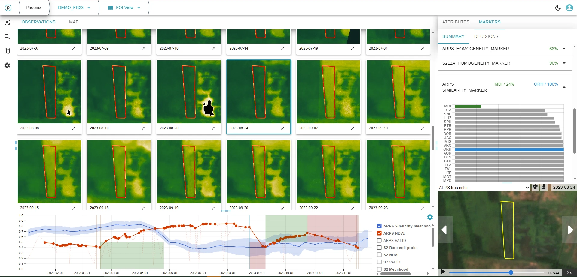
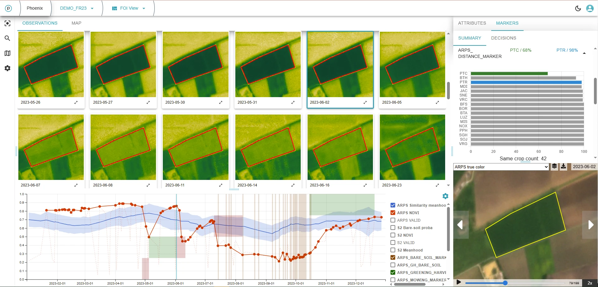
### Delivery Mechanisms Results are available via the Analytics API and Feed Viewer. For more details please see: * **[Analytics API](https://docs.planet.com/develop/apis/analytics.md)** * **[Feed Viewer](https://docs.planet.com/platform/get-started/analyze-data/analytic-feeds-viewer.md)** ### Full Metadata Reference #### Feature-level Fields | Property | Format | Example | Definition | | -------- | --------------------- | ------------------------------------------------- | -------------------------------------------------------------------------------------------- | | created | ISO 8601 DateTime | "2026-02-03T19:02:45.270966Z" | The timestamp when the feature was created in the system | | geometry | GeoJSON Geometry | `{"type": "Polygon", "coordinates": [...]}` | The geographic polygon defining the location of the detected change | | id | UUID | "17f21835-93c4-4664-b2ef-c2f57f5809a5" | The unique identifier for the feature | | links | Array of Link Objects | `[{"href": "...", "rel": "self", "type": "..."}]` | Array of related resources including visual tiles, quads, process info, and observation data | | type | String | "Feature" | The GeoJSON feature type | #### Properties | Property | Format | Example | Definition | | ----------------------------- | ----------------- | ------------------------------------------------------------------------------------------------------------------------------------------------------------------------------------------------------------------------- | --------------------------------------------------------------------------------------------------------------------------------- | | angle | Float | 106.7 | The mathematical angle of the vessel bounding box in degrees (0-180) | | area\_m2 | Float | 2543.2 | The area of the detected vessel's bounding box in square meters | | bunkered | Boolean | false | Indicates whether the vessel is engaged in ship-to-ship transfer activity **Note: only available with Enhanced Vessel Detection** | | category | String | "vessel" | The category of the detected object | | diagonal\_m | Float | 115.96416084290871 | The diagonal length of the vessel bounding box in meters | | heading | Integer | 162 | The estimated heading direction of the vessel in degrees (0-360) | | length\_m | Float | 113.79 | The estimated length of the vessel in meters | | model\_id | String | "cresi\_vessel" | The identifier of the detection model used | | model\_version | String | "cresi2-vessel-ps-v1.2.0" | The version of the detection model used | | object\_class\_label | String | "tanker" | The classification label assigned to the detected object **Note: only available with Enhanced Vessel Detection** | | observed | ISO 8601 DateTime | "2025-10-16T07:21:48.627212Z" | The timestamp when the vessel was observed | | score | Float | 0.943 | The model's confidence in the detection accuracy (0-1 scale, where higher values indicate greater certainty) | | source\_asset\_type | String | "ortho\_visual" | The type of asset used for detection | | source\_cloud\_cover | Float | 0.4 | The cloud cover percentage in the source imagery (0-1 scale) | | source\_extent | WKT Polygon | "POLYGON ((55.9853058746303631 27.2509705260559514, 55.9467120017714379 27.0829579039142487, 56.2625643704127754 27.0239643873469042, 56.3020846152307257 27.1928634710108987, 55.9853058746303631 27.2509705260559514))" | The geographic extent of the source imagery as a polygon | | source\_image\_mean\_gsd | Float | 3.6 | The mean ground sample distance of the source imagery in meters | | source\_item\_id | String | "20251016\_072148\_62\_2507" | The unique identifier of the source imagery item | | source\_item\_type | String | "PSScene" | The type of source imagery item | | source\_quality\_category | String | "standard" | The quality category of the source imagery | | source\_sun\_azimuth\_angle | Float | 163.4 | The azimuth angle of the sun in the source imagery in degrees | | source\_sun\_elevation\_angle | Float | 52.5 | The elevation angle of the sun in the source imagery in degrees | | width\_m | Float | 22.35 | The estimated width of the vessel in meters | With Planet Vessel Detection, you gain a robust, persistent, and reliable view of the maritime domain, empowering you to act with speed and confidence. --- Copy for LLM[View as Markdown](https://docs.planet.com/data/area-monitoring/) # Area Monitoring ![Header Thumbnail](/data/area-monitoring/thumbnail.webp) ## What is Area Monitoring The abundance of [open and commercial multi-spectral and multi-temporal Earth Observation data](https://www.planet.com) provides a unique opportunity to monitor agricultural activities on a large scale. The initial use case is focused on the European Common Agricultural Policy, due to efficient control of subsidies, but the options are plentiful and related to sustainable farming. ## Demo For learning and demonstration purposes, we have generated signals and markers for 20,280 agricultural parcels, which are displayed in the Area Monitoring app as part of the DEMO\_FR23 scope. The selected area is near Bordeaux, and is also available as [Planet Sandbox Data](https://docs.planet.com/data/planet-sandbox-data/). ![Overview of Demo FOIs](/data/area-monitoring/overview_demo_fois.webp)
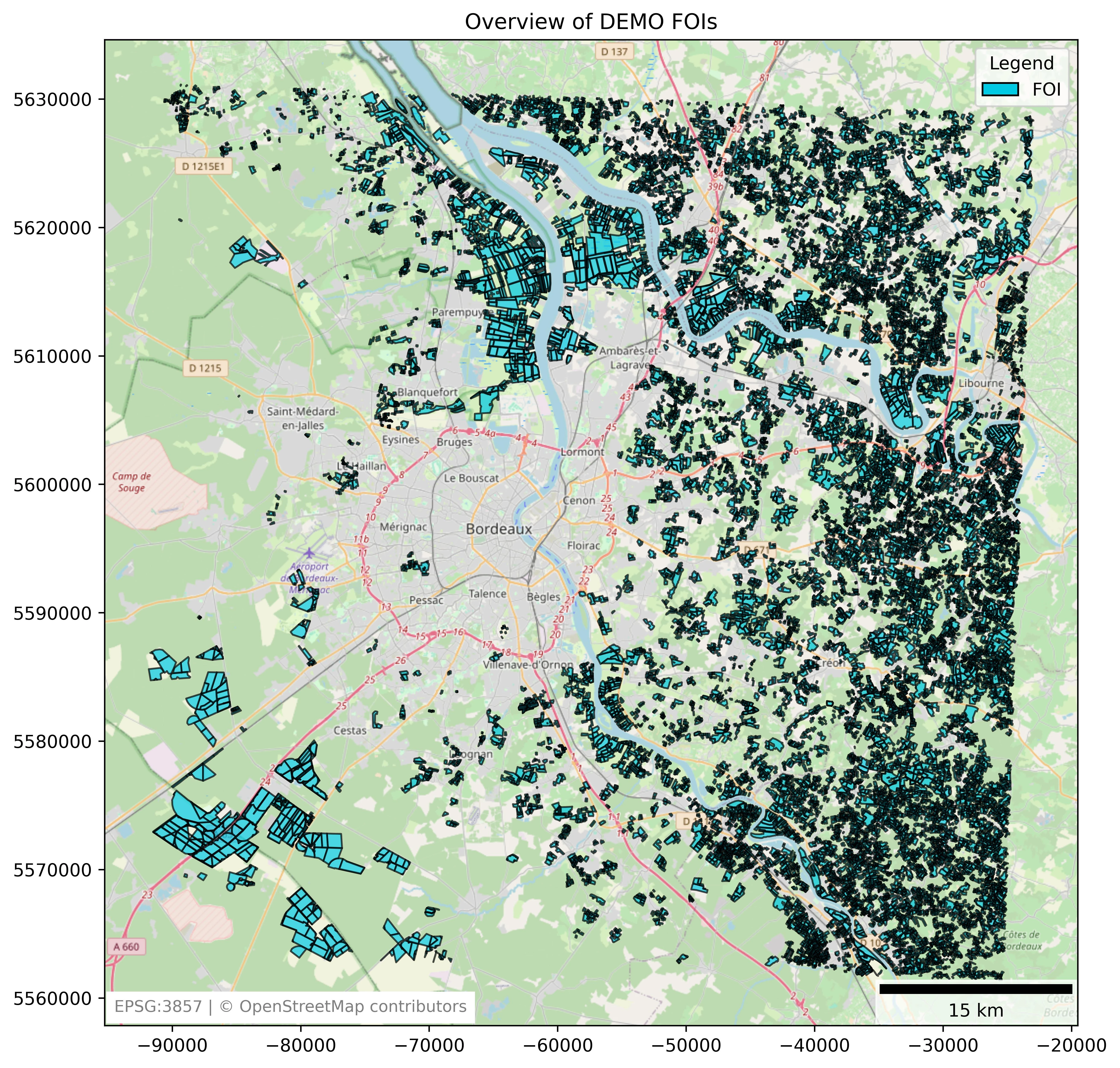
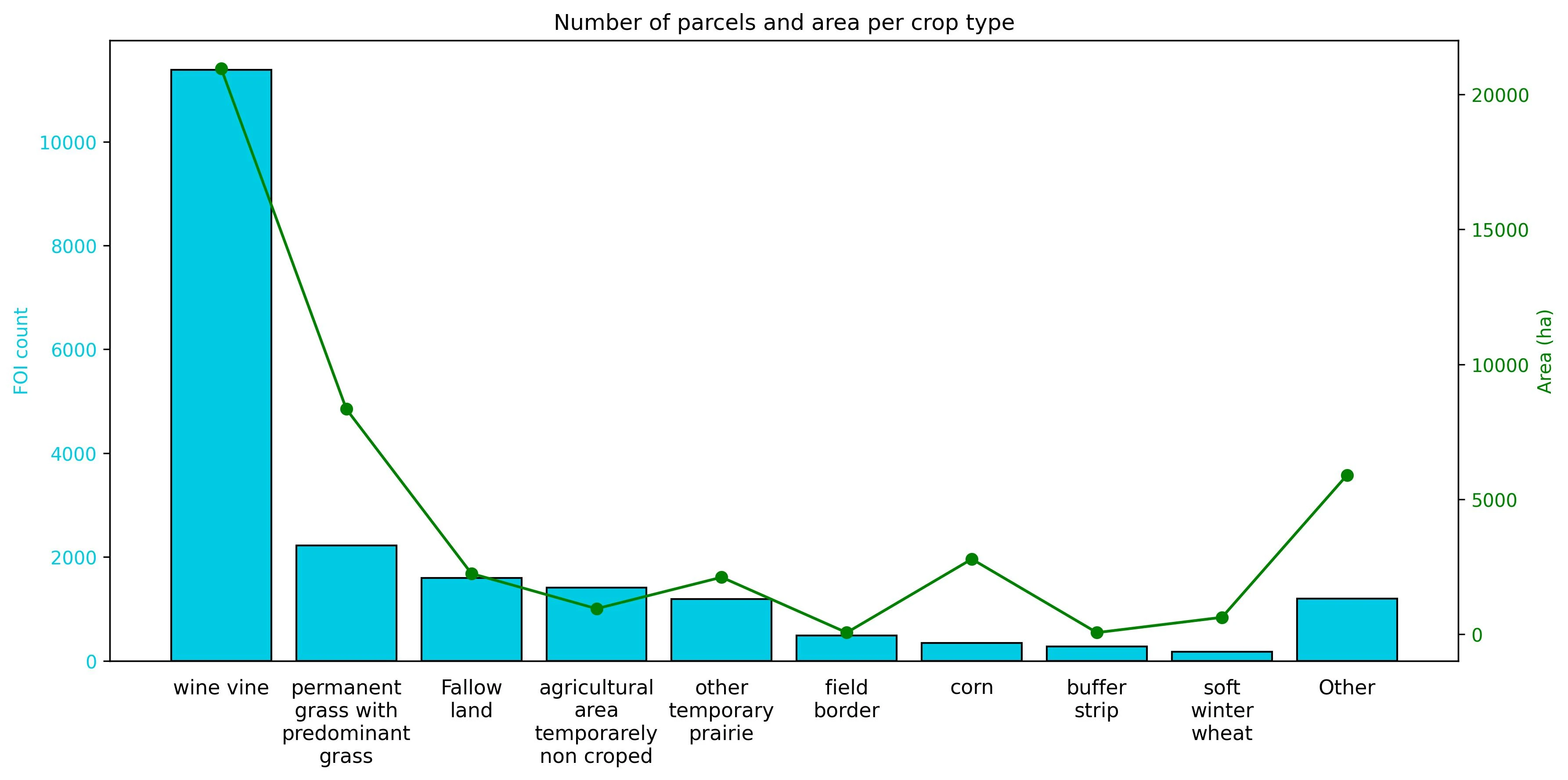
Reference data produced by the Agence de Services et de Paiement (ASP) is part of the [Registre Parcellaire Graphique (RPG)](https://geoservices.ign.fr/rpg), a French geographic database providing detailed information on agricultural parcels. This data is used to process agricultural aid applications under the Common Agricultural Policy (CAP) in France. The publicly available RPG data includes: * Geographic information on agricultural parcels, which are the basic units of land declared by farmers. * Main crop types associated with each parcel. The reference data consists mainly of vineyards and permanent grasslands. Below you can see the distribution of the most common crops. ![Distribution of FOI's](/data/area-monitoring/barplot_crops.webp)
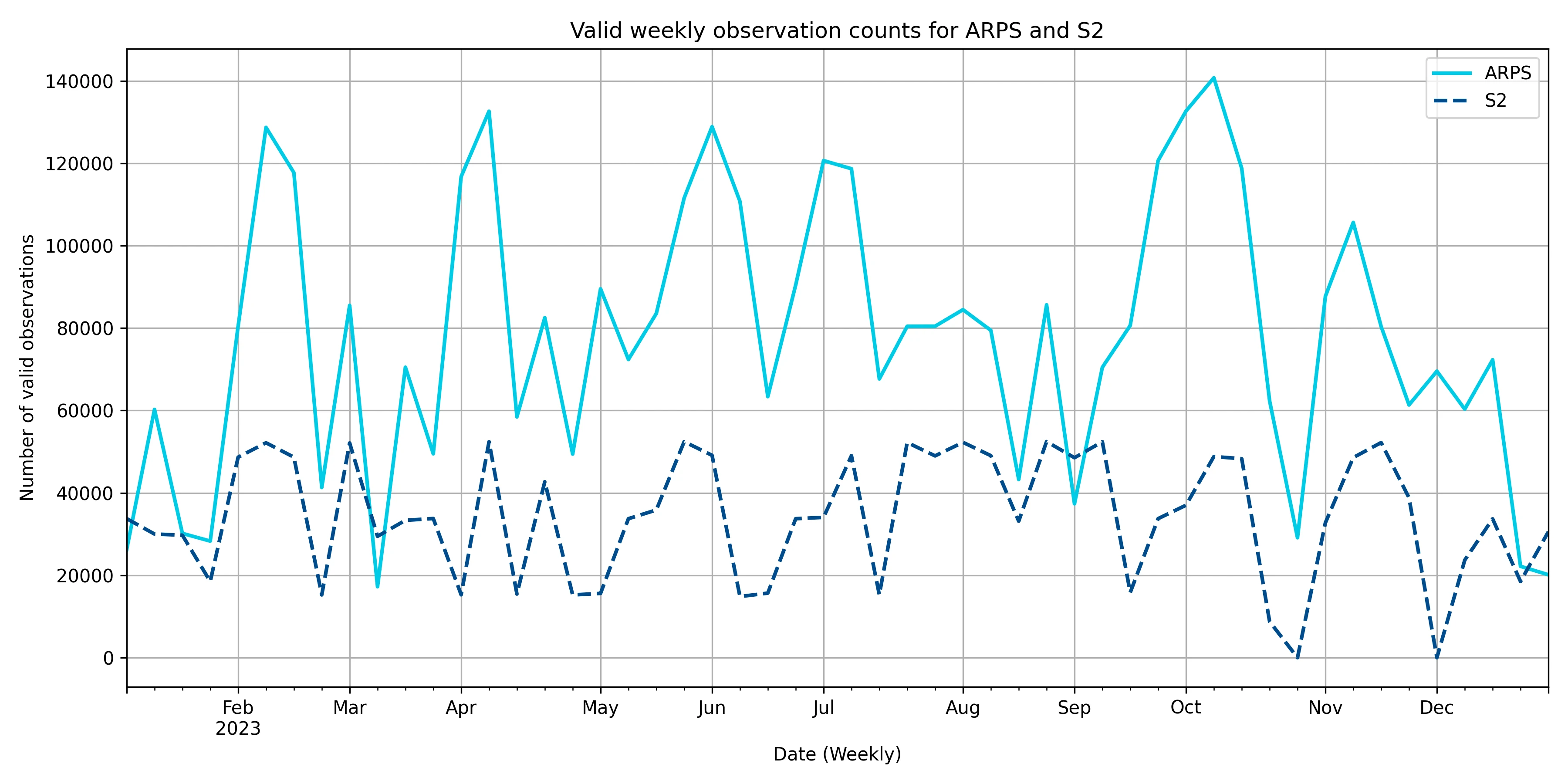
Signals were downloaded from two sources: Sentinel-2 (S2) and Analysis Ready PlanetScope (ARPS) for 2023. Sentinel-2 provides freely available 10m resolution multispectral imagery, while ARPS offers ready-to-use data from PlanetScope satellites, enabling efficient and comprehensive monitoring of agricultural parcels with 3m resolution. Compared to S2, ARPS—with its lower revisit time—produced more valid observations (for example, observations that are cloudless and not outliers), as shown in the image below. This difference was especially noticeable during the cloudy autumn months. ![Comparison of number of valid observations for 2023 within demo area](/data/area-monitoring/weekly_valid_count.webp)
In general, this difference can result in missed events or observations. The overview below for 2023 shows the percentage of FOIs that had at least one valid observation. With ARPS, there were only two weeks—one in January and one in March—when no valid observations were available due to clouds, compared to nine such weeks with Sentinel-2. ![% of FOIs with valid observations throughout 2023](/data/area-monitoring/weekly_valid_polyid_percentage.webp)
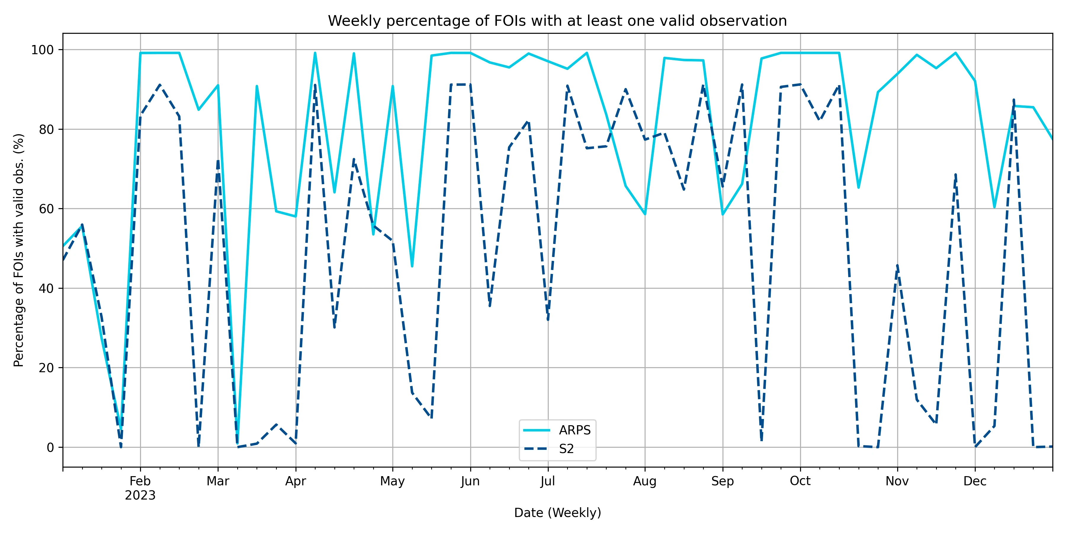
--- Copy for LLM[View as Markdown](https://docs.planet.com/data/area-monitoring/applications/) # Applications In this chapter, we will take a look at the following applications: * [Area Monitoring Application](https://docs.planet.com/data/area-monitoring/applications/area-monitoring-browser.md) for viewing the markers and Traffic Light System (TLS) decisions, * [Expert Judgement Application](https://docs.planet.com/data/area-monitoring/applications/expert-judgement-application.md) for review of the markers and TLS calculations and providing experts' evaluation of the TLS results, * [Geotagged Photo Application](https://docs.planet.com/data/area-monitoring/applications/geotagged-photo-application.md) for communication between the Paying Agency and the farmer, * [Admin Application](https://docs.planet.com/data/area-monitoring/applications/admin-application.md) for configuration of area monitoring system and checking of its status. --- Copy for LLM[View as Markdown](https://docs.planet.com/data/area-monitoring/applications/admin-application/) # Admin Application ## Overview The **Admin Application** provides a centralized place to: * check the status of the area monitoring system * create and configure scopes * configure area monitoring system components (for example, the reference data, the signals, the markers and the traffic light system) for a specific scope. Therefore, this user guide assumes that: * you have a solid understanding of the [Area Monitoring](https://docs.planet.com/data/area-monitoring.md). * you have been granted access to the **Admin Application**. Once you are logged in you will see the below user interface. ![](/data/area-monitoring/applications/admin-application/admin-app-ui.webp) The **Admin Application** user interface consists of the following components: | Name | Description | | ----------------------------------------- | ------------------------------------------------------------------------------------------------------------------------------------------------------------------------------------------------------------------------------------------------------------------------------------------------------------------ | | **Drop-down arrow** next to the **Scope** | Allows you to view a list of scopes you have access to. Selecting a scope will expose the conditional sections. | | **Add new** button | Allows you to [create a scope](#create-a-scope). | | **System overview** section | Shows the following details about the services that are part of Area Monitoring [applications](https://docs.planet.com/data/area-monitoring/applications.md): service name, base URL, version information, build information, API documentation presented as a hyperlink and status information. | | **Administration** section | Allows you to:
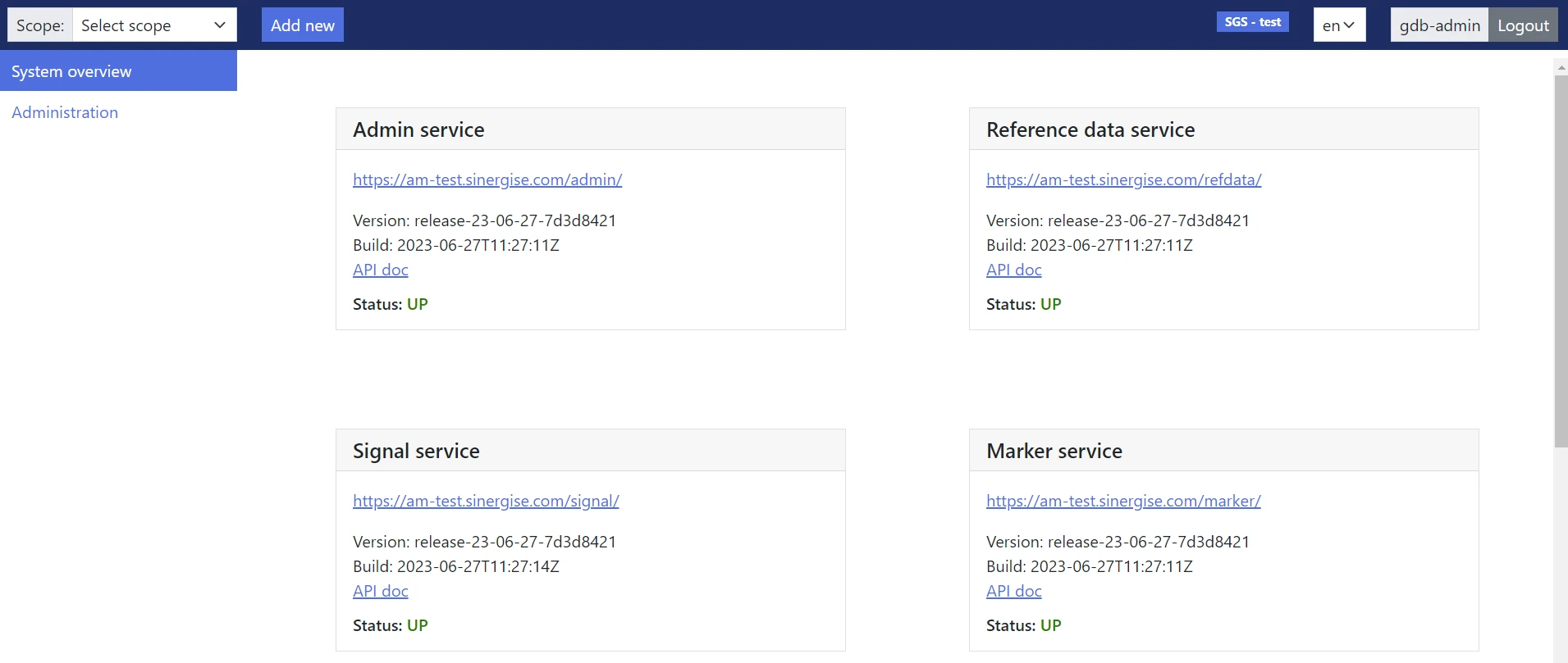
- [provide](#credentials) the credentials that will be used to access to the secured S3 bucket that you created
- [provide](#credentials) the Sentinel Hub **Client ID** and **Client Secret**
- [manage the configurations](#configuration) of different applications and services. | | **Scope Configuration** section | Shows details about the selected scope. | | **Reference Data** section | Allows you to [manage the Code lists](#code-lists) listed in this section and to [import the reference data](#import-reference-data-from-a-geopackage-file). | | **Signal** section | Allows you to [manage the Code lists](#code-lists) listed in this section and to [configure the subscriptions](#subscription) for signals retrieval. | | **Marker** section | Allows you to [manage the Code list](#code-lists) listed in this section. | | **Traffic light** section | Allows you to [manage the Code lists](#code-lists) listed in this section. | ## Create a scope ![](/data/area-monitoring/applications/admin-application/create-a-scope.webp) 1. Click **Add new**. 2. In the **Scope** field, enter the [scope ID](https://docs.planet.com/data/area-monitoring/common.md#scope). > The entered scope ID should match the scope specified in the GeoPackage file from which you will import the reference data. 3. In the **SRID** field, enter the SRID (spatial reference identifier) data, which is an EPSG code. > The entered EPSG code should match the EPSG code specified in the GeoPackage file from which you will import the reference data. 4. Click **Create**. ## Credentials This feature enables you to provide: * the S3 credentials that will be used to access the bucket that you created * the Sentinel Hub **Client ID** and **Client Secret**. ![](/data/area-monitoring/applications/admin-application/s3-credentials.webp) 1. Get your Sentinel Hub **Client ID** and **Client Secret**. For more information about how to get your Sentinel Hub **Client ID** and **Client Secret** please check [these instructions](https://docs.planet.com/guides/beginners-guide.md#get-your-client-credentials) or [this part of the tutorial video](https://www.youtube.com/watch?v=CBIlTOl2po4\&t=1760s). 2. Select the appropriate **Scope**. 3. Go to the **Administration** section. 4. Go to the **Credentials** tab. 5. Enter the S3 bucket credentials, the Sentinel Hub **Client ID** and **Client Secret** in JSON format. 6. Click **Save**. ## Configuration This feature enables you to [create](#create-a-configuration) and [edit](#edit-a-configuration) the configurations of different applications and services. ### Create a configuration ![](/data/area-monitoring/applications/admin-application/create-configuration.webp) 1. Select the appropriate **Scope**. 2. Go to the **Administration** section. 3. Go to the **Configuration** tab. 4. Click **Create**. 5. In the **Key** field, enter a key. 6. Choose a content type from the drop-down menu. 7. In the **Validator** field, specify a validator. 8. Enter the configuration data. 9. Click **Save**. ### Edit a configuration 1. Select the appropriate **Scope**. 2. Go to the **Administration** section. 3. Go to the **Configuration** tab. 4. Click on the details of the desired configuration. 5. Edit any of the other editable fields that display. See [Create a configuration](#create-a-configuration) for an explanation of the fields. 6. Click **Save**. ## Code lists Managing Code lists include actions such as [adding](#add-code-list-records) records to a Code List, [modifying](#edit-a-code-list-record) the record details and [deleting](#delete-a-code-list-record) records from a Code List. ### Add code list records You can add records to a Code list using: * [JSON](#add-a-code-list-record-using-json) * [templates](#add-code-list-records-using-templates) * [CSV file](#add-code-list-records-using-a-csv-file) #### Add a code list record using JSON ![](/data/area-monitoring/applications/admin-application/creating-using-json.webp) 1. Select the appropriate **Scope**. 2. Go to the **Reference Data** | **Signal** | **Marker** | **Traffic light** section. 3. In the **Code Lists** tab, click on the desired Code list title. 4. Click **Add new record**. 5. Enter the record data in JSON format and click **Add**. note Note that a JSON key represents a header row value in a CSV file (see [Add code list records using a CSV file](#add-code-list-records-using-a-csv-file) for more details). #### Add code list records using templates In the sections **Signal** and **Marker** you can use templates to populate in bulk the records of the Code lists with data from predifined Code list templates for each Sentinel Hub (SH) collection. > Any template from the **Signal** section populates the following dependent Code lists: * `sh-collection-types` listed in **Code Lists** tab from the **Signal** section * `signal-types` listed in **Code Lists** tab from the **Signal** section * `pixelation-types` listed in the **Code Lists** tab from the **Reference Data** section. > Any template from the **Marker** section populates the `marker-types` Code list listed in the **Code Lists** tab from this section. ![](/data/area-monitoring/applications/admin-application/creating-using-templates.webp) 1. Select the appropriate **Scope**. 2. Go to the **Signal** | **Marker** section. 3. Go to the **Templates** tab. 4. Choose a collection from the drop-down menu. > In the drop-down menu from the **Signal** section are listed the collections types which are not included in the `sh-collection-types` Code list. > > In the drop-down menu from the **Marker** section will be listed the collections which are included in the `sh-collection-types` Code list. 5. In the **SentinelHub collection source** field, enter the BYOC collection source if this was not auto-populated. 6. Click **Add**. #### Add code list records using a CSV file You can use a comma-separated values (CSV) file that contains information about the new Code list records you want to create in bulk. note Note that we recommend this method for adding records for the following code lists: `crops`, `agricultural-practice`, `foi-types`, `land-uses`, `schemes`, `soil-types`, `traffic-light-colours`, `decisions`, `event-types`, `judgement-reasons` and `lanes`. ![](/data/area-monitoring/applications/admin-application/creating-using-a-csv-file.webp) 1. Select the appropriate **Scope**. 2. Go to the **Reference Data** | **Signal** | **Marker** | **Traffic light** section. 3. In the **Code Lists** tab, click on the desired Code list title. 4. Click **Import CSV**. 5. In the **Select CSV file** pop-up window, click **Browse**, choose the CSV file and click **Import**. To successfully import a CSV, the content must adhere to these rules: * The CSV file must consist of a header row that names the columns and multiple rows of values that are separated by semicolons (;) (or other characters). * Each row of values is a Code list record. * Header row values must match the field values listed in the below CSV file requirements that are provided for the Code lists for which the recommended method to add records is via a CSV file. * Header row values are not required to be in the order listed, just make sure that the column header is over the appropriate information in each respective column. **The CSV file requirements** for the code lists for which the recommended method to add records is via a CSV file: | Field | Data type | Required | Description | Code List | | ---------------------- | --------- | -------- | ------------------------------------------------------------------------------------------------------------------------------------------------------------------------------------------------------------------------------------------------------------------------------------------------ | ---------------------------------------------------------------------------------------------------------------------------------------------------------------------- | | `code` | string | YES | Record's short unique code (use uppercase letters `[A-Z]`, numbers `[0-9]`, `_`, `-`) | `crops`, `agricultural-practice`, `foi-types`, `land-uses`, `schemes`, `soil-types`, `traffic-light-colours`, `decisions`, `event-types`, `judgement-reasons`, `lanes` | | `names.` | string | NO | - Record's long name in given language
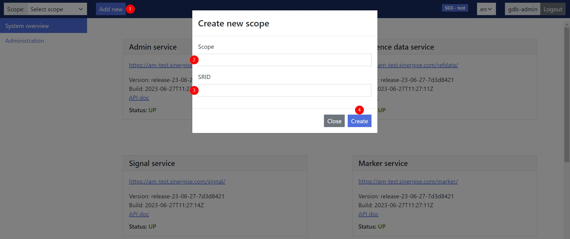
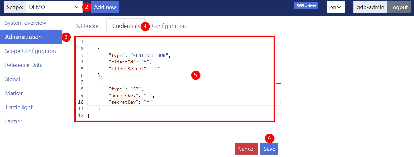
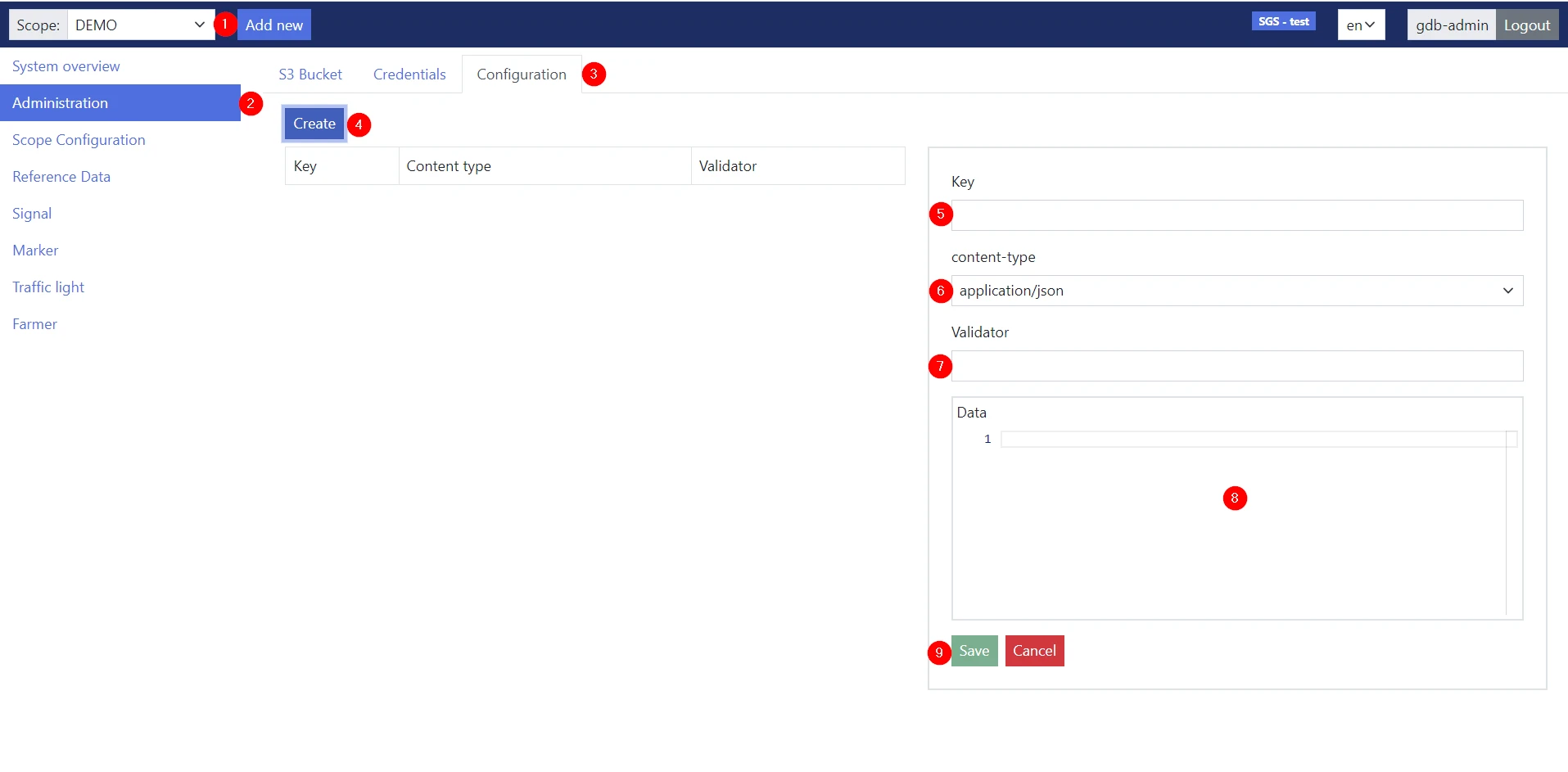
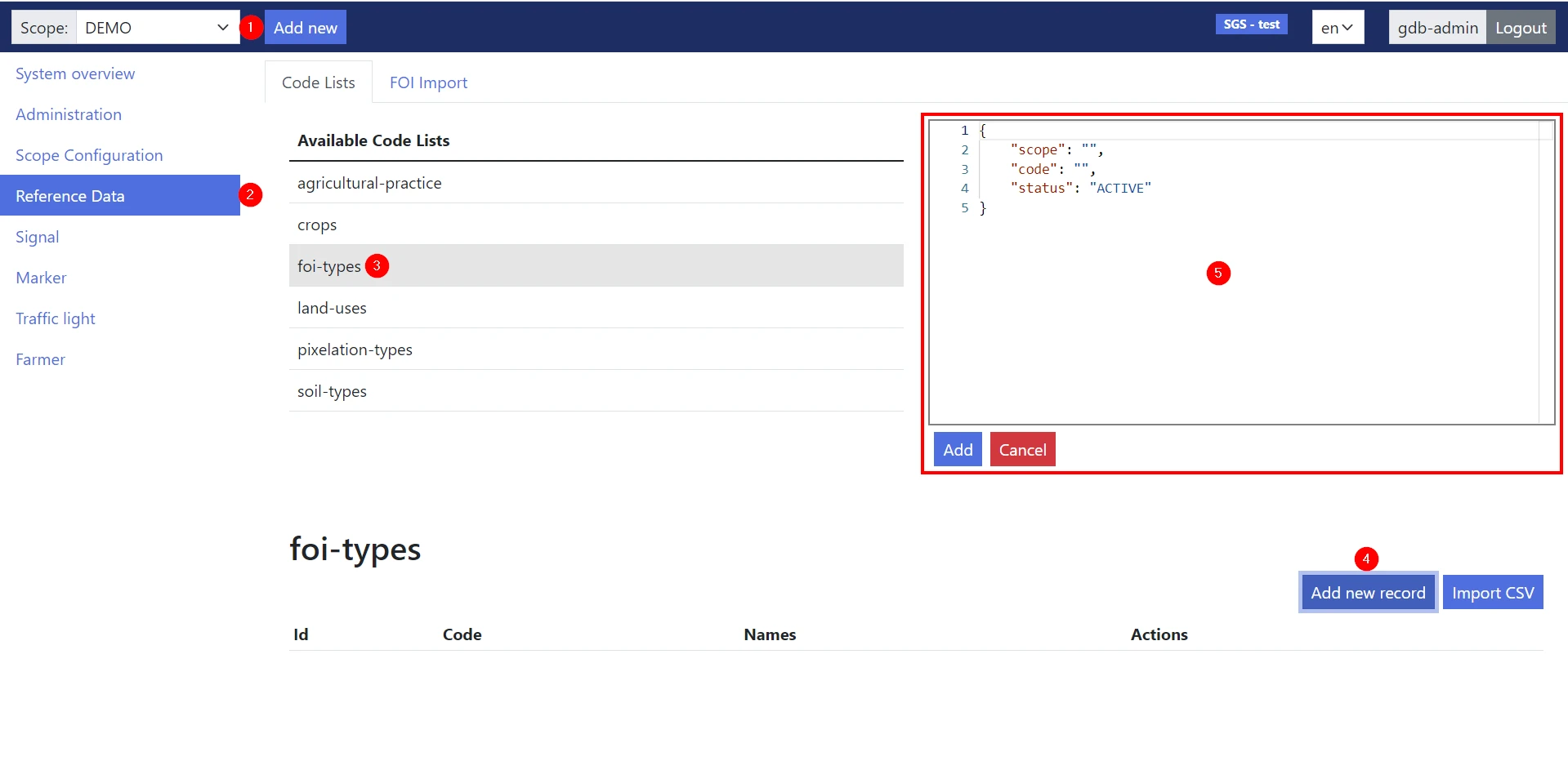
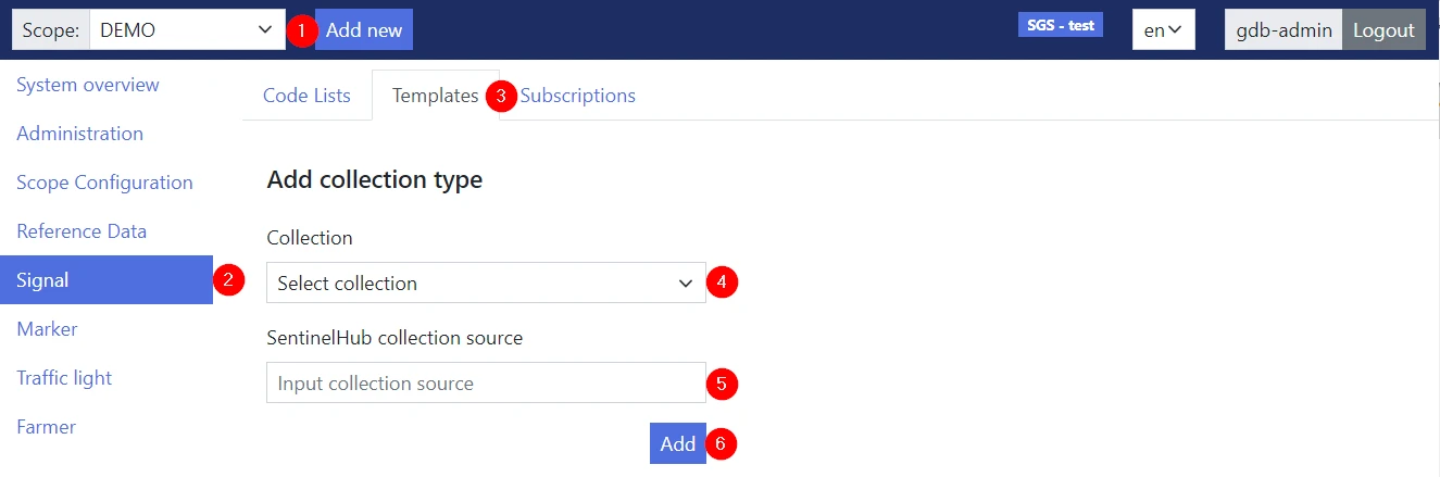
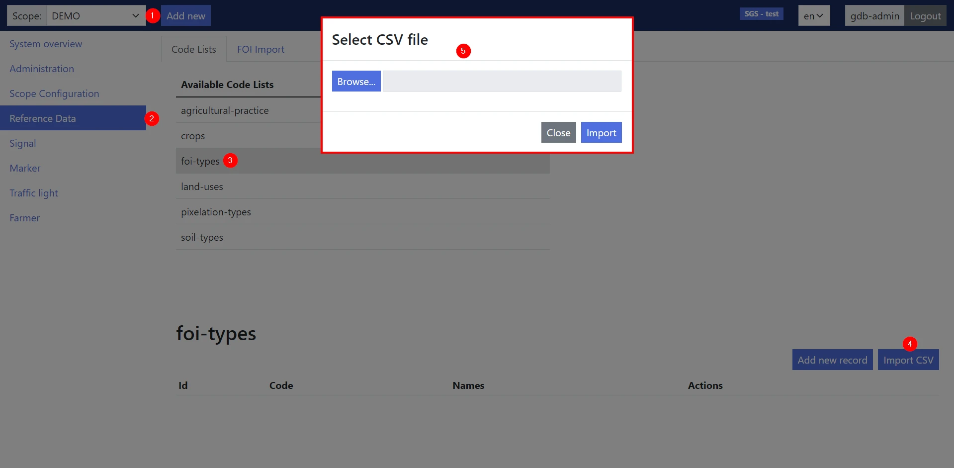
- Change `` in field name with appropriate [ISO 639 Language ID](https://www.localeplanet.com/icu/iso639.html#et) (for example, `names.en`)
- You can add names fields for several different languages (e.g. `names.en`, `names.sl`). | `crops`, `agricultural-practice`, `foi-types`, `land-uses`, `schemes`, `soil-types`, `traffic-light-colours`, `decisions`, `event-types`, `judgement-reasons`, `lanes` | | `status` | string | YES | Record's status (usually `ACTIVE` but can be `HISTORIC`). | `crops`, `agricultural-practice`, `foi-types`, `land-uses`, `schemes`, `soil-types`, `traffic-light-colours`, `decisions`, `event-types`, `judgement-reasons`, `lanes` | | `scope` | string | YES | Scope ID of the scope to which the Code list belongs. | `crops`, `agricultural-practice`, `foi-types`, `land-uses`, `schemes`, `soil-types`, `traffic-light-colours`, `decisions`, `event-types`, `judgement-reasons`, `lanes` | | `has_financial_impact` | bool | YES | Record's financial impact (`True` or `False`) | `schemes` | | `priority` | int4 | YES | Traffic light colour priority (the default is `0` ) | `traffic_light_colours` | For example, the content of the CSV file to be used for adding records to the `crops` code list should look like this: > code;names.en;names.sl;status;scope
1;buckwheat;ajda;ACTIVE;DEMO
2;sugar beet;sladkorna pesa;ACTIVE;DEMO ### Edit a Code list record ![](/data/area-monitoring/applications/admin-application/editing-using-json.webp) 1. Select the appropriate **Scope**. 2. Go to the **Reference Data** | **Signal** | **Marker** | **Traffic light** section. 3. In the **Code Lists** tab, click on the desired Code list title. 4. Click the **Edit** button next to the record to be edited. 5. Edit the JSON text and click **Save**. ### Delete a Code list record ![](/data/area-monitoring/applications/admin-application/deleting-record.webp) 1. Select the appropriate **Scope**. 2. Go to the **Reference Data** | **Signal** | **Marker** | **Traffic light** section. 3. In the **Code Lists** tab, click on the desired Code list title. 4. Click the **Delete** button next to the record to be deleted. 5. In the **Delete confirmation** pop-up window, click **Save**. ## Import reference data from a GeoPackage file This process assumes that: * you [have populated the appropriate Code lists](#code-lists) from the **Code Lists** tab of the **Reference Data** section: * `foi-types` (mandatory) * `crops` (mandatory if in the GeoPackage file is specified the `crop_code`) * `land-uses` (mandatory if in the GeoPackage file is specified the `land_use_code`) * the GeoPackage adheres to the specifications * you have uploaded the GeoPackage to a S3 bucket for which you [provided the credentials](#credentials). ![](/data/area-monitoring/applications/admin-application/import-reference-data.webp) 1. Select the appropriate **Scope**. 2. Go to the **Reference Data** section. 3. Go to the **FOI Import** tab. 4. Choose a FOI type from the drop-down menu which lists the `foi-types` Code list records. 5. In the **Geopackage path** field enter the file’s S3 path. 6. In the **Geopackage FOI table name** field enter the name of the GeoPackage table with the reference data to import. 7. In **Geopackage additional attributes** field enter the name of the attribute specified in addition to the attributes from the GeoPackage specifications for the reference data. In case of multiple additional attributes, the names of the columns should be separated by a `,` (comma) for example, Att1, att2, etc. 8. Click **Import**. ## Subscription This feature enables you to specify the details required for retrieval of signals. ### Create a subscription This process assumes that: * you [have imported the reference data](#import-reference-data-from-a-geopackage-file) * you [have populated the Code lists](#code-lists) from the **Code Lists** tab from the **Signal** section * you have uploaded to the S3 bucket for which you [provided the credentials](#credentials) the CSV file with the FOI IDs for which you want to retrieve SH collection signals * the signals will be downloaded to the S3 bucket for which you [provided the credentials](#credentials) . ![](/data/area-monitoring/applications/admin-application/create-subscription.webp) 1. Select the appropriate **Scope**. 2. Go to the **Signal** section. 3. Go to the **Subscriptions** tab. 4. Click **Create new**. 5. Select a SH collection type from the drop-down menu which lists the `sh-collection-types` Code list records. 6. In **FOI filter** field enter the filter criteria if you want to retrieve SH collection signals only for the FOIs that match the entered criteria. > For the filter criteria refer to the API documentation for the `/refdata/{scope}/fois/search` API endpoint under the `foi-controller` resource that can be accessed from the API documentation hyperlink of the `Reference data service` shown in the **System overview** section. 7. In **FOI ID's CSV path** field enter the file’s S3 path with the FOI IDs for which you want to retrieve the SH collection signals. 8. Enter the time interval for which you want to retrieve the SH collection signals. 9. Select the checkbox next to the SH collection signals you want to compute. 10. In **S3 subscription path** field enter the S3 bucket path where will be downloaded to the retrieved signals. 11. Configure advanced evalscript options such as `mosaicking`, `custom datamasks` and `preProcessScenes`. For more information, see the [Evalscipts](https://docs.planet.com/develop/evalscripts/) section. 12. Click **Save**. ### Edit a subscription ![](/data/area-monitoring/applications/admin-application/edit-subscription.webp) 1. Select the appropriate **Scope**. 2. Go to the **Signal** section. 3. Go to the **Subscriptions** tab. 4. Click on the details of the desired subscription. 5. Edit any of the other editable fields that display. When changing the `Interval start` and `Interval end` keep in mind that subscriptions are only incremental in time. That means that if any signals were already downloaded (DONE signal packages exist) that `Interval start` should not be changed and `Interval end` can only be incremented in time. See [Create a subscription](#create-a-subscription) for an explanation of the fields. 6. Click **Save**. --- Copy for LLM[View as Markdown](https://docs.planet.com/data/area-monitoring/applications/area-monitoring-browser/) # Area Monitoring Application Area Monitoring App is a web application that aggregates data from connected systems in order to provide the ability for viewing the information on markers and Traffic Light System (TLS) decisions of a Feature of Interest (FOI) and is part of the Area Monitoring System. ## Basic navigation At the left of the interface, you can select the scope (DEMO\_FR23 in this case), limit the timerange of the observations, observations layer and select marker context. ![](/data/area-monitoring/applications/area-monitoring-browser/dashboard-left.webp) ### FOI selection #### Select one of the suggested FOIs 1. Select the **scope** from the drop-down list. > Scope defines the geographical data and temporal intervals that will be available for selection and restricts the options in subsequent filters. Note that with the trial access, you will be limited to the `DEMO` scope. 2. Click on the `Suggest FOIs` button ![](/data/area-monitoring/applications/area-monitoring-browser/suggest-fois.webp) This will open a pop-up window with a list of suggested FOIs. ![](/data/area-monitoring/applications/area-monitoring-browser/suggested-fois.webp) 3. (Optional) Filter the suggested FOIs by FOI type, land use or crop type. 4. Select a **FOI** from the list. #### Select a FOI with a specific id 1. Select the **scope** from the drop-down list. 2. Select the **FOI type** from the drop-down list. > FOI type selection is not needed if you provide the full FOI reference Id (for example, `DEMO.FOI.6999931001`) in the input field next to the FOI type drop-down. Note that you have only one type available in the `DEMO` scope, for example, `AP` - agricultural parcel. 3. Enter the **FOI ID**. 4. Press the **Search** button. ### Temporal selection 1. (Optional) Shorten the default timespan and press the **Search** button. When a valid FOI ID is entered, the timespan will be populated automatically and override the user's setting. 2. (Optional) Select the **Marker context** from the drop-down menu. > Different marker contexts are available in case of several calculations of the markers within the season. Note that with the trial access, you will be limited to one marker context. All of the information available for the selected FOI is displayed in several widgets. ![](/data/area-monitoring/applications/area-monitoring-browser/all-sections.webp) ### Collapse or expand widgets (Optional) Click on the corresponding section header with a collapse/expand arrow to collapse or expand widgets located within the same section. ![](/data/area-monitoring/applications/area-monitoring-browser/overview-timelaps-signals-collapsed.webp) ## Widgets ### FOI **FOI** widget shows the general information about the selected FOI. ![](/data/area-monitoring/applications/area-monitoring-browser/overview-section.webp) ### Claims **Claims** widget shows all the claims associated with the selected FOI. The last column shows the latest assigned traffic light decision, if available, and the TLS diagram used to make the decision. ![](/data/area-monitoring/applications/area-monitoring-browser/tls-diagram-button.webp) Click on the `Diagram` buttom opens in a new browser tab the TLS diagram used to make the latest traffic light decision assigned to the claim. To show/hide all the traffic light decisions assigned to a specific claim, click on expand/collapse arrow. ![](/data/area-monitoring/applications/area-monitoring-browser/claims-section.webp) ### Markers The Markers widget group shows the following widgets: `Summary`, `Land cover group`, `Distance`, `Similarity`, `Crop group` and `Pixel Mowing`. Each of these can display information from more than one data source, if available (for example, S2 = Sentinel-2, PF = PlanetFusion). #### Summary ![](/data/area-monitoring/applications/area-monitoring-browser/markers-rows.webp) **Summary** widget displays information for the markers listed below: * `Land cover group` - predicted land cover group and confidence in the prediction * `Crop group` - predicted crop group and confidence in the prediction * `Similarity` - most similar crop type according to the similarity marker and its score (the lower the number, the more similar) * `Distance` - most similar crop type according to the distance marker and its score (the lower the number, the more similar) * `Bare soil` - number of bare soil observations within the scope timespan * `Mowing` - number of detected mowing events within the scope timespan * `Mowing (pixel level)` * first three numbers (1 / 6 / 224 on the screenshot above) present: * largest number of spatially connected pixels with detected mowing events, * number of all pixels with mowing detected, * number of full pixels in FOI pixelized geometry. * the 2 numbers on the right (0.4% / 2.7% on the screenshot above) present: * largest number of spatially connected pixels with detected mowing events divided by total number of pixels, * number of all pixels with mowing detected divided by total number of pixels. * `NDVI mean` - mean NDVI value of all valid observations per FOI within the scope timespan * `Homogeneity` - predicted homogeneity (or non-homogeneity) and confidence in the prediction #### Land cover group and Crop group Under the **Land cover group** widget, classification scores for all land cover classes are presented graphically (see [Marker Scores](https://docs.planet.com/data/area-monitoring/visualizations/marker-scores.md) visualization component for more information). The predicted land cover group is rendered in green. If the declared land cover is not the same as the predicted one, it is rendered in darker blue color. The same principle is in use for presenting classification scores for all crop groups in the **Crop group** widget. ![](/data/area-monitoring/applications/area-monitoring-browser/land-cover-group.webp) #### Distance and Similarity Under the **Distance** widget, the scores for all crops are presented graphically (see [Marker Scores](https://docs.planet.com/data/area-monitoring/visualizations/marker-scores.md) visualization component for more information). The most similar crop is rendered in green. If the declared crop is not the most similar one, it is rendered in darker blue color. The same principle is in use for presenting similarity marker scores in the **Similarity** widget. ![](/data/area-monitoring/applications/area-monitoring-browser/distance.webp) ### Traffic Lights In the **Traffic Lights** widget, you can see all traffic light calculations performed for the selected FOI. ![](/data/area-monitoring/applications/area-monitoring-browser/tls-diagram-button.webp) Clicking the `Show diagram` button displays the TLS diagram in a new browser tab. ![](/data/area-monitoring/applications/area-monitoring-browser/tls-tab.webp) ### Observations In the **Observations** widget, you can see all available image chips for the selected FOI and selected layer (by default, only valid observations are shown). ![](/data/area-monitoring/applications/area-monitoring-browser/observations-section.webp) In the options row, you can choose: * the desired layer, * the number of columns used for laying out observation images, * padding of the image chip around FOI geometry and * whether images are filtered using the valid signal or not. ![](/data/area-monitoring/applications/area-monitoring-browser/observations-options.webp) ![](/data/area-monitoring/applications/area-monitoring-browser/open-image-chip-button.webp) Clicking the image chip displays it in a new pop-up window that can be dragged or resized. ### Map In the **Map** Widget, you can see the selected FOI and the neighboring FOIs. ![](/data/area-monitoring/applications/area-monitoring-browser/map-section.webp) If you move the map around, all available FOIs in the area will be displayed, to a certain zoom level. Clicking on any of the FOIs shown on the map will display the data related to that FOI in all widgets. ![](/data/area-monitoring/applications/area-monitoring-browser/map-options.webp) In the top right, you can select various `Map options`: 1. Choose if you wish to display the selected **FOI** with a yellow outline (so it stands out compared to other FOIs in the area) or not. ![](/data/area-monitoring/applications/area-monitoring-browser/map-options-select-foi.webp) 2. Select the background **Layer** - Aerial Photography, S2 True Color, S2 False Color, etc. If a satellite imagery is selected as a background, you can set the timestamp by clicking on the specific date in the `Signals Markers Visualization` widget. ![](/data/area-monitoring/applications/area-monitoring-browser/map-options-select-layer.webp) 3. Choose how you wish to display the neighbouring **FOIs**: show them or not, colour them by crop type or land use type, display the labels for the crop type or land use type. ![](/data/area-monitoring/applications/area-monitoring-browser/map-options-select-fois.webp) 4. Set **Filters** to display the FOIs matching the specified criteria with a blue outline so that they stand out compared to other FOIs (white outline) in the area. A filter can be applied to crop type, land use type, number of pixels or to a combination of these properties. ![](/data/area-monitoring/applications/area-monitoring-browser/map-options-filter-fois.webp) ### Timelapse In the **Timelapse** widget (see [Timelapse](https://docs.planet.com/data/area-monitoring/visualizations/timelapse.md) visualization component for more information), you can see the timelapse of the selected FOI's image chips for the selected layer. You can download the timelapse as a GIF file. You can either play the timelapse or navigate from one image chip to the next one. ![](/data/area-monitoring/applications/area-monitoring-browser/timelapse-section.webp) ### Signals Markers Visualizations In the **Signals Markers Visualization** widget (see [Signal Marker Visualization](https://docs.planet.com/data/area-monitoring/visualizations/signal-marker-visualization.md) component for more information), you can see the graph of all available and selected signals and markers for the selected FOI and for the marker context in the selected period. ![](/data/area-monitoring/applications/area-monitoring-browser/signals-markers-visualizations-section.webp) ![](/data/area-monitoring/applications/area-monitoring-browser/csv-button.webp) Clicking on the `CSV` button downloads all available data in a CSV format. ![](/data/area-monitoring/applications/area-monitoring-browser/json-button.webp) Clicking on the `JSON` button displays all available data in JSON format in a new browser tab. ![](/data/area-monitoring/applications/area-monitoring-browser/settings.webp) Settings are available by clicking on the "Settings" icon in the bottom right. Here you can choose between several options of where the tooltip should be placed when hovering over points in the timeline. ![](/data/area-monitoring/applications/area-monitoring-browser/legend.webp) The Legend is below the graph, showing which signals and markers are available. **Left clicking** on a label will toggle on and off the items shown on the graph. If indicated by a colored square, the item is shown on the graph. **Ctrl/cmd + Left clicking** on a label will toggle on and off the items included in the tooltip. If indicated by bold text, the item is included in the tooltip. ## Sentinel 2 visualisations You can choose between different visualitations of the Sentinel 2 imagery in the `Observations`, `Map` and `Timelapse` widgets. ### S2 True color ![](/data/area-monitoring/applications/area-monitoring-browser/layers-S2-true-color.webp) True color composite: Sentinel-2 has 13 bands. True color composite uses visible light bands red, green and blue in the corresponding red, green and blue color channels, resulting in a natural colored product, that is a good representation of the Earth as humans would see it naturally. [More details](https://custom-scripts.sentinel-hub.com/sentinel-2/true_color/) ### S2 False color v1 False color composite: The false color composite using near infrared, red and green bands is most commonly used to assess plant density and health, since plants reflect near infrared and green light, while they absorb red. ![](/data/area-monitoring/applications/area-monitoring-browser/layers-S2-false-color1.webp) [More details](https://custom-scripts.sentinel-hub.com/sentinel-2/false_color_infrared/) ### S2 False color v2 False color composite with enhanced contrast: The false color composite using near infrared, red and green bands, but other color channels than the S2 False color v1. ![](/data/area-monitoring/applications/area-monitoring-browser/layers-S2-false-color2.webp) [More details](https://custom-scripts.sentinel-hub.com/sentinel-2/false_color_infrared/) ### S2 NDVI - Normalized Difference Vegetation Index (NDVI) The normalized difference vegetation index is a simple, but effective index for quantifying green vegetation. It is a measure of the state of vegetation health based on how plants reflect light at certain wavelengths. The value range of the NDVI is -1 to 1. Negative values of NDVI (values approaching -1) correspond to water. Values close to zero (-0.1to 0.1) generally correspond to barren areas of rock, sand, or snow. Low, positive values represent shrub and grassland (approximately 0.2 to 0.4), while high values indicate temperate and tropical rainforests (values approaching 1). ![](/data/area-monitoring/applications/area-monitoring-browser/layers-S2-NDVI.webp) [More details](https://custom-scripts.sentinel-hub.com/sentinel-2/ndvi/) ### S2 CCC - Canopy Chlorophyll Content CCC (Canopy Chlorophyll Content \[$μg / cm ^ 2$]) is calculated here as the product of the leaf area index (LAI) with the leaf cholrophyll content (Cab). Visualized as an interval from 0-900. ![](/data/area-monitoring/applications/area-monitoring-browser/layers-S2-CCC.webp) [More details](https://custom-scripts.sentinel-hub.com/sentinel-2/ccc/) ### S2 EVI - Enhanced Vegetation Index In areas of dense canopy cover, where leaf area index (LAI) is high, the blue wavelengths can be used to improve the accuracy of NDVI, as it corrects for soil background signals and atmospheric influences. Values description: The range of values for EVI is -1 to 1, with healthy vegetation generally around 0.20 to 0.80. ![](/data/area-monitoring/applications/area-monitoring-browser/layers-S2-EVI.webp) [More details](https://custom-scripts.sentinel-hub.com/sentinel-2/evi/) ### S2 LAI - Leaf Area Index LAI is a dimensionless index measuring the one-sided green leaf area over a unit of land \[$m^2 / m^2$]. Visualized as an interval from 0-3. ![](/data/area-monitoring/applications/area-monitoring-browser/layers-S2-LAI.webp) [More details](https://custom-scripts.sentinel-hub.com/sentinel-2/lai/) ### S2 NDWI - Normalized Difference Water Index (NDWI) The normalized difference water index is most appropriate for water body mapping. Values of water bodies are larger than 0.5. Vegetation has smaller values. Built-up features have positive values between zero and 0.2. ![](/data/area-monitoring/applications/area-monitoring-browser/layers-S2-NDWI.webp) [More details](https://custom-scripts.sentinel-hub.com/sentinel-2/ndwi/) ### S2 Moisture index (NDMI) NDMI is a normalized difference moisture index, that uses NIR and SWIR bands to display moisture. In short, NDMI is used to monitor changes in water content of leaves. ![](/data/area-monitoring/applications/area-monitoring-browser/layers-S2-NDMI.webp) [More details](https://custom-scripts.sentinel-hub.com/sentinel-2/ndmi/) ### S2 NDSI - Normalised Difference Snow Index (NDSI) The Sentinel-2 normalised difference snow index can be used to differentiate between cloud and snow cover as snow absorbs in the short-wave infrared light, but reflects the visible light, whereas cloud is generally reflective in both wavelengths. Snow cover is represented in bright vivid blue. ![](/data/area-monitoring/applications/area-monitoring-browser/layers-S2-NDSI.webp) [More details](https://custom-scripts.sentinel-hub.com/sentinel-2/ndsi/) ### S2 CL\_GREEN\_V2 S2 CL\_GREEN\_V2 Chlorophyll Index visualisation is tailored for monitoring agricultural areas by visualizing the chlorophyll content in vegetation. Chlorophyll levels are a key indicator of plant health and vitality, making this index valuable for assessing crop conditions. For example, it shows the subtle differences in the state of the vegetation after the area was mowed. The index is mapped to a color gradient that visually represents different levels of chlorophyll content. Dark green colors indicate higher chlorophyll content, suggesting healthier, more vigorous vegetation, while light green colors represent lower chlorophyll levels. ![](/data/area-monitoring/applications/area-monitoring-browser/layers-S2-CL_GREEN_V2.webp) ### S2 baresoil mask and S2 built-up mask We have developed a set of binary land-cover classifiers that are able to give insights into the land-cover of each pixel of a FOI. These are: built-up mask, bare-soil mask, forest mask and water mask. The combination of these binary land-cover classifiers gives us our own proprietary on-demand scene classification map that can be applied to any single Sentinel-2 observation. Built-up mask (blue pixels) ![](/data/area-monitoring/applications/area-monitoring-browser/layers-S2-built-up.webp) Baresoil mask (red pixels) ![](/data/area-monitoring/applications/area-monitoring-browser/layers-S2-baresoil.webp) [More details](https://docs.planet.com/data/area-monitoring/markers/binary-land-cover-marker.md) --- Copy for LLM[View as Markdown](https://docs.planet.com/data/area-monitoring/applications/expert-judgement-application/) # Expert Judgement Application Expert Judgement Application allows to organise the work of experts to determine whether agricultural parcels comply with the Common Agricultural Policy (CAP) regulations by analyzing signals, markers, and auxiliary data. Package bundles are used to organize the work of experts. A package bundle defines a collection of task packages, including the number of task packages in the bundle, the task to be performed, and the associated agricultural parcels. A task package represents the task to be performed on the associated agricultural parcels, which can be assigned to an expert. Expert Judgement Application supports the following functionalities: * creation of packages in the administrative module with tasks for: * collection of the ground truth data, * marker validation and * traffic light review module * insight into the status of the FOIs included in the subsidy applications: * traffic light calculation results (including markers used in the calculation, model scenarios, model decisions, expert decision results and final traffic light results with transparent history overview) * review of the auxiliary data (satellite images and signals, orthophoto images, subsidy applications attribute data, etc.), * reports on several levels (per farm, per application, per marker). ## Administrative module The administrative module is the central access point for reviewing traffic lights, providing an overview of package bundles and work distribution among users. Below you can find the user interface. ![](/data/area-monitoring/applications/expert-judgement-application/Administrative.webp) Besides an overview of created bundles and packages (each user receives assigned packages in their inbox), the administration module allows detailed tracking of progress on FOI, claim, or eligibility criteria levels within the reporting tabs. An example is shown below. ![](/data/area-monitoring/applications/expert-judgement-application/Reporting_claims.webp) You can easily filter millions of FOIs, check their status, export them, or edit them using the Traffic Light Review module by simply clicking on the FOI ID from the list. As Expert App plays a central role for Paying Agencies for Traffic light decision making, it also enables creation of tasks for communication with farmers who submit claims. Check out example below. With help of this component, farmers can be notified via e-mail, SMS, or our [Geotagged Photo Application](https://docs.planet.com/data/area-monitoring/applications/geotagged-photo-application.md). ![](/data/area-monitoring/applications/expert-judgement-application/Communication.webp) Speaking of Geotagged Photo App - we can also mention that all geotagged photos can be shown in the Expert app providing experts additional information for decission making in examples where claim cannot be checked with remote sensing data. ![](/data/area-monitoring/applications/expert-judgement-application/Geotagged.webp) ## Traffic Light Review (TL) module The Traffic Light (TL) Review module offers a graphical interface for expert analysis of computed signals, markers, and auxiliary data to determine whether agricultural parcels comply with CAP regulations. Based on the expert's decision, a traffic light status is assigned. ![](/data/area-monitoring/applications/expert-judgement-application/TL_module.webp) *Example of TL review module in the action. FOI was is marked as non-compliant by our [TL model](https://docs.planet.com/data/area-monitoring/traffic-light-system/examples.md) as it is heterogenous with 2 different crops growing on it. Expert decided to confirm TL model decision. 4 different eligibility criterias were check for this claim (shown in the right task table) - agricultural use detection, homogeniety, compliance with non-agricultural land use rules and land use cross-check with tthe one defined in the claim.* note Note that all TL changes are transparently shown in TL history table clearly showing exact dates of the change with description of the trigger which caused TL color change. A detailed description of visualization components which you can see on the screenshot can be found [here](https://docs.planet.com/data/area-monitoring/visualizations.md). Once you are done with the review of all tasks, simply finish it with a click on a button and proceed with the next one. Results are now saved and you can access them anytime. # Ground truth collection (GTC) module In order to have optimal [marker results](https://docs.planet.com/data/area-monitoring/markers.md), ground truth data is of the outmost importance thus GT model idea was born. In the wizard for package bundle creation, define the labels you want to collect (whether at the observation or FOI level) and immediately start labeling. For observation-level GTC (for example, mowing or bare soil presence on a specific date), use mouse clicks. For FOI-level GTC (useful in land-use assessment), you can label even faster using keyboard shortcuts. ![](/data/area-monitoring/applications/expert-judgement-application/GTC_labeling.gif) Results of such labeling campaigns can be used as valuable research source in order to fine tune our markers so we could improve results in itterative process. ## Links [Blog post](https://medium.com/sentinel-hub/expert-judgement-application-67a07f2feac4) about Expert Judgement Application --- Copy for LLM[View as Markdown](https://docs.planet.com/data/area-monitoring/applications/geotagged-photo-application/) # Geotagged Photo Application The new CAP allows using a range of modern technologies when carrying out checks for area-based payments. Although area monitoring systems rely heavily on automated analysis of Earth observation data, they often use geotagged photos to support and complement the remote sensing methods when those do not provide conclusive results. ## About the application Geotagged Photo Application is an Android application that allows farmers to share their photos (geotagged or not) with the paying agency (PA). Since photos can be used as a proof of activity or to clarify the request, it is very important for PA to get as much information about the photo as possible, for example, whether the photo, its location or date of creation have been changed. Photos that have been altered, uploaded from external sources or were not geotagged will be marked differently, so that PA can take this into account in further decisions. ## Short description of the process The application is task oriented, and the typical usage comprises the following steps: * tasks are created in advance by the PA using the [Expert Judgement application](https://docs.planet.com/data/area-monitoring/applications/expert-judgement-application.md) or ad-hoc by the farmers themselves; * before the field visit, the farmer synchronizes the data on their mobile device with the central database, storing base maps and any messages, tasks or photos, locally for offline use; * when in the field, the farmer selects the task to perform; * the application then guides them to the required location and helps them position the camera to take the photos and thus complete the task; * later, when the device is online, the data is synchronized again, and the photos, along with any messages, are delivered to the PA; * the information uploaded by the farmers is subsequently available in the Farmer Application (web application for the farmers to monitor TLS decisions for their agricultural parcels) and in the [Expert Judgement application](https://docs.planet.com/data/area-monitoring/applications/expert-judgement-application.md). ## Application walk-through ### Authentication and synchronization After successfully logging in, the user should select the appropriate scope (enter the holding id and application year) and afterwards, the synchronisation of the data can begin. When the synchronisation is complete, the user can use the application in the offline mode. One can have more than one scopes synchronised and the application can be used by multiple users on the same device allthough, the users cannot see each other's data and photos. ![](/data/area-monitoring/applications/geotagged-photo-application/photoapp_home_login_sync.webp) The application can use various authentication services. The synchronization process takes into account all the associated data, for example, orthophoto, agricultural parcels, tasks and photos. It can be done automatically or manually. Automatic synchronisation is triggered by specific events, for example, at log in and log out, when the device gets connected to a known network and when the user has completed the task. ### Application Layout The layout of the application consists of three parts: 1. **Toolbar** with buttons to log out, return to the home screen and information about the user and the selected scope. 2. **The navigation bar** shows the user's current location in the application and navigation options. 3. **Main panel** with the content. ![](/data/area-monitoring/applications/geotagged-photo-application/Layout.webp) ### Home screen When the user opens the application and selects the scope, the home screen is displayed. It has several buttons that are used for in-app navigation. The user can return to the home screen at any time by clicking on the `Home` icon in the toolbar. ![](/data/area-monitoring/applications/geotagged-photo-application/Home-screen.webp) ### Task list - working with tasks Tasks play an important role in sharing photos with PA. Photos can be attached to a specific task. Once a task is marked as completed, the photos are included in the synchronisation and sent to PA. The farmer can see them in the Farmer Application (web application for the farmers to monitor TLS decisions for their agricultural parcels), while PA can see them in Farmer Application and also in the [Expert Judgement application](https://docs.planet.com/data/area-monitoring/applications/expert-judgement-application.md). Tasks can be prepared in advance by PA in the [Expert Judgement application](https://docs.planet.com/data/area-monitoring/applications/expert-judgement-application.md) or by the user in the Geotagged Photo Application using the [Send photos and message](#send-photos-and-message) function. #### Task preparation by the PA PA can prepare tasks in the [Expert Judgement application](https://docs.planet.com/data/area-monitoring/applications/expert-judgement-application.md) by clicking on the `Foto` button in the bottom right corner of the application. Click on the button opens the photo task preparation component, which contains basic information about the selected agricultural parcel the task is being prepared for. PA can select a predefined task type from the drop-down menu, add a short description of the task and set the parameters, such as due date, the minimum and maximum number of photos the farmer must provide, type of photos (geotagged or not, authentic or not) and offset tolerance for viewpoint location and camera direction. For each task, PA can specify several preferred viewpoint locations, depending on the required number of photos, and the preferred camera direction for each viewpoint. ![](/data/area-monitoring/applications/geotagged-photo-application/Expert-app.webp) #### Task list Touch on the **Task List** on the Home page opens the list of all tasks currently available on the device. Normally there will only be new or partially completed tasks as the completed tasks are synchronised with the servers as soon as the device gets connected to the preferred network (Wi-FI or, if allowed, a mobile data network). By default, the list of tasks is sorted by status, with the new tasks at the top, but the user can also sort the list by any other task attribute. Only the basic task information is displayed in the list. ![](/data/area-monitoring/applications/geotagged-photo-application/Task-list.webp) #### Task details For more details about a specific task and further actions, the user should select the task from the tasks list. Available details are task type, information on the associated agricultural parcel, creation date, due date, minimum and maximum number of photos needed to complete the task, description of the task, and, if the user has already worked on a task, all photos already attached to it. The user can also "Show task on map" or "Show more details about task parameters". In the task details, there are also buttons for adding photo to task, removing photo from task, rejecting task or finishing task. ![](/data/area-monitoring/applications/geotagged-photo-application/Task-details.webp) #### Manage the task The core of executing a task is adding photos and, if necessary, additional descriptions (messages). The task type and the parameters set by PA determine the number of photos and information on whether the photos should be geotagged or not. The application can block the completion of the task if the preset requirements are not met, or just notify the user about it. In both cases, the application can display the list of unfulfilled requirements or just generate a report. The user can add photos to the task from their mobile phone gallery, the [Photo collection](#photo-collection) if they have already taken some, or by taking new photos. If the user chooses the last option to take new photos and the locations of the photos have been specified by PA, the user should first select one of the given viewpoint locations and the application will help them navigate to the selected location. Once the user is at the correct location and the bearing (camera direction) is also determined, the application will help them turn to the exact angle. After that, the user has to frame the picture, press the shutter button and add a picture description (optional). When all the photos are attached, the user can press the `Finish task` button and add a message to complete the work. ![](/data/area-monitoring/applications/geotagged-photo-application/Task-camera\&Finishing-task.webp) At each step, the user can decide to reject the task by pressing the `Reject task` button and adding the necessary explanation. #### Send photos and message The user can send photos and/or messages (by pressing `Send` button) even if PA has not prepared the task beforehand. With this function, the user creates a new task through which they send a photo or a message to PA. Compared to the task prepared by PA, the user must additionally select the task type and the agricultural parcel the photos or messages are referring to. If the connection between the agricultural parcel and the photos has already been established, the user can simply select one or all photos of the selected agricultural parcel and attach them to this task. ![](/data/area-monitoring/applications/geotagged-photo-application/Send-photos\&Messages-all.webp) ### Agricultural parcel list and agricultural parcel details In the **Agricultural parcels list**, all parcels of the selected farm and their basic attributes are displayed. Similar to the tasks, the user can press the selected agricultural parcel to view its attributes and location on the map. One can attach a photo from the mobile phone gallery, from the [Photo collection](#photo-collection) or take a new photo. The application can also navigate the user to the selected agricultural parcel. The attached photos can be used later when [sending photos and messages](#send-photos-and-message). ![](/data/area-monitoring/applications/geotagged-photo-application/AP.webp) ### Photo collection The **Photo collection** holds all photos taken with the in-app photo module as well as photos from other sources. Only the most important properties of the photos are displayed in the list of thumbnails. For more detailed information, including all sensor data, the user has to select and press on the photo. Two important properties are indicated with special icons: geotagged photos with a `Globe` icon and unmodified photos with a `Lock` icon. For every photo stored in the Photo collection, we can detect a change of the photo itself or its attributes and tag this photo differently. To protect it from editing and other manipulations, it is by default saved only in the Photo collection. Of course, it si also possible to export and share it. All photos from external sources attached to tasks or agricultural parcels are stored in the Photo collection as well. As the application is not aware of the source of these photos and therefore cannot guarantee they have not been manipulated, they are marked as non-authentic images. ![](/data/area-monitoring/applications/geotagged-photo-application/Photo.webp) ### Map The map shows all the data needed for the user to be aware of their location on the field and guide them to the predefined viewpoint for taking a photo. These data include the geometries of the farm's agricultural parcels, points representing the photo viewpoint locations required by the tasks, the locations of the geotagged photos stored in [Photo collection](#photo-collection), ortophotos, topographic maps,... On the map, the user can move around the holding, see the current location, identify attributes of the displayed features and customize the view. The user can switch layers on and off, zoom in to different locations, select features, navigate to the selected features etc. ![](/data/area-monitoring/applications/geotagged-photo-application/Map.webp) ### Camera The built-in camera module is used on various occasions, for example, when the user is working on a task, is taking a photo of the agricultural parcel, or is just taking a photo unrelated to a task or a parcel. When the user presses `Camera` on the home screen, the viewfinder appears to help framing the picture. The viewfinder comprises the live preview, mini-map, shutter release button, sensor status indicator and the button for setting the flashlight. ![](/data/area-monitoring/applications/geotagged-photo-application/Camera.webp) ### Other buttons on the home screen In the **Settings**, the user can set and change the PIN for entering the application, set the warning limits and the compression level for photos, determine whether synchronisation should also take place via the mobile data network and log out. Via the **Synchronisation** button, the user can view the current status of the synchronisation for all holdings they are authorised for and start synchronisation manually. When the user presses the **Switch holding ID** button, they return to the **Welcome** screen for entering the application with a different scope. --- Copy for LLM[View as Markdown](https://docs.planet.com/data/area-monitoring/common/) # Common This page is intended for the description of *properties* that are used across area monitoring system. ## Common properties ### `scope` The `scope` identifier primarily serves as a reference data differentiator. It can be: * a country identifier ([ISO 3166-1 alpha-2](https://en.wikipedia.org/wiki/ISO_3166-1_alpha-2)) + year of data (for example, `SI22`) or * internal classifier (for example, `DEMO`), if the country scope is not applicable, that can be constructed of: * uppercase letters `[A-Z]` *(English alphabet only)* * numbers `[0-9]` * underscore `_` ## Common React props objects ### `geometry` A `geometry` element is a *[GeoJSON](https://geojson.org/) object* (CRS: WGS84). Holes are allowed. | Property | Type | Description | | --------------- | -------- | ------------------------------------------------------------------------------------------------ | | `type`\* | `string` | The type of shape to be rendered. The supportive geometry types are `Polygon` or `MultiPolygon`. | | `coordinates`\* | `array` | The coordinates that set the position of the drawn shape’s outline. | *\* indicates mandatory properties* ### `style` A `style` element is an object that defines how [geometry](#geometry) will be displayed. | Property | Description | | --------------- | -------------------------------------------------------------------------------------------------------------------------- | | `strokeColor`\* | The color (one of [CSS legal color values](https://www.w3schools.com/cssref/css_colors_legal.asp)) of the shape's outline. | | `lineWidth`\* | The width of the outline in pixels. | *\* indicates mandatory properties* --- Copy for LLM[View as Markdown](https://docs.planet.com/data/area-monitoring/marker-service-api/) # Marker Service API ## API Overview The Marker service API is a RESTful API interface to various markers. You can browse the reference docs [here](https://am-pilot.sinergise.com/marker/swagger-ui.html). This chapter describes the structure of the markers data provided by the Markers service API. ## Bare-soil marker | Key | Description | | -------------------- | --------------------------------------------------------------------- | | `id` | Marker id | | `markerTypeId` | Marker type id | | `impl` | Marker class | | `inferenceId` | Inference id | | `foiId` | FOI (Feature Of Interest) id | | `status` | Marker status ("OK", "NOT\_VALID" or "NOT\_EXECUTED") | | `observationCount` | Count of all FOI's bare-soil observations | | `markerObservations` | List of bare-soil observations | | `date` | Signal acquisition date | | `confidence` | Confidence in the observation being bare-soil (value between 0 and 1) | ### Example response ``` { "id": "CY22.MARKER.588-10837450", "markerTypeId": "CY22.CL_MT.S2L2A_BARE_SOIL", "impl": "OBSERVATION", "inferenceId": "CY22.INFERENCE.588", "foiId": "CY22.FOI.10837450", "status": "OK", "observationCount": 37, "markerObservations": [ { "date": "2021-10-08", "confidence": 0.9277381 }, { "date": "2021-10-10", "confidence": 0.97361684 }, { "date": "2021-10-15", "confidence": 0.9888286 } ] } ``` ## Ploughing marker | Key | Description | | --------------------- | ------------------------------------------------------------------------------------------------------------------ | | `id` | Marker id | | `markerTypeId` | Marker type id | | `impl` | Marker class | | `inferenceId` | Inference id | | `foiId` | FOI (Feature Of Interest) id | | `status` | Marker status ("OK", "NOT\_VALID" or "NOT\_EXECUTED") | | `events` | List of ploughing events | | `start` | Date before a significant rise of baresoil pseudo-probability (BS\_PROBA) was detected | | `startThreshold` | The first date when the significant rise of BS\_PROBA, compared to `startValue`, was detected | | `endThreshold` | The first date before `end` when the significant difference of BS\_PROBA value compared to `endValue` was detected | | `extrema` | Timestamp of the highest BS\_PROBA value within the `start` - `end` interval | | `end` | Timestamp that marks the end of the ploughing period; has same value as `extrema` | | `startValue` | BS\_PROBA value at the `start` date | | `startThresholdValue` | BS\_PROBA value at the `startThreshold` date | | `endThresholdValue` | BS\_PROBA value at the `endThreshold` date | | `extremaValue` | BS\_PROBA value at the `extrema` date | | `endValue` | BS\_PROBA value at the `end` date; has same value as `extremaValue` | | `numObservations` | Number of valid observations within the `start` - `end` interval | ![](/data/area-monitoring/marker-service-api/RiseEvent.webp) ### Example response ``` { "id": "RS20.MARKER.71189-112", "markerTypeId": "RS20.CL_MT.S2L2A_PLOUGHING_MARKER", "impl": "EVENT", "inferenceId": "RS20.INFERENCE.71189", "foiId": "RS20.FOI.112", "status": "OK", "events": [ { "numObservations": 4, "extremaValue": 0.8879989, "endValue": 0.8879989, "start": "2020-06-30", "end": "2020-07-30", "extrema": "2020-07-30", "endThresholdValue": 0.393348, "startThreshold": "2020-07-30", "startValue": 0.076752804, "startThresholdValue": 0.8879989, "endThreshold": "2020-07-10" } ] } ``` ## Homogeneity marker | Key | Description | | --------------------- | ------------------------------------------------------------------------------------- | | `id` | Marker id | | `markerTypeId` | Marker type id | | `impl` | Marker class | | `inferenceId` | Inference id | | `foiId` | FOI (Feature Of Interest) id | | `status` | Marker status ("OK", "NOT\_VALID" or "NOT\_EXECUTED") | | `classificationCode` | `hypothesisCode` with the highest score | | `classificationScore` | `score` of the most probable assumed `hypothesisCode` (value between 0 and 100) | | `markerScores` | List of scores per hypothesis | | `hypothesisCode` | Assumed homogeneity/heterogeneity of a FOI - "homogeneous" or "heterogeneous" | | `score` | The normalised (\[0, 100]) representation of probability of the hypothesis being true | ### Example response ``` { "id": "CY22.MARKER.590-10837450", "markerTypeId": "CY22.CL_MT.S2L2A_HOMOGENEITY", "impl": "CLASSIFICATION", "inferenceId": "CY22.INFERENCE.590", "foiId": "CY22.FOI.10837450", "status": "OK", "classificationCode": "homogeneous", "classificationScore": 98, "markerScores": [ { "hypothesisCode": "heterogeneous", "score": 2 }, { "hypothesisCode": "homogeneous", "score": 98 } ] } ``` ## Mowing marker (on FOI level) | Key | Description | | --------------------- | ------------------------------------------------------------------------------------------------------- | | `id` | Marker id | | `markerTypeId` | Marker type id | | `impl` | Marker class | | `inferenceId` | Inference id | | `foiId` | FOI (Feature Of Interest) id | | `status` | Marker status ("OK", "NOT\_VALID" or "NOT\_EXECUTED") | | `events` | List of mowing events | | `start` | The last date before the drop of NDVI was detected | | `startThreshold` | The first date when the significant drop of NDVI was detected | | `endThreshold` | The first date when the significant difference of NDVI value compared to `extremaValue` was detected. | | `extrema` | Timestamp of the lowest NDVI value within the `start` - `end` interval | | `end` | The first date after the `extrema` when the NDVI value recovered sufficently compared to `extremaValue` | | `startValue` | NDVI value at the `start` date | | `startThresholdValue` | NDVI value at the `startThreshold` date | | `endThresholdValue` | NDVI value at the `endThreshold` date | | `extremaValue` | Lowest NDVI value within the `start` - `end` interval (at the `extrema`) | | `endValue` | NDVI value at the `end` date | | `numObservations` | Number of valid observations within the `start` - `end` interval | | `probability` | Probability of an event | ![](/data/area-monitoring/marker-service-api/MowingEvent.webp) ### Example response ``` { "id": "CY22.MARKER.589-10837450", "markerTypeId": "CY22.CL_MT.S2L2A_MOWING", "impl": "EVENT", "inferenceId": "CY22.INFERENCE.589", "foiId": "CY22.FOI.10837450", "status": "OK", "events": [ { "numObservations": 4, "extremaValue": 0.18152198, "endValue": 0.30097502, "probability": 0.011970464, "start": "2020-08-04", "end": "2020-09-03", "extrema": "2020-08-14", "endThresholdValue": 0.32299966, "startThreshold": "2020-08-14", "startValue": 0.32299966, "startThresholdValue": 0.18152198, "endThreshold": "2020-08-04" }, { "numObservations": 6, "extremaValue": 0.16239251, "endValue": 0.3684666, "probability": 0.030903734, "start": "2020-09-03", "extrema": "2020-09-18", "startThreshold": "2020-09-08", "end": "2020-10-23", "endThresholdValue": 0.30097502, "startValue": 0.30097502, "startThresholdValue": 0.1874948, "endThreshold": "2020-09-03" } ] } ``` ## Pixel-mowing marker | Key | Description | | ------------------------------ | ----------------------------------------------------------------------------------------- | | `id` | Marker id | | `markerTypeId` | Marker type id | | `inferenceId` | Inference id | | `foiId` | FOI (Feature Of Interest) id | | `status` | Marker status ("OK", "NOT\_VALID" or "NOT\_EXECUTED") | | `events` | List of partial mowing events | | `ndviBottom` | Lowest NDVI value within the `eventStart` - `eventEnd` interval | | `numObservations` | Number of valid observations within the `eventThreshold` - `eventEnd` interval | | `ndviStart` | NDVI value on the date before the drop of NDVI was detected (at the `eventStart`) | | `eventStart` | The last date before the drop of NDVI was detected | | `eventThreshold` | The first date when the drop of NDVI was detected | | `ndviDrop` | Difference between the `ndviStart` and `ndviBottom` | | `ndviThreshold` | NDVI value on the first date when the drop of NDVI was detected (at the `eventThreshold`) | | `daysBetweenStartAndThreshold` | Number of days between `eventStart` and `eventThreshold` | | `duration` | Number of days between `eventThreshold` and `eventEnd` | | `eventEnd` | End date of the mowing event | | `ndviEnd` | NDVI value at the end of the mowing event (at the `eventEnd`) | | `eventMask` | Boolean raster mask describing which pixels belong to a cluster | | `bottomTimestamp` | Timestamp of the lowest NDVI value within the `eventStart` - `eventEnd` interval | ### Example response ``` { "id": "TEST.MARKER.9-7422731001", "markerTypeId": "TEST.CL_MT.S2L1C_PIXEL_MOWING", "inferenceId": "TEST.INFERENCE.9", "foiId": "TEST.FOI.7422731001", "status": "OK", "events": [ { "ndviBottom": 0.6479333, "numObservations": 7, "ndviStart": 0.84885, "eventStart": "2022-06-11", "eventThreshold": "2022-06-19", "ndviDrop": 0.20091671, "ndviThreshold": 0.6937333, "daysBetweenStartAndThreshold": 8, "duration": 30, "eventEnd": "2022-07-19", "ndviEnd": 0.75409997, "eventMask": [ [true, false, false], [false, false, false] ], "bottomTimestamp": "2022-06-29" } ] } ``` ## Pixel-mowing aggregation marker | Key | Description | | ----------------- | ------------------------------------------------------------------------------------ | | `id` | Marker id | | `markerTypeId` | Marker type id | | `inferenceId` | Inference id | | `foiId` | FOI (Feature Of Interest) id | | `status` | Marker status ("OK", "NOT\_VALID" or "NOT\_EXECUTED") | | `maxChunkSizePix` | Size (in pixels) of the largest part of FOI with a detected mowing event | | `maxChunkRatio` | Relative coverage of the largest part of FOI with a detected mowing event | | `mowingDetected` | Flag that is set to true if a FOI has a mowing detected according to specified query | | `coverageSizePix` | Count of all pixels with a detected mowing event | | `data` | Pixel-mask of mowing event counts | | `numPixels` | Number of source pixels inside the FOI's geometry | | `coverageRatio` | Relative coverage of all pixels with a detected mowing event | ### Example response ``` { "id": "TEST.MARKER.8-6820505001", "markerTypeId": "TEST.CL_MT.S2L1C_PIXEL_MOWING_AGGREGATION", "inferenceId": "TEST.INFERENCE.8", "foiId": "TEST.FOI.6820505001", "status": "OK", "maxChunkSizePix": 10, "maxChunkRatio": 0.8333333, "mowingDetected": true, "coverageSizePix": 10, "data": [ [-1, 0, 0, 1], [-1, 0, 0, 5], [0, 0, 0, 4] ], "numPixels": 12, "coverageRatio": 0.8333333 } ``` ## Similarity marker | Key | Description | | --------------------- | -------------------------------------------------------------------------------------------------------------------------------------------------------------------------------------- | | `id` | Marker id | | `markerTypeId` | Marker type id | | `impl` | Marker class | | `inferenceId` | Inference id | | `foiId` | FOI (Feature Of Interest) id | | `status` | Marker status ("OK", "NOT\_VALID" or "NOT\_EXECUTED") | | `classificationCode` | Most similar crop type (crop id) | | `declaredAsCode` | Declared crop type (crop id) | | `classificationScore` | Score of the most similar crop type (value between 0 and 100) | | `markerScores` | List of scores per hypothesis | | `hypothesisCode` | Assumed crop type of the target FOI (based on neighboring FOIs) | | `score` | The normalised (\[0, 100]) representation of the chi2 value of the NDVI time-series difference between the target FOI and the neighboring FOIs (the lower the score, the more similar) | ### Example response ``` { "id": "CY22.MARKER.593-10837450", "markerTypeId": "CY22.CL_MT.S2L2A_SIMILARITY", "impl": "CLASSIFICATION", "inferenceId": "CY22.INFERENCE.593", "foiId": "CY22.FOI.10837450", "status": "OK", "classificationCode": "238", "declaredAsCode": "40", "classificationScore": 20, "markerScores": [ { "hypothesisCode": "1", "score": 64 }, { "hypothesisCode": "40", "score": 56 }, { "hypothesisCode": "111", "score": 27 }, { "hypothesisCode": "122", "score": 100 }, { "hypothesisCode": "15", "score": 95 }, { "hypothesisCode": "238", "score": 20 }, { "hypothesisCode": "8", "score": 100 } ] } ``` ## Euclidian distance marker | Key | Description | | --------------------- | ---------------------------------------------------------------------------------------------------------------------------------------------------------------------------------------------------------------------------- | | `id` | Marker id | | `markerTypeId` | Marker type id | | `impl` | Marker class | | `inferenceId` | Inference id | | `foiId` | FOI (Feature Of Interest) id | | `status` | Marker status ("OK", "NOT\_VALID" or "NOT\_EXECUTED") | | `classificationCode` | Most similar crop type (crop id) | | `declaredAsCode` | Declared crop type (crop id) | | `classificationScore` | Score of the most similar crop type (value between 0 and 100) | | `markerScores` | List of scores per hypothesis | | `hypothesisCode` | Assumed crop type of the target FOI (based on neighboring FOIs) | | `score` | The normalised (\[0, 100]) representation of the Median Euclidean distance between the NDVI time-series of the target FOI and the neighboring FOIs having assumed crop type declared (the lower the score, the more similar) | | `sameCropCount` | Number of all neighbouring FOIs with the same declared crop type as the target FOI | ### Example response ``` { "id": "CY22.MARKER.594-10837450", "markerTypeId": "CY22.CL_MT.S2L2A_DISTANCE", "impl": "CLASSIFICATION", "inferenceId": "CY22.INFERENCE.594", "foiId": "CY22.FOI.10837450", "status": "OK", "classificationCode": "46", "declaredAsCode": "40", "classificationScore": 56, "markerScores": [ { "hypothesisCode": "1", "score": 95 }, { "hypothesisCode": "111", "score": 72 }, { "hypothesisCode": "150", "score": 100 }, { "hypothesisCode": "40", "score": 85 }, { "hypothesisCode": "46", "score": 56 }, { "hypothesisCode": "18", "score": 89 } ], "sameCropCount": 3 } ``` ## Crop-group marker | Key | Description | | --------------------- | ------------------------------------------------------------------- | | `id` | Marker id | | `markerTypeId` | Marker type id | | `impl` | Marker class | | `inferenceId` | Inference id | | `foiId` | FOI (Feature Of Interest) id | | `status` | Marker status ("OK", "NOT\_VALID" or "NOT\_EXECUTED") | | `classificationCode` | Assumed crop group with the highest confidence | | `declaredAsCode` | Declared crop group (mapped from the declared crop type) | | `classificationScore` | Score of the likeliest assumed crop group (value between 0 and 100) | | `markerScores` | List of scores per hypothesis | | `hypothesisCode` | Assumed crop group | | `score` | Confidence in the assumed crop group (value between 0 and 100) | ### Example response ``` { "id": "CY22.MARKER.585-10837450", "markerTypeId": "CY22.CL_MT.S2L2A_CROP_GROUP_PREDICTION", "impl": "CLASSIFICATION", "inferenceId": "CY22.INFERENCE.585", "foiId": "CY22.FOI.10837450", "status": "OK", "classificationCode": "POTATOES", "declaredAsCode": "POTATOES", "classificationScore": 52, "markerScores": [ { "hypothesisCode": "BANANAS", "score": 0 }, { "hypothesisCode": "BARLEY", "score": 0 }, { "hypothesisCode": "CEREALS", "score": 2 }, { "hypothesisCode": "GREENHOUSES", "score": 1 }, { "hypothesisCode": "LAND LYING FALLOW", "score": 0 }, { "hypothesisCode": "LEGUMES", "score": 4 }, { "hypothesisCode": "ORCHARD / VARIUS FRUIT TREES/VEGETABLES", "score": 0 }, { "hypothesisCode": "PERMANENT GRASSLAND", "score": 0 }, { "hypothesisCode": "POTATOES", "score": 52 }, { "hypothesisCode": "VARIOUS VEGETABLES", "score": 13 }, { "hypothesisCode": "WHEAT", "score": 2 }, { "hypothesisCode": "VINEYARDS", "score": 0 } ] } ``` ## Land-group marker | Key | Description | | --------------------- | ----------------------------------------------------------------------- | | `id` | Marker id | | `markerTypeId` | Marker type id | | `impl` | Marker class | | `inferenceId` | Inference id | | `foiId` | FOI (Feature Of Interest) id | | `status` | Marker status ("OK", "NOT\_VALID" or "NOT\_EXECUTED") | | `classificationCode` | Assumed land use group with the highest confidence | | `declaredAsCode` | Declared land use group (mapped from the declared crop type) | | `classificationScore` | Score of the likeliest assumed land use group (value between 0 and 100) | | `markerScores` | List of scores per hypothesis | | `hypothesisCode` | Assumed land use group | | `score` | Confidence in the assumed land use group (value between 0 and 100) | ### Example response ``` { "id": "CY22.MARKER.586-10837450", "markerTypeId": "CY22.CL_MT.S2L2A_LAND_COVER", "impl": "CLASSIFICATION", "inferenceId": "CY22.INFERENCE.586", "foiId": "CY22.FOI.10837450", "status": "OK", "classificationCode": "ARABLE LAND", "declaredAsCode": "ARABLE LAND", "classificationScore": 100, "markerScores": [ { "hypothesisCode": "ARABLE LAND", "score": 100 }, { "hypothesisCode": "GRASSLAND (PERMANENT PASTURE)", "score": 0 }, { "hypothesisCode": "GREENHOUSE", "score": 0 }, { "hypothesisCode": "PERMANENT CROPS", "score": 0 } ] } ``` ## Mean-NDVI marker | Key | Description | | -------------- | ----------------------------------------------------- | | `id` | Marker id | | `markerTypeId` | Marker type id | | `impl` | Marker class | | `inferenceId` | Inference id | | `foiId` | FOI (Feature Of Interest) id | | `status` | Marker status ("OK", "NOT\_VALID" or "NOT\_EXECUTED") | | `value` | Mean NDVI value of all valid observations per FOI | ### Example response ``` { "id": "CY22.MARKER.592-10837450", "markerTypeId": "CY22.CL_MT.S2L2A_AGGREGATION_MEAN_NDVI", "impl": "AGGREGATION", "inferenceId": "CY22.INFERENCE.592", "foiId": "CY22.FOI.10837450", "status": "OK", "value": 0.5653076 } ``` ## Greening-harvest marker | Key | Description | | -------------------------- | ------------------------------------------------------------------------------------------------------------------------ | | `id` | Marker id | | `markerTypeId` | Marker type id | | `impl` | Marker class | | `inferenceId` | Inference id | | `foiId` | FOI (Feature Of Interest) id | | `status` | Marker status ("OK", "NOT\_VALID" or "NOT\_EXECUTED") | | `eventComposites` | List of rise-fall pairs | | `rise.start` | Date before a significant rise of NDVI was detected; start of the greening period | | `rise.startThreshold` | The first date when the significant rise of NDVI, compared to `rise.startValue` was detected | | `rise.endThreshold` | The first date before `rise.end` when the significant difference of NDVI value compared to `rise.endValue` was detected | | `rise.extrema` | Timestamp within the greening period when the NDVI value is the highest | | `rise.end` | Timestamp that marks the end of the greening period; has same value as `rise.extrema` | | `rise.startValue` | NDVI value at the `rise.start` | | `rise.startThresholdValue` | NDVI value at the `rise.startThreshold` | | `rise.endThresholdValue` | NDVI value at the `rise.endThreshold` | | `rise.extremaValue` | NDVI value at the `rise.extrema` | | `rise.endValue` | NDVI value at the `rise.end`; has same value as `rise.extremaValue` | | `rise.numObservations` | Number of valid observations between the start and the end of the greening period | | `fall.start` | Date before a significant NDVI drop was detected; start of the harvest period | | `fall.startThreshold` | The first date when the significant drop of NDVI, compared to `fall.startValue` was detected | | `fall.endThreshold` | The first date before `fall.end` when the significant difference of NDVI value compared to `fall.endValue` was detected. | | `fall.extrema` | Timestamp within the harvest period when the NDVI value is the lowest | | `fall.end` | Timestamp that marks the end of the harvest period; has same value as `fall.extrema` | | `fall.startValue` | NDVI value at the `fall.start` | | `fall.startThresholdValue` | NDVI value at the `fall.startThreshold` | | `fall.endThresholdValue` | NDVI value at the `fall.endThreshold` | | `fall.extremaValue` | NDVI value at the `fall.extrema` | | `fall.endValue` | NDVI value at the `fall.end`; has same value as `fall.extremaValue` | | `fall.numObservations` | Number of valid observations between the start and the end of the harvest period | ![](/data/area-monitoring/marker-service-api/RiseFallEvent.webp) ### Example response ``` { "id": "TEST.MARKER.91-6727959001", "markerTypeId": "TEST.CL_MT.S2L2A_GREENING_HARVEST", "impl": "EVENT_COMPOSITE", "inferenceId": "TEST.INFERENCE.91", "foiId": "TEST.FOI.6727959001", "status": "OK", "eventComposites": [ { "rise": { "endValue": 0.83880246, "endThreshold": "2020-04-01", "startValue": 0.6217497, "end": "2020-04-16", "extrema": "2020-04-16", "startThreshold": "2020-03-12", "numObservations": 7, "endThresholdValue": 0.77352065, "startThresholdValue": 0.7250762, "extremaValue": 0.83880246, "start": "2020-03-02" }, "fall": { "extrema": "2020-09-18", "endThreshold": "2020-09-03", "end": "2020-09-18", "endValue": 0.16239251, "startValue": 0.83880246, "startThreshold": "2020-07-05", "start": "2020-04-16", "startThresholdValue": 0.36374354, "numObservations": 10, "endThresholdValue": 0.30097502, "extremaValue": 0.16239251 } } ] } ``` ## Evaluation | Key | Description | | -------------- | --------------------------------------------------------------- | | `id` | Marker id | | `markerTypeId` | Marker type id | | `inferenceId` | Inference id | | `foiId` | FOI (Feature Of Interest) id | | `status` | Marker status ("OK", "NOT\_VALID" or "NOT\_EXECUTED") | | `evaluation` | Result of the evaluation of the given condition(s) (true/false) | ### Example response ``` { "id": "TEST.MARKER.6-4981068", "markerTypeId": "TEST.CL_MT.S2L1C_EVALUATION", "inferenceId": "TEST.INFERENCE.6", "foiId": "TEST.FOI.4981068", "status": "OK", "evaluation": true } ``` ## Count aggregattion | Key | Description | | -------------- | ------------------------------------------------------------------------------------------------------------------------------------------------------------------------------------ | | `id` | Marker id | | `markerTypeId` | Marker type id | | `inferenceId` | Inference id | | `foiId` | FOI (Feature Of Interest) id | | `status` | Marker status ("OK", "NOT\_VALID" or "NOT\_EXECUTED") | | `count` | Count of valid (according to a given condition) occurences, for example, number of valid observatons, number of observations when the FOI's mean NDVI was above some threshold, etc. | ### Example response ``` { "id": "TEST.MARKER.90-4105747", "markerTypeId": "TEST.CL_MT.S2L1C_AGGREGATION_VALID_FULL", "inferenceId": "TEST.INFERENCE.90", "foiId": "TEST.FOI.4105747", "status": "OK", "count": 10 } ``` --- Copy for LLM[View as Markdown](https://docs.planet.com/data/area-monitoring/markers/) # Markers Markers are translated and interpreted from vast amounts of full-area, multi-temporal indirect “signals” from Sentinel data and are derived over “features of interest”. An important property of markers is that they can easily be generalized across a large region. Some of them address specific rules directly, and some of them can be used in combination — for example, to detect ineligible areas, which do not have their own marker. --- Copy for LLM[View as Markdown](https://docs.planet.com/data/area-monitoring/markers/bare-soil-marker/) # Bare-Soil Marker ## Basic info The bare-soil marker identifies all observations with exposed bare soil due to fields being recently ploughed or due to non-photosynthetic vegetation cover. The latter can be a consequence of harvest or vegetation drying up in the field. While the actual events (ploughing or harvesting) cannot be directly detected in satellite imagery, their consequences are clearly observable. The images below show random Sentinel-2 observations in false color, labeled as either bare soil or vegetated (meaning vegetation covers the area of a Field of Interest - FOI). Exposed bare soil appears brownish or grayish in false color, while the presence of vegetation is indicated by red tones. **How it works:** The bare-soil marker assigns a probability (0-1 scale) to each valid Sentinel-2 observation indicating the likelihood that the FOI area has exposed bare soil. All observations with bare-soil probability above a user-defined threshold (typically set to 0.8) are classified as bare-soil observations. | Sentinel-2 observations of FOIs covered with vegetation | Sentinel-2 observations of FOIs with exposed bare soil | | --------------------------------------------------------------------------- | ------------------------------------------------------------------------- | | ![](/data/area-monitoring/markers/bare-soil-marker/vegetation-samples.webp) | ![](/data/area-monitoring/markers/bare-soil-marker/baresoil-samples.webp) | ## Marker output Bare-soil observations are marked with vertical brown lines in the signal time series chart at the bottom, which shows the time-series of NDVI signal in green. The figure on the left shows false color ARPS images, and the figure on the right shows true color S2 images with bare-soil mask overlaid in red. In this case, due to more valid ARPS observations, there is a difference in the number of bare-soil observations when comparing the two different signal sources. | False color visualization (ARPS) | Bare-soil prediction mask (Sentinel-2) | | ----------------------------------------------------------------------------- | ------------------------------------------------------------------------- | | ![](/data/area-monitoring/markers/bare-soil-marker/baresoil-false-color.webp) | ![](/data/area-monitoring/markers/bare-soil-marker/baresoil-bs-mask.webp) | ## Further info The timing when a FOI area has exposed bare soil depends on the type of crop being cultivated and the farming practices employed. The results of the bare-soil marker can help reveal these agricultural patterns. ### Cultivation patterns Let us examine the temporal distribution of detected bare-soil observations for cornfields. In the example above, we can observe that bare soil is detected from the beginning of the year until early June and again in the second half of October. Long periods of exposed bare soil early in the year are very typical for cornfields in Slovenia. This pattern is illustrated in the figure below, which shows the temporal distribution of all observations in gray and bare-soil observations in brown for all FOIs claiming to grow corn. The blue line shows the fraction of FOIs that have bare soil exposed on any given date. This fraction is high early in the season and at the end of the season, and practically zero during the growing period of corn - between mid-June and early October. ![](/data/area-monitoring/markers/bare-soil-marker/bs0-observation.webp) ### Crop-specific patterns Different crop types are sown and harvested at different times, which is reflected in the temporal distribution of detected bare-soil observations. The table below shows the same analysis for winter and summer barley, various vegetables, and permanent meadows: * **Winter and summer barley**: Winter barley is sown in October of the previous year, while summer barley is sown in early March. This explains why the fraction of FOIs with exposed bare soil is much higher at the beginning of the year for summer barley. * **Various vegetables**: There are no clear expectations for FOIs claiming to grow vegetables, as different kinds of vegetables can be sown and harvested at different times, often multiple times per season. Bare-soil observations are thus distributed throughout the year without any clear pattern. * **Permanent meadows**: These are not expected to be ploughed and should not have exposed bare soil. The distribution shown below confirms this expectation. | Winter barley | Summer barley | | ------------------------------------------------------------------------------------------------ | ---------------------------------------------------------------------------------------------------- | | ![](/data/area-monitoring/markers/bare-soil-marker/bs1-temporal-distribution-winter-barley.webp) | ![](/data/area-monitoring/markers/bare-soil-marker/bs2-temporal-distribution-summer-barley.webp) | | **Various vegetables** | **Permanent meadows** | | ![](/data/area-monitoring/markers/bare-soil-marker/bs3-temporal-distribution-vegetables.webp) | ![](/data/area-monitoring/markers/bare-soil-marker/bs4-temporal-distribution-permanent-meadows.webp) | The above distributions show that the bare-soil marker provides valuable input that can be used not only when assessing whether a FOI was farmed (ploughed) or not, but also whether the declared crop type is consistent with observed patterns. ## Links [Blog post](https://medium.com/sentinel-hub/area-monitoring-bare-soil-marker-608bc95712ae) about Bare-soil marker
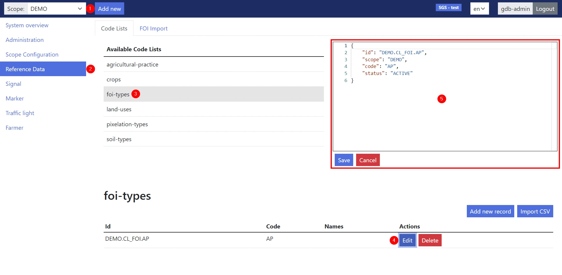
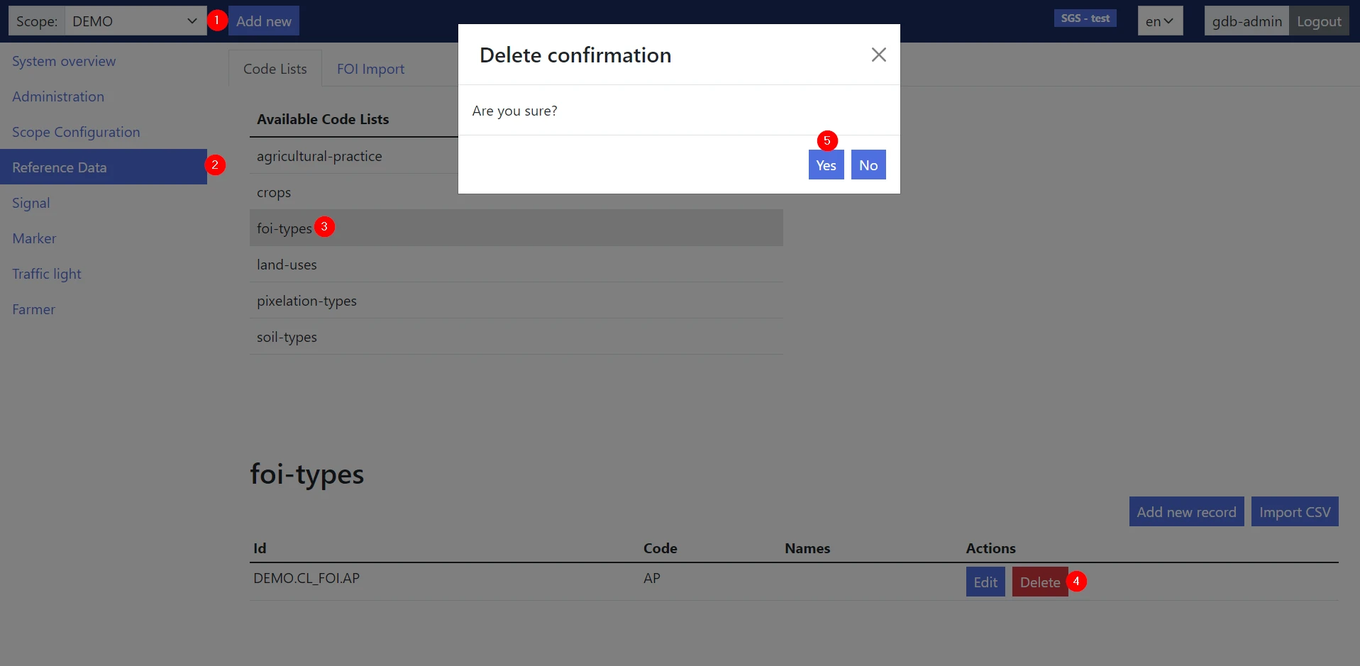
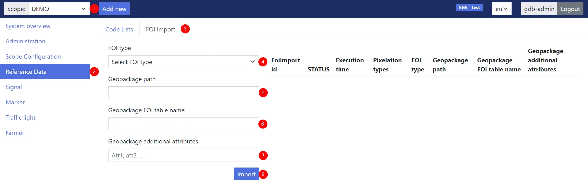
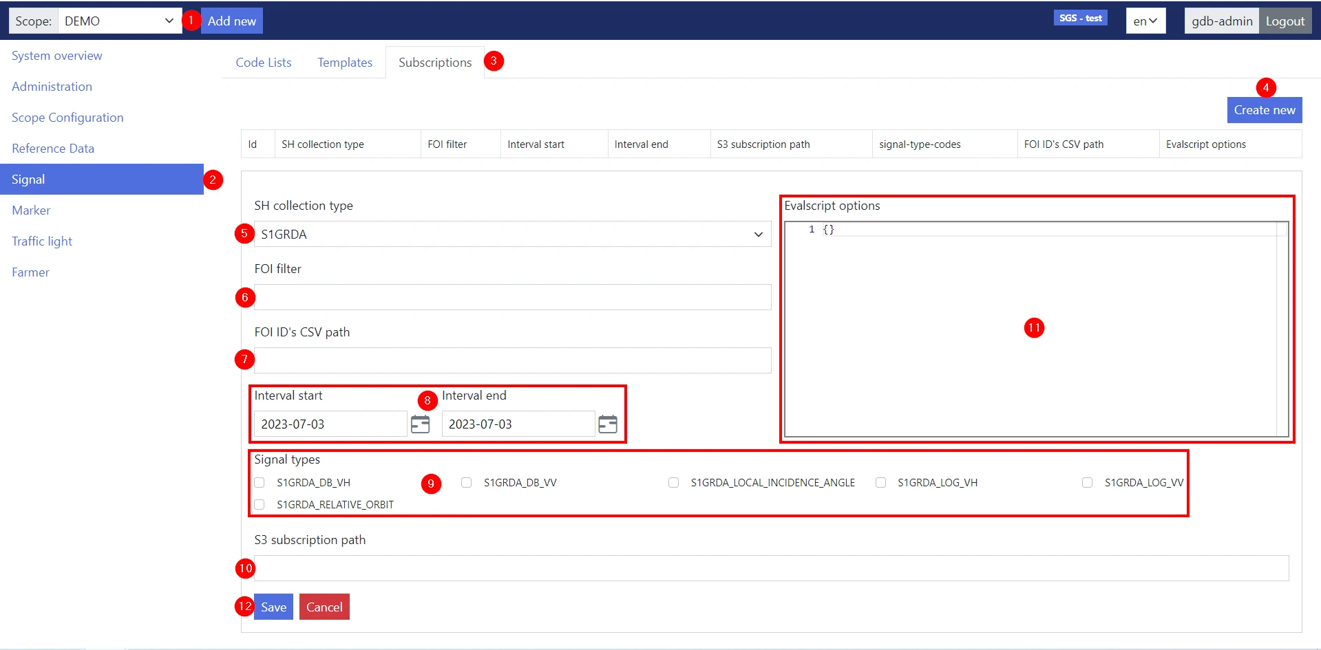
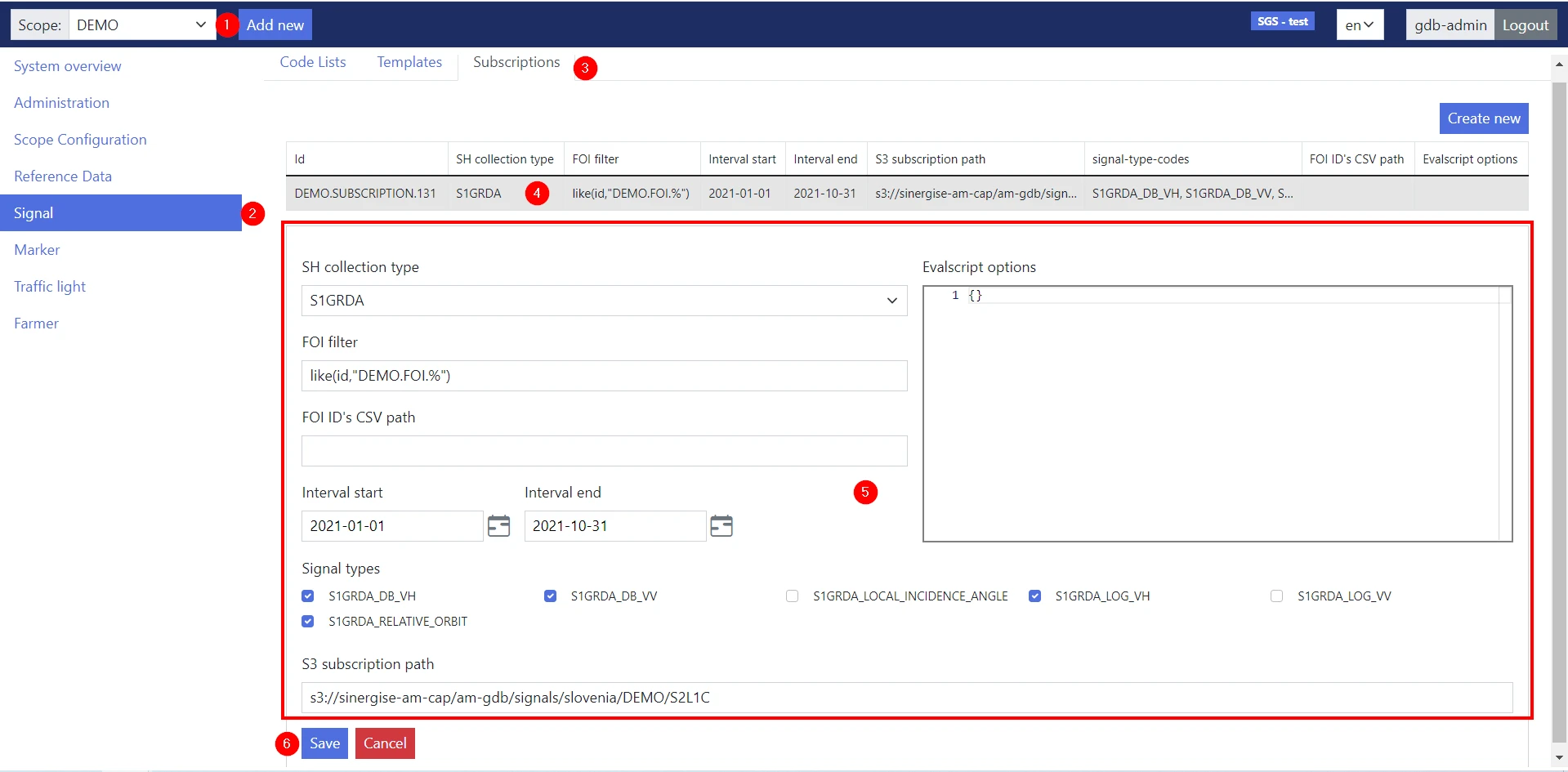
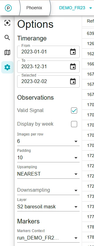
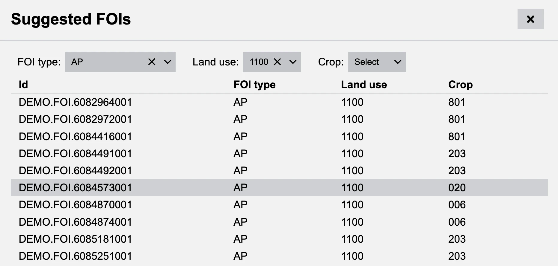
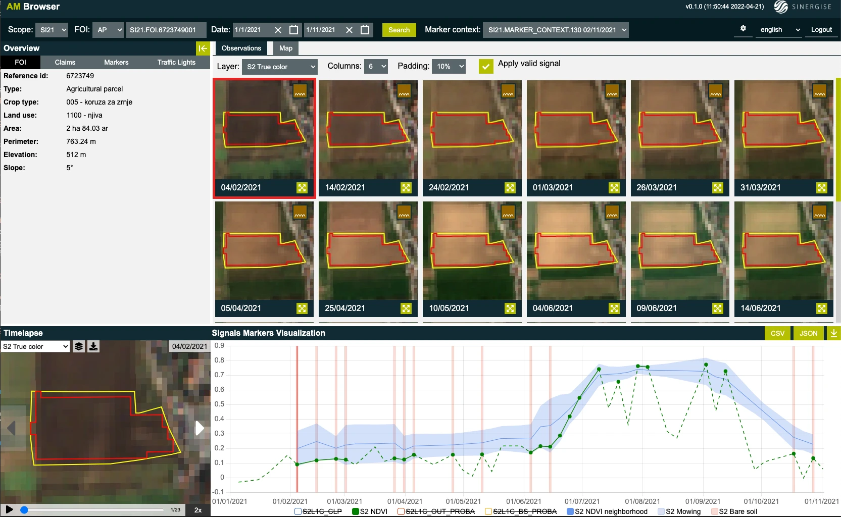
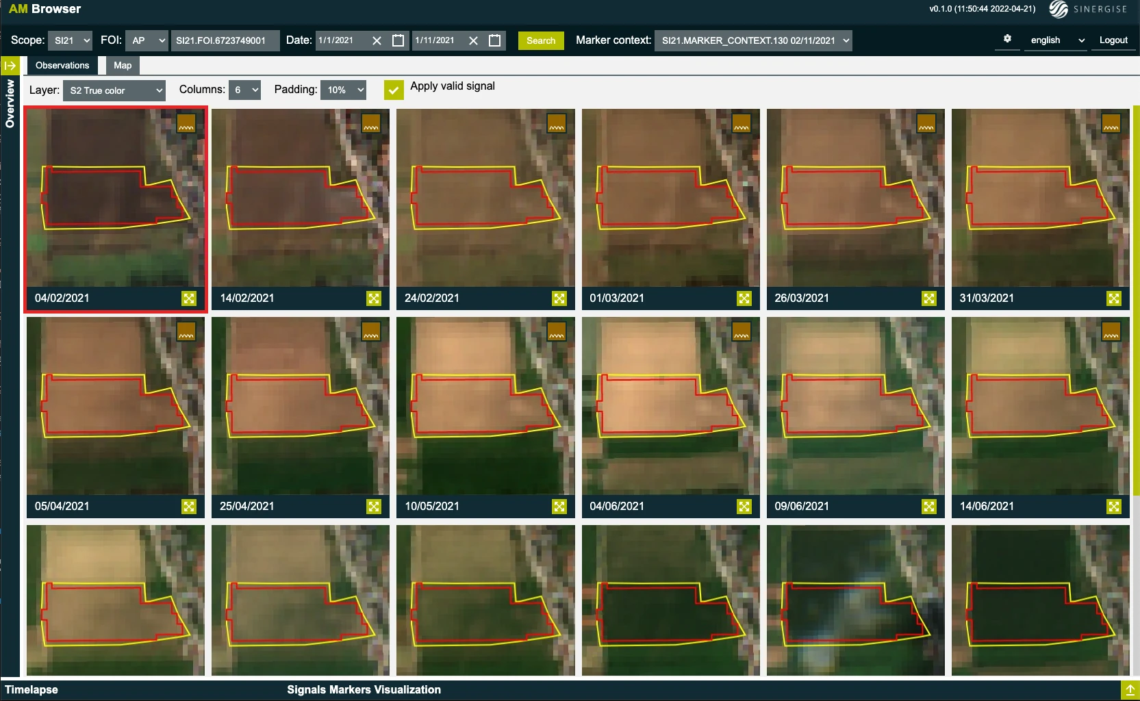
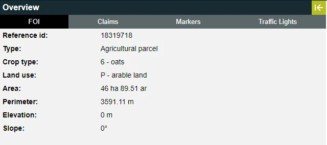
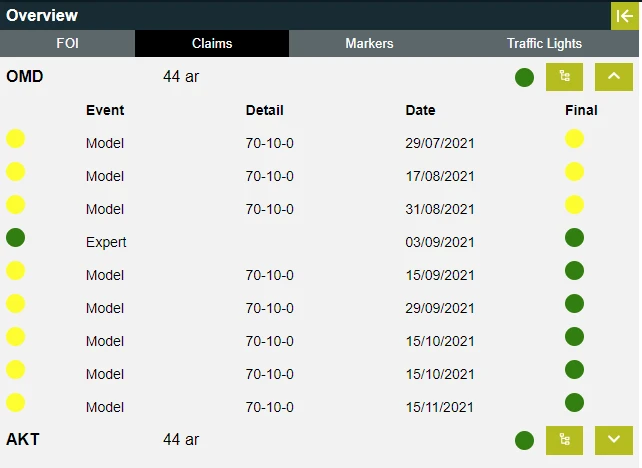
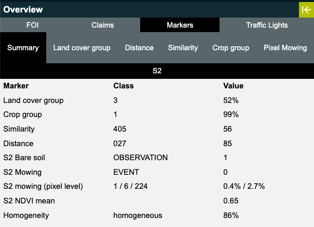
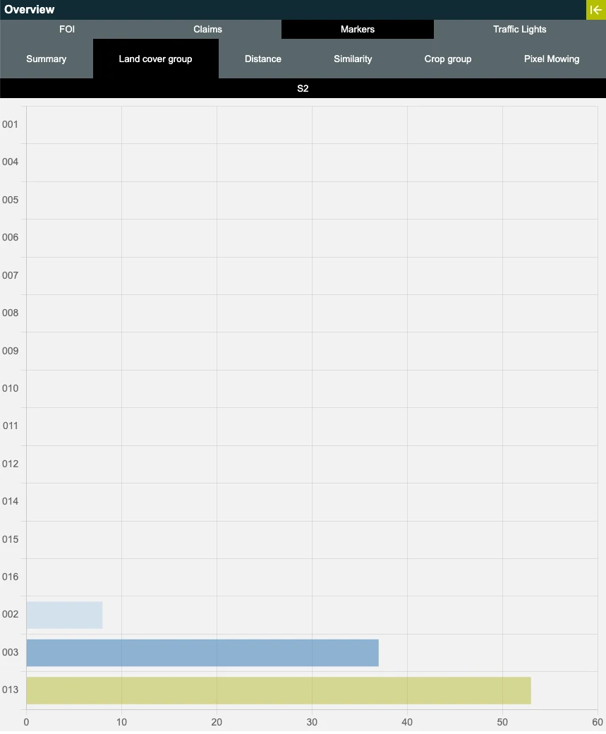
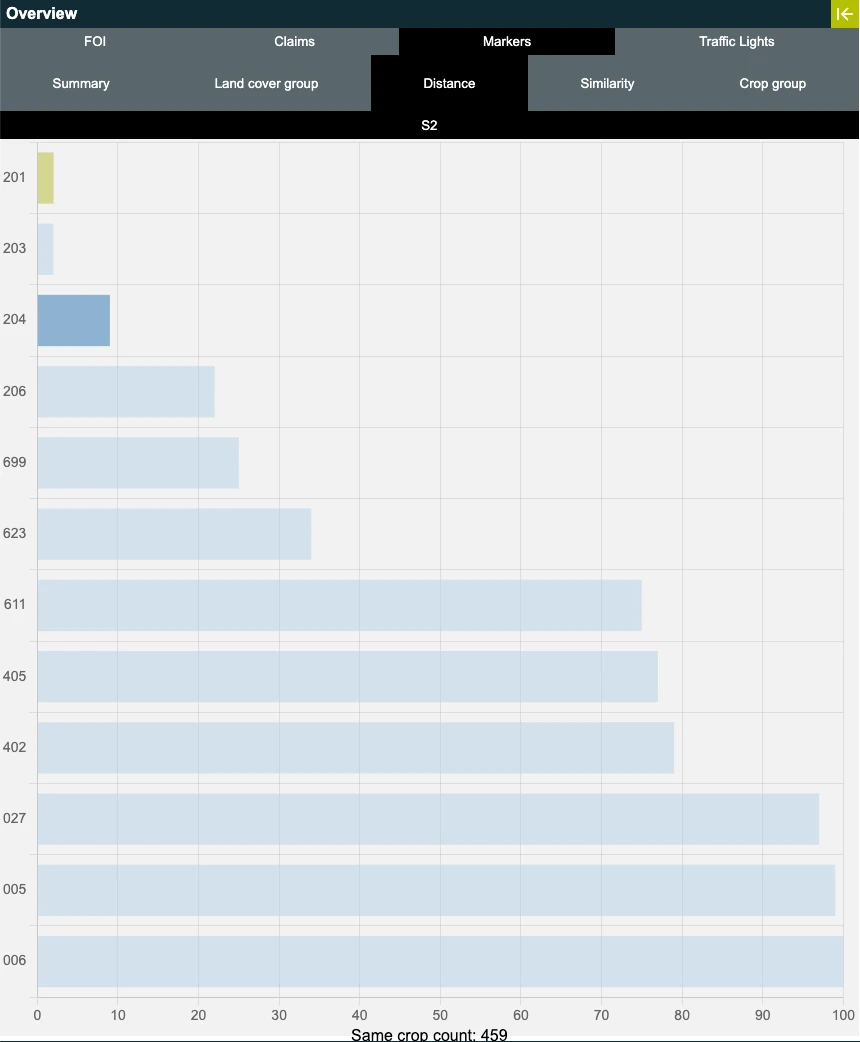
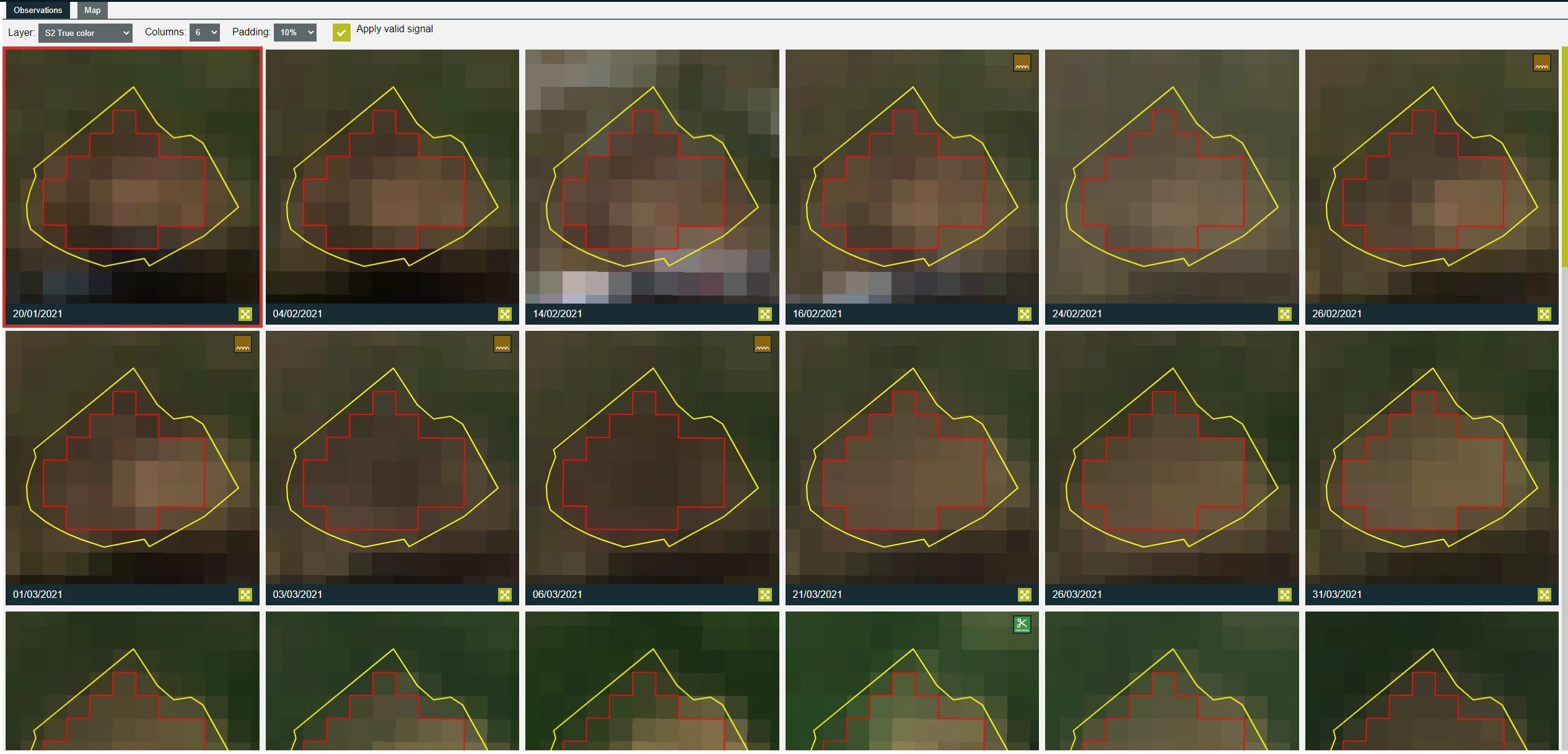

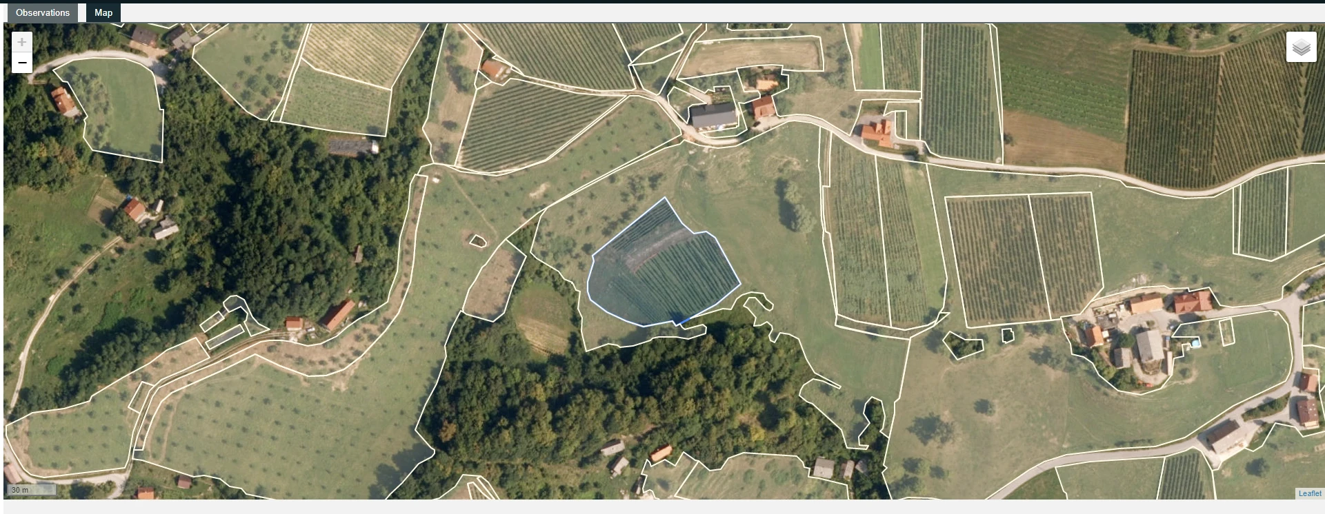

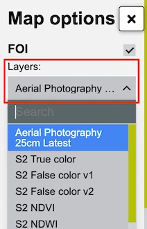
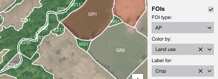
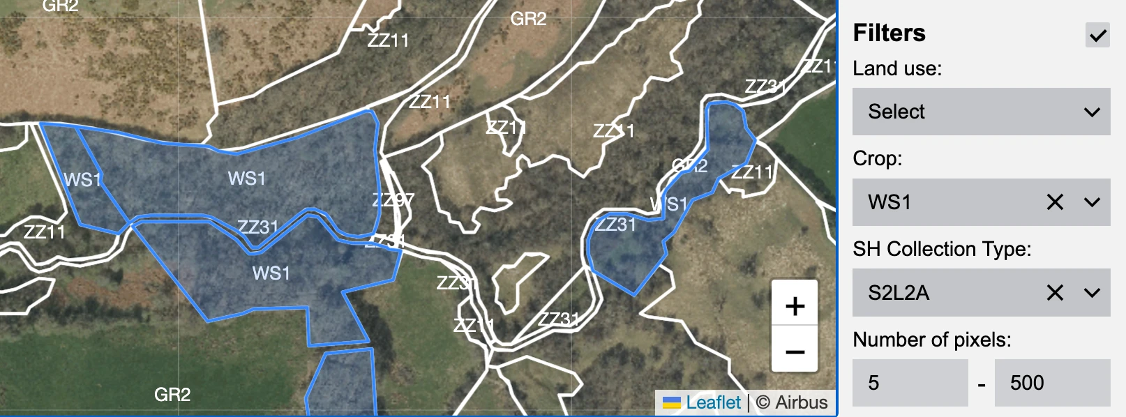
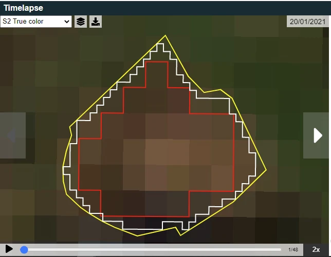
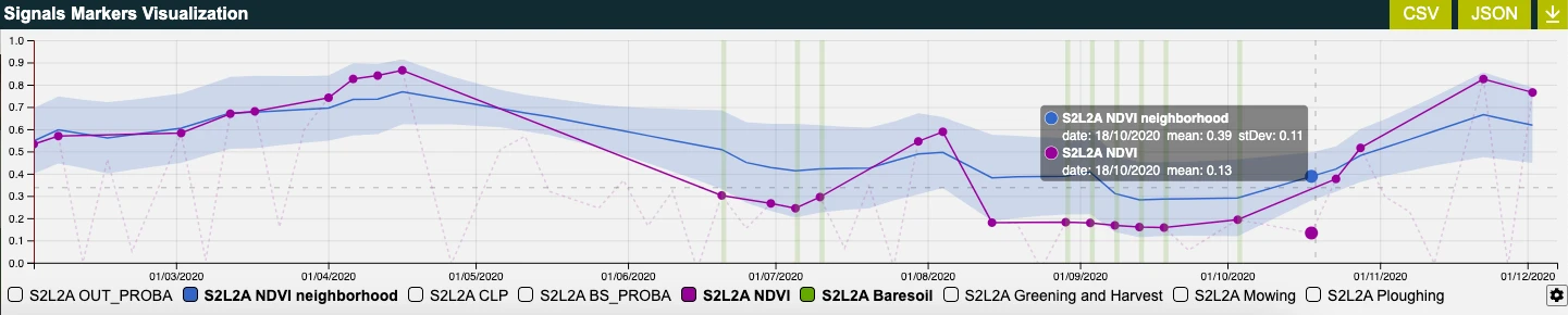
[Examples](https://docs.planet.com/data/area-monitoring/markers/bare-soil-marker/examples.md) --- Copy for LLM[View as Markdown](https://docs.planet.com/data/area-monitoring/markers/bare-soil-marker/examples/) # Bare-Soil Marker Examples ## Misclassified corn field with zero bare-soil detections ### Description FOI=[92276701](https://am-pilot.sinergise.com/phoenix/scopes/DEMO_FR23/foi-view/DEMO_FR23.FOI.92276701?from=2023-01-01\&to=2023-12-31\&selected=2023-04-17\&markerContext=DEMO_FR23.MARKER_CONTEXT.1429\&validSignal=true\&layer=ARPS-TRUE-COLOR\&displayByWeek=false\&observationsPerRow=6\&padding=10\&overlays=%5B%22FOI%22%2C%22FOIs%22%5D\&pageIndex=0\&pageSize=100) claims to grow corn, but has zero bare-soil detections, which is very atypical for corn fields as shown in the main documentation. Investigation in the Area Monitoring App reveals that corn is definitely not being cultivated on this FOI. **Key findings:** * NDVI time-series is not similar to the NDVI profile of other corn fields. * ARPS and S2 classification marker predicts vineyards group. * Similarity and distance markers suggest that buffer strip (BTA) or sunflower (TRN) are grown on this FOI. ![](/data/area-monitoring/markers/bare-soil-marker/bare-soil-marker-example1.webp) ### Link [See in Area Monitoring App](https://am-pilot.sinergise.com/phoenix/scopes/DEMO_FR23/foi-view/DEMO_FR23.FOI.92276701?from=2023-01-01\&to=2023-12-31\&selected=2023-04-17\&markerContext=DEMO_FR23.MARKER_CONTEXT.1429\&validSignal=true\&layer=ARPS-TRUE-COLOR\&displayByWeek=false\&observationsPerRow=6\&padding=10\&overlays=%5B%22FOI%22%2C%22FOIs%22%5D\&pageIndex=0\&pageSize=100) ## Grassland with presence of built-up land cover ### Description FOI=[92280460](https://am-pilot.sinergise.com/phoenix/scopes/DEMO_FR23/foi-view/DEMO_FR23.FOI.92280460?cropId=DEMO_FR23.CL_CROP.PPH\&from=2023-01-01\&to=2023-12-31\&selected=2023-07-25\&markerContext=DEMO_FR23.MARKER_CONTEXT.1429\&validSignal=true\&layer=ARPS-TRUE-COLOR\&displayByWeek=false\&observationsPerRow=6\&padding=10\&overlays=%5B%22FOI%22%2C%22FOIs%22%5D\&pageIndex=0\&pageSize=100), despite being classified as a permanent meadow, consistently shows exposed bare soil in summer observations. Further investigation in the Area Monitoring App reveals that this permanent grassland may have been partly converted to built-up land, with visible structures now present. **Key findings:** * No mowing detected. * Relatively low mean NDVI values - 0.4 with ARPS and 0.33 based on Sentinel-2 signals. ![](/data/area-monitoring/markers/bare-soil-marker/bare-soil-marker-example2.webp) ### Link [See in Area Monitoring App](https://am-pilot.sinergise.com/phoenix/scopes/DEMO_FR23/foi-view/DEMO_FR23.FOI.92280460?cropId=DEMO_FR23.CL_CROP.PPH\&from=2023-01-01\&to=2023-12-31\&selected=2023-07-25\&markerContext=DEMO_FR23.MARKER_CONTEXT.1429\&validSignal=true\&layer=ARPS-TRUE-COLOR\&displayByWeek=false\&observationsPerRow=6\&padding=10\&overlays=%5B%22FOI%22%2C%22FOIs%22%5D\&pageIndex=0\&pageSize=100) ## Winter barley ### Description FOI=[92273815](https://am-pilot.sinergise.com/phoenix/scopes/DEMO_FR23/foi-view/DEMO_FR23.FOI.92273815?from=2023-01-01\&to=2023-12-31\&selected=2023-07-25\&markerContext=DEMO_FR23.MARKER_CONTEXT.1429\&validSignal=true\&layer=ARPS-TRUE-COLOR\&displayByWeek=false\&observationsPerRow=6\&padding=10\&overlays=%5B%22FOI%22%2C%22FOIs%22%5D\&pageIndex=0\&pageSize=100) claims to grow winter barley. **Key findings:** * NDVI time-series and crop-group classification are consistent with this claim. * There are bare-soil observations only in July and during October-December. Most probably this FOI had another crop undersown, which started to grow after winter barley was harvested. The bare-soil observations in July are from the time when there was no or very little photosynthetic vegetation present on the FOI. ![](/data/area-monitoring/markers/bare-soil-marker/bare-soil-marker-example3.webp) ### Link [See in Area Monitoring App](https://am-pilot.sinergise.com/phoenix/scopes/DEMO_FR23/foi-view/DEMO_FR23.FOI.92273815?from=2023-01-01\&to=2023-12-31\&selected=2023-07-25\&markerContext=DEMO_FR23.MARKER_CONTEXT.1429\&validSignal=true\&layer=ARPS-TRUE-COLOR\&displayByWeek=false\&observationsPerRow=6\&padding=10\&overlays=%5B%22FOI%22%2C%22FOIs%22%5D\&pageIndex=0\&pageSize=100) --- Copy for LLM[View as Markdown](https://docs.planet.com/data/area-monitoring/markers/binary-land-cover-marker/) # Binary Land-Cover Marker ## Basic info Binary land-cover marker is a set of binary land-cover classifiers that are able to give insights into the land-cover of each pixel of a FOI. These are: built-up, bare-soil, forest and water land-cover binary classifiers. The combination of these binary land-cover classifiers gives us our own proprietary on-demand scene classification map that can be applied to any single Sentinel-2 observation. ## Marker output Scene classification example can be found in the image below for a medium-sized area in Savinjska valley, Slovenia. ![](/data/area-monitoring/markers/binary-land-cover-marker/binary_land_use_layers.webp) The color coding of pixels is as follows: * red color - identified as likely built-up / artificial structure * orange color - identified as likely bare-soil * green color - identified as likely forest / trees * blue color - identified as likely water ## Further info If the reader is interested in more detail about how such a binary land-cover classifier is trained, we refer him to our Medium blog-post on this topic - [Area Monitoring: How to train a binary classifier for built-up areas](https://medium.com/sentinel-hub/area-monitoring-how-to-train-a-binary-classifier-for-built-up-areas-7f2d7114ed1c). This blog-post focuses on training and evaluating the built-up binary land-cover classifier, however the procedures and findings therein can be translated to other classifiers also. All of these pixel-wise predictions are available also in the Browser-App to help understand the land-cover of specific FOIs. You can view them by choosing them in the drop-down just above the image chips: ![](/data/area-monitoring/markers/binary-land-cover-marker/layer-dropdown.webp) As an example, the layer based on the forest classifier probability is shown. You can also choose the layer in the same way in the Timelapse window in the bottom left. The outputs of these models are also available in the produced signal datasets we use to calculate other markers and can be used to find FOIs where we suspect that the claimed and actual land-covers differ substantially. One option is to calculate the temporal average of one of these signals for a multi-month period. FOIs with even small portions of built-up pixels can stand-out in this approach, since they have a higher average than FOIs without built-up pixels. ## Links [Blog post](https://medium.com/sentinel-hub/area-monitoring-how-to-train-a-binary-classifier-for-built-up-areas-7f2d7114ed1c) about Identifying built-up areas
[Examples](https://docs.planet.com/data/area-monitoring/markers/binary-land-cover-marker/examples.md) --- Copy for LLM[View as Markdown](https://docs.planet.com/data/area-monitoring/markers/binary-land-cover-marker/examples/) # Binary Land-Cover Marker Examples ## Agricultural field with built-up structures ### Description The first example, FOI = [92287319](https://am-pilot.sinergise.com/phoenix/scopes/DEMO_FR23/foi-view/DEMO_FR23.FOI.92287319?from=2023-01-01\&to=2023-12-31\&selected=2023-03-01\&markerContext=DEMO_FR23.MARKER_CONTEXT.1429\&upsampling=NEAREST\&validSignal=true\&layer=SENTINEL2-BUILD-UP-MASK\&displayByWeek=false\&observationsPerRow=6\&padding=10\&baseLayer=Satellite\&overlays=%5B%22FOI%22%2C%22FOIs%22%5D\&pageIndex=0\&pageSize=100\&key=NEAREST), is claimed to be an agricultural area. However, using the binary land-cover marker approach outlined above, we have found that part of the FOI is likely covered with artificial surfaces. **Key findings:** * The built-up mask (applied to Sentinel-2) clearly shows artificial structures within the agricultural area * This finding is confirmed by the timelapse component in the bottom right corner of the screen * External validation through [Roads and building detection](https://www.planet.com/pulse/mapping-all-of-earths-roads-and-buildings-from-space/) corroborates the presence of built-up structures ![](/data/area-monitoring/markers/binary-land-cover-marker/binary_marker_example.webp) ### Link [See in Area Monitoring App](https://am-pilot.sinergise.com/phoenix/scopes/DEMO_FR23/foi-view/DEMO_FR23.FOI.92287319?from=2023-01-01\&to=2023-12-31\&selected=2023-03-01\&markerContext=DEMO_FR23.MARKER_CONTEXT.1429\&upsampling=NEAREST\&validSignal=true\&layer=SENTINEL2-BUILD-UP-MASK\&displayByWeek=false\&observationsPerRow=6\&padding=10\&baseLayer=Satellite\&overlays=%5B%22FOI%22%2C%22FOIs%22%5D\&pageIndex=0\&pageSize=100\&key=NEAREST) ## Artificial surface with consistently low NDVI ### Description The second example, FOI = [92288632](https://am-pilot.sinergise.com/phoenix/scopes/DEMO_FR23/foi-view/DEMO_FR23.FOI.92288632?from=2023-01-01\&to=2023-12-31\&selected=2023-09-06\&markerContext=DEMO_FR23.MARKER_CONTEXT.1429\&upsampling=NEAREST\&validSignal=true\&layer=SENTINEL2-BARESOIL-MASK\&displayByWeek=false\&observationsPerRow=6\&padding=10\&baseLayer=Satellite\&overlays=%5B%22FOI%22%2C%22FOIs%22%5D\&pageIndex=0\&pageSize=100), is also claimed to be arable land. However, we can clearly see from the example that the FOI is inconsistent with this claim due to consistently low NDVI values throughout the year. **Key findings:** * Constantly low NDVI values indicate absence of healthy vegetation * The temporal pattern is inconsistent with typical agricultural land use * Visual inspection confirms the presence of artificial surfaces rather than agricultural activity ![](/data/area-monitoring/markers/binary-land-cover-marker/inconsistent_pixels.webp) ### Link [See in Area Monitoring App](https://am-pilot.sinergise.com/phoenix/scopes/DEMO_FR23/foi-view/DEMO_FR23.FOI.92288632?from=2023-01-01\&to=2023-12-31\&selected=2023-09-06\&markerContext=DEMO_FR23.MARKER_CONTEXT.1429\&upsampling=NEAREST\&validSignal=true\&layer=SENTINEL2-BARESOIL-MASK\&displayByWeek=false\&observationsPerRow=6\&padding=10\&baseLayer=Satellite\&overlays=%5B%22FOI%22%2C%22FOIs%22%5D\&pageIndex=0\&pageSize=100) --- Copy for LLM[View as Markdown](https://docs.planet.com/data/area-monitoring/markers/crop-and-land-use-markers/) # Crop and Land-Use Markers ## Basic info The crop- and land-group markers can be used to determine consistency of a agricultural parcel (FOI) with its declared crop and land-use. Both markers use the same architecture, so we will describe the inner workings of both on the example of the **crop-group** marker. ## Further info ### Crop-group marker Each FOI has a declared crop. The crop defines the behavior of the time-series of signals throughout the year. As an example, below we show the NDVI time-series of two FOIs. The one in blue has an associated crop with ID 005 (corn), while the one in orange has an associated crop with ID 204 (grass). ![](/data/area-monitoring/markers/crop-and-land-use-markers/corn-vs-meadow.webp) Clearly, both crops have vastly different behavior and should thus be easily recognizable. However, not all crops are as easily separable. Next we show two FOIs with declared winter wheat (blue) and winter barley (orange). ![](/data/area-monitoring/markers/crop-and-land-use-markers/winter-wheat-vs-barley.webp) We can see that, ignoring the secondary crop sown after July, the two crops are pretty much inseparable. There are many such **crop groups** which are difficult to recognize them as separate with remote sensing. For instance winter grains that we show above, grass and grass-like annual crops like alfalfa, summer grains and many more. To achieve more accurate and reliable results, we often take advantage of these natural groupings and treat all crops inside the group as one training/prediction class, however this is not strictly necessary. We could treat each crop as a separate class in hopes of gaining the ability to intra-separate crops in groups, however this usually comes at a relatively drastic cost of performance, especially in confusion of crops within the same group. In Slovenia, there is approximately 200 crops grouped into 31 crop groups. Some of the more populous ones are grasses, winter grains and summer grains. ### Training of the model The model that we train on the crop-group classes is a Long short-term memory (LSTM) model \[[1](https://arxiv.org/abs/1905.11893), [2](https://arxiv.org/abs/1910.10536)], which is based on the recurrent neural network architecture. This architecture is especially tailored to be able to recognize classes from patterns in time-series like satellite data. The training data is always based on the desired year agricultural parcel reference data (declarations), however it is possible to include historical data if the reference data is made available. This helps boost the numbers of underrepresented classes, increasing the accuracy of recognizing classes which are rare in a specific year. Since we use declaration reference data as our target classes, we need to make sure, to have the declarations as reliable as possible, since it is possible that declarations are incorrect. To clean some of the incorrect declaration noise out of the training data we use other markers, if they indicate a discrepancy between the claim and the real state. To be more concrete, we filter the FOIs based on: * the outliers from the distance marker. As an example we show a FOI that has been declared as a meadow (204), however the distance and similarity markers point to this claim to likely be incorrect. ![](/data/area-monitoring/markers/crop-and-land-use-markers/distance.webp) * the homogeneity marker, since it points-out FOIs that are likely heterogeneous and could thus confuse the model. An example of a FOI that apparently has several crops growing at the same time is shown below. ![](/data/area-monitoring/markers/crop-and-land-use-markers/homogeneity.webp) After the likely incorrect claims are filtered, the marker randomly divides all available FOIs into five folds: A, B, C, D and E. For each of these folds, a separate model is trained on the rest of the folds, after which a prediction is made on the specific fold that is left-out. As an example, when predicting on FOIs from fold A, we use the model trained on folds B-E and equivalent for other left-out folds. In this way, we can get predictions with models that have not seen a FOI during training for all FOIs in our dataset. ### Land-group marker The basic building blocks of the land-group marker are exactly the same as for the crop-group marker. The only difference is that the declared land-use labels are grouped into land-groups instead of crops and used as training and prediction classes. Alongside agricultural land-uses, we also include non-agricultural ones to augment our training classes. The most prominent and interesting are forests and built-up land-uses. | Built-up | Forests | | --------------------------------------------------------------------------- | ------------------------------------------------------------------------- | | ![](/data/area-monitoring/markers/crop-and-land-use-markers/buildings.webp) | ![](/data/area-monitoring/markers/crop-and-land-use-markers/forests.webp) | By including these non-agricultural land-uses we can hopefully be able to recognize them if an agricultural parcels land-use has transformed into an non-agricultural ones. ## Links [Blog post](https://medium.com/sentinel-hub/area-monitoring-crop-type-marker-1e70f672bf44) about Crop Type marker
[Examples](https://docs.planet.com/data/area-monitoring/markers/crop-and-land-use-markers/examples.md) --- Copy for LLM[View as Markdown](https://docs.planet.com/data/area-monitoring/markers/crop-and-land-use-markers/examples/) # Crop and Land-Use Marker Examples ## High confidence in crop group prediction ### Description The first example, FOI = [92278988](https://am-pilot.sinergise.com/phoenix/scopes/DEMO_FR23/foi-view/DEMO_FR23.FOI.92278988?from=2023-01-01\&to=2023-12-31\&selected=2023-10-03\&markerContext=DEMO_FR23.MARKER_CONTEXT.1429\&upsampling=NEAREST\&validSignal=true\&layer=ARPS-NDVI\&displayByWeek=false\&observationsPerRow=6\&padding=10\&overlays=%5B%22FOI%22%2C%22FOIs%22%5D\&pageIndex=0\&pageSize=100), is declared as wine (vineyard crop group). The classification marker unequivocally agrees with this declaration, showing 100% confidence that the FOI belongs to the vineyards crop group. **Key findings:** * Perfect match between declared crop type and predicted crop group * 100% pseudo-probability score indicates very high model confidence * Visual inspection confirms vineyard characteristics ![](/data/area-monitoring/markers/crop-and-land-use-markers/crop_group_marker1.webp) ### Link [See in Area Monitoring App](https://am-pilot.sinergise.com/phoenix/scopes/DEMO_FR23/foi-view/DEMO_FR23.FOI.92278988?from=2023-01-01\&to=2023-12-31\&selected=2023-10-03\&markerContext=DEMO_FR23.MARKER_CONTEXT.1429\&upsampling=NEAREST\&validSignal=true\&layer=ARPS-NDVI\&displayByWeek=false\&observationsPerRow=6\&padding=10\&overlays=%5B%22FOI%22%2C%22FOIs%22%5D\&pageIndex=0\&pageSize=100) ## Lower confidence in crop group prediction ### Description The next example is FOI = [92269936](https://am-pilot.sinergise.com/phoenix/scopes/DEMO_FR23/foi-view/DEMO_FR23.FOI.92269936?cropId=DEMO_FR23.CL_CROP.MIS\&from=2023-01-01\&to=2023-12-31\&selected=2023-04-05\&markerContext=DEMO_FR23.MARKER_CONTEXT.1429\&upsampling=NEAREST\&validSignal=true\&layer=ARPS-NDVI\&displayByWeek=false\&observationsPerRow=6\&padding=10\&overlays=%5B%22FOI%22%2C%22FOIs%22%5D\&pageIndex=0\&pageSize=100), which is claimed to be corn, belonging to the corn grain and silage (2) crop group. The crop-group marker shows mixed results: **ARPS crop group classification:** * Predicts "other oilseeds" with 80% confidence **Sentinel-2 crop group classification:** * Predicts "corn grain and silage" with 51% confidence (relatively low) * Alternative prediction: "other oilseeds" with 44% confidence **Technical interpretation:** Upon visual inspection, the claim appears correct. The presence of winter crop until late March likely postponed the corn greening period, which may have affected the classification. This example demonstrates the marker's confusion between very similar crops. The confusion between corn and oilseed crops can be attributed to both crop types having high NDVI values during summer, making the classes distinguishable but not trivially separable. Despite the mixed signals, both markers still suggest the claim is reasonable. ![](/data/area-monitoring/markers/crop-and-land-use-markers/crop_group_marker2.webp) ### Link [See in Area Monitoring App](https://am-pilot.sinergise.com/phoenix/scopes/DEMO_FR23/foi-view/DEMO_FR23.FOI.92269936?cropId=DEMO_FR23.CL_CROP.MIS\&from=2023-01-01\&to=2023-12-31\&selected=2023-04-05\&markerContext=DEMO_FR23.MARKER_CONTEXT.1429\&upsampling=NEAREST\&validSignal=true\&layer=ARPS-NDVI\&displayByWeek=false\&observationsPerRow=6\&padding=10\&overlays=%5B%22FOI%22%2C%22FOIs%22%5D\&pageIndex=0\&pageSize=100) --- Copy for LLM[View as Markdown](https://docs.planet.com/data/area-monitoring/markers/field-delineation/) # Field Delineation ## Basic info The field delineation marker produces boundaries of the agricultural parcels by clustering the agricultural pixels according to spatial, spectral and temporal properties. The delineated boundaries can aid the farmers speed up the declaration process and the paying agencies to better monitor changes in agricultural use. | Sentinel-2 | Field delineations | | ------------------------------------------------------------------------------ | ------------------------------------------------------------------------------ | | ![](/data/area-monitoring/markers/field-delineation/examples-2017-s2-001.webp) | ![](/data/area-monitoring/markers/field-delineation/examples-2017-fd-001.webp) | The marker automatically outputs polygon vectors defining agricultural parcels based on Sentinel-2 imagery, although the marker can be seamlessly adapted to work with any remote sensing imagery as an input. The marker was developed as part of the NIVA H2020 project, and thus far has been used for generating parcels for paying agencies, insurance companies and research centres for several regions in Europe and North America. The marker uses state-of-the-art deep learning (DL) algorithms. The codebase is available in a [GitHub repository](https://github.com/sentinel-hub/field-delineation), and a demo version is available on the [Euro Data Cube](https://collections.eurodatacube.com/field-delineation/). ## Further info The marker can be fine-tuned to the users' needs, for instance using existing GSAA datasets to train a deep learning model, or can be used as an off-the-shell algorithm using a deep learning model pre-trained on a different AOI. The marker can estimate parcel boundaries for each cloudless pixel in a Sentinel-2 imagery, and the user can select the time interval over which estimates are aggregated. This approach allows to monitor changes in parcel boundaries, which reflect agricultural activity during the growing season. In a nutshell, the following steps to produce boundaries of the agricultural parcels are performed: * split the AOI into a regular grid to speed up processing through massive parallelization * download remote sensing imagery for the time period of interest * *(optional)* if GSAA data is available, train and evaluate the DL model on reference GSAA and remote sensing imagery * predict and post-process agricultural parcel boundaries on remote sensing imagery for the time period of interest *In case the reference labels are not available, we can also skip step 3 and employ a pre-trained network on data from a different AOI.* ### Splitting AOI into a grid The AOI is split into a regular grid. Each cell, for example, EOPatch, of the grid has size as we find appropriate, and overlaps with the neighbouring cell a given amount of pixels. Splitting into cells allows to massively parallelize the processing, and the overlap ensures that the results are merged seamlessly. On the image below: Ukraine split into tiles of 10km x 10km, tiles are in their own UTM zone. ![](/data/area-monitoring/markers/field-delineation/ua-split.webp) ### Data download For the selected time periods, remote sensing images are downloaded for each EOPatch as well as the cloud masks. Data downloading is executed using Sentinel Hub Batch Processing API. ### Analysis of cloud and snow coverage Once the remote sensing imagery and cloud masks are available for each EOPatch, statistics over the available months are computed to estimate how many cloudless scenes are available. Our field delineation algorithm produces estimates for each available acquisition, however, only fields estimated for acquisitions with cloud and snow coverage below 5% of area of the EOPatch are typically kept and a consensus generated. This is performed in order to ensure that clouds and other artifacts do not affect the estimation of boundaries. On the image below: invalid observations over a month. ![](/data/area-monitoring/markers/field-delineation/invalid-eopatches-2022-06.webp) ### Reference data and sampling (optional) GSAA vectors are a great reference data for training of the ML model: for a given year, the majority of the GSAA parcels correctly match the agricultural land cover, with the exception of a minority of incorrect parcels resulting from outdated information or incorrect applications. If available, these vectors can be used to fine-tune the marker to improve its parcel boundary estimation. The GSAA along with the remote sensing imagery is further sampled into smaller patchlets to speed up the training of the deep learning model. Using sampling, a constraint can be made on the minimal area covered by the reference GSAA in each sample, allowing to control the amount of positive and negative examples the model sees. ### Normalization As we want our model to perform well over timestamps taken over the whole year, it is very important how the data is normalized. For each individual patchlet timestamp, statistics that could be used for normalization are calculated for each band. As well as computing overall statistics, we evaluate these temporally to establish whether a single or multiple normalization factors for the time period of interest are needed. We look at mean, standard deviation and quantiles for each month. As mentioned above, in case the reference labels are not available to fine-tune our deep learning algorithm, we use an existing model trained on data in another AOI. In this case, a key factor to achieve meaningful results is to adequately normalize the input reflectance values, so that the input distributions for the area of interest (where the boundaries are predicted) are as aligned as possible to the reflectance distributions the model has seen during training. ### Semantic segmentation We apply semantic segmentation on each single-scene separately, and combine predictions temporally at a later stage. A model trained this way should learn to be invariant to the time-period of interest. The aim of the parcel delineation in CAP practices is generally to monitor agricultural land cover throughout the growing season, but the beginning of the season is of particular interest as is typically the time the farmers fill in their applications. A model that can generalise to different time periods seems therefore useful in this perspective, and that justifies our choice of training a single-scene model and combining temporally the predictions in a second stage. ### Temporal merging Once the model estimates field boundaries, for example, extent and boundary masks, for each timestamp for each EOPatch, these are temporally and spatially merged to derive a single probability map, which is then contoured to obtain the final vector polygons. The temporal merging generates a consensus of extent and boundary masks over a given time period (see example on figure below). ![](/data/area-monitoring/markers/field-delineation/36UWU_6_0-prediction.webp) ### Contouring The consensus raster extent and boundary masks for the chosen time period are spatially merged and contoured to derive enclosed vector polygons. Parameters for the contouring can be optimised to control the appearance of the final polygons. ### Shape attributes For each estimated polygon, we compute its area, circumference, shapeness and circumference/area (CA) ratio. Shapeness calculates the Hausdorff distance between the polygon and its minimum rotated rectangle, while the CA ratio provides an indication of the regularity of the polygon. These attributes can be used to further filter out polygons which are likely not cultivated, for example, with large areas and large values of shapeness (see some examples in the figure below). ![](/data/area-monitoring/markers/field-delineation/shapeness-example.webp) ### Dynamic analysis The field delineation marker can be computed for different time periods, and the resulting polygons can be used to track and monitor agricultural activity. For instance, estimated parcels derived early in the season can be compared to parcels estimated at peak growing season, providing insights into whether the field boundaries changed or not. The figures below show such a comparison, and the quantitative metrics that quantify changes in field contours, that can be further used to monitor agricultural activity. ![](/data/area-monitoring/markers/field-delineation/ps_field-comparison-MAR-JUL_1.webp) ![](/data/area-monitoring/markers/field-delineation/ps_field-comparison-MAR-JUL_2.webp) The quantitative metrics can be computed for each estimated field, and used to derive overall insights into the performance of the marker, as well as into the changes due agricultural activity, as shown below. These plots show that parcels tend to change more at the beginning and end of the growing season, for example, from March to May and from August to October, due to ploughing and harvesting activities which can reduce the visibility of boundaries. Estimated parcels show less changes and are possibly more accurate at the peak of the growing season, for example, from May to July. | | | | ------------------------------------------------------------------------------------ | ------------------------------------------------------------------------------ | | ![](/data/area-monitoring/markers/field-delineation/s2_MAY-JUN_JUL-AUG-scatter.webp) | ![](/data/area-monitoring/markers/field-delineation/s2_quadrant_analysis.webp) | ## Links [Webinar](https://www.youtube.com/watch?v=czRCApJCYIo): Automated Agricultural Field Delineation Tool
[Blog post](https://medium.com/sentinel-hub/parcel-boundary-detection-for-cap-2a316a77d2f6) about Parcel boundary detection for CAP
[Interactive interface](http://parcelio.sentinel-hub.com/) for viewing delineated fields in Lithuania for June 2020 --- Copy for LLM[View as Markdown](https://docs.planet.com/data/area-monitoring/markers/greening-harvest-marker/) # Greening and Harvest Marker ## Basic info The greening and harvest marker identifies greening and harvest phases in the FOI's NDVI time series and combines them into a single period that signifies the life cycle of a crop. It can be a very useful tool for detecting presence of **catch crops** or **green cover** and **nitrogen-fixing crops**, for example, the management practices under the [EFA obligation](https://eur-lex.europa.eu/legal-content/EN/ALL/?uri=COM%3A2017%3A152%3AFIN) of which the main objective is to safeguard and improve biodiversity on farms. The greening and harvest marker can give answers to the following questions: * When was the main crop sown and when harvested? * After the harvest of the main crop, when did the second crop start developing? * Until when was the second crop present on the field, for example, when was it harvested? If greening and harvest marker is fused with bare-soil marker results, then the combined results can provide answers to questions like: * How was the soil prepared before sowing of the main crop - was the field ploughed or not? * Was the second crop established with undersowing? * Before sowing of the second crop, was the field ploughed or did the farmer use some light cultivation techniques? Was the stubble left in the field after the harvest of the main crop? The greening phase starts when the crop emerges from the soil (NDVI value is low) and ends when it fully matures (NDVI will reach a plateau). In between, NDVI values will steadily increase. When crop is harvested, plants are partially or entirely removed from the field. This activity is reflected in a sudden drop of NDVI value, often (but not necessarily) followed by a period when bare soil is detected. Harvest phase typically does not last long. Its detection is triggered by an abrupt and significant drop of the NDVI value. The greening and harvest marker output can be visually presented with a plot, for example, like below for FOI, where we observe 2 greening periods and one harvest period in between. ![](/data/area-monitoring/markers/greening-harvest-marker/GH-marker-plot.webp) The greening and harvest marker is a means to identify changes in the NDVI time series that indicate agricultural activity on a FOI. The greening/harvest phase reflects the duration of the change in the NDVI time series and therefore the period within which we expect the activity to have taken place. * Light green strip corresponds to an extended greening phase, dark green strip to the "actual" greening phase. * Similarly, light red strip corresponds to an extended harvest phase and dark red strip to the "actual" harvest phase. The distinction between the extended and "actual" phase becomes important when we condition the eligibility with, for example, the start of the greening phase or harvesting of the crop within a required or forbidden period. If we take a look at the harvest period and imagine a potential rule that the main crop should not be harvested before June 15th: the "actual" harvest period starts when we, for the first time, notice the consequence of the harvest, for example, a significant drop of the NDVI value, and this happened after June 15th. If we were validating the eligibility based on the start of the extended harvest phase, FOI would be found harvested before the June 15th and therefore ineligible. * Observation marks enclosed in red diamonds indicate when bare soil was detected. We can, for example, mathematically describe a requirement for presence of baresoil observations before the greening or after the harvest phase, within a specified number of days. For undersown crops, the bare-soil before the greening phase is not required. However, for some practices, for example, for non-winter crops sown after the main crop, bare-soil might be mandatory. * Black arrow indicates the total duration of one greening-harvest cycle. The changes in vegetation cover are best visible in the Sentinel-2 False colour time series visualisation. In the image below, the green stripe on top of the images marks the greening phase, where we can observe the intensifying of the red colour within the FOI's boundary, indicating vegetation growth. After the vegetation reaches full maturity (and the NDVI value plateaus), we can observe the beginning of the harvest phase (marked with the yellow strip) as the intensity of the red false colour starts fading towards a more brownish colour, indicating the underlying soil, exposed after the vegetation removal. We can also see that towards the end of the harvest period, there are observations of exposed bare soil (marked with the brown icon). After harvest, we observe a new greening phase as the vegetation picks up again in late summer/early autumn. ![](/data/area-monitoring/markers/greening-harvest-marker/S2_FC_marked.webp) ## Marker output In the [Area Monitoring App](https://docs.planet.com/data/area-monitoring/applications/area-monitoring-browser.md), the greening and harvest periods are marked with reddish stripes in the `Signals Markers Visualization` component at the bottom. The green stripe marks the greening phase and the red one indicates the harvest phase. See example FOI = [92273921](https://am-pilot.sinergise.com/phoenix/scopes/DEMO_FR23/foi-view/DEMO_FR23.FOI.92273921?refId=\&cropId=DEMO_FR23.CL_CROP.MID\&from=2023-01-01\&to=2023-12-31\&selected=2023-07-15\&markerContext=DEMO_FR23.MARKER_CONTEXT.1429\&validSignal=true\&layer=ARPS-NDVI\&displayByWeek=false\&observationsPerRow=6\&padding=10\&baseLayer=Satellite\&overlays=%5B%22FOI%22%2C%22FOIs%22%5D\&pageIndex=0\&pageSize=100) ![](/data/area-monitoring/markers/greening-harvest-marker/GH-screenshot.webp) ## Further info For a detailed description of the greening and harvest marker output, check the [Marker Service API documentation](https://docs.planet.com/data/area-monitoring/marker-service-api.md#greening-harvest-marker). ## Links [Examples](https://docs.planet.com/data/area-monitoring/markers/greening-harvest-marker/examples.md) --- Copy for LLM[View as Markdown](https://docs.planet.com/data/area-monitoring/markers/greening-harvest-marker/examples/) # Greening and Harvest Marker Examples ## Bare soil between harvest of the main crop and second crop ### Description FOI = [92274649](https://am-pilot.sinergise.com/phoenix/scopes/DEMO_FR23/foi-view/DEMO_FR23.FOI.92274649?refId=\&cropId=DEMO_FR23.CL_CROP.ORP\&from=2023-01-01\&to=2023-12-31\&selected=2023-05-13\&markerContext=DEMO_FR23.MARKER_CONTEXT.1429\&validSignal=true\&layer=ARPS-NDVI\&displayByWeek=false\&observationsPerRow=6\&padding=10\&baseLayer=Satellite\&overlays=%5B%22FOI%22%2C%22FOIs%22%5D\&pageIndex=0\&pageSize=100) had a spring barley (*Hordeum vulgare L.*) claim for the main crop. This NDVI time series indicates development of the main crop early in spring and harvest in mid-summer (see Area Monitoring App screenshot below). **Key observations:** * Greening phase detected early in spring * Harvest detected in mid-summer as expected for spring barley * Bare soil detected after harvest (marked with vertical brown lines in Signal component) * Bare soil indicates agricultural practices that removed vegetation and exposed soil, such as ploughing ![](/data/area-monitoring/markers/greening-harvest-marker/GH-92274649-AM.webp) ### Link [See in Area Monitoring App](https://am-pilot.sinergise.com/phoenix/scopes/DEMO_FR23/foi-view/DEMO_FR23.FOI.92274649?refId=\&cropId=DEMO_FR23.CL_CROP.ORP\&from=2023-01-01\&to=2023-12-31\&selected=2023-05-13\&markerContext=DEMO_FR23.MARKER_CONTEXT.1429\&validSignal=true\&layer=ARPS-NDVI\&displayByWeek=false\&observationsPerRow=6\&padding=10\&baseLayer=Satellite\&overlays=%5B%22FOI%22%2C%22FOIs%22%5D\&pageIndex=0\&pageSize=100) ## Continuous vegetation cover indicating undersown second crop ### Description FOI = [92276226](https://am-pilot.sinergise.com/phoenix/scopes/DEMO_FR23/foi-view/DEMO_FR23.FOI.92276226?refId=\&cropId=DEMO_FR23.CL_CROP.ORP\&from=2023-01-01\&to=2023-12-31\&selected=2023-05-28\&markerContext=DEMO_FR23.MARKER_CONTEXT.1429\&validSignal=true\&layer=ARPS-NDVI\&displayByWeek=false\&observationsPerRow=6\&padding=10\&baseLayer=Satellite\&overlays=%5B%22FOI%22%2C%22FOIs%22%5D\&pageIndex=0\&pageSize=100) had a spring barley (*Hordeum vulgare L.*) claim for the main crop. The NDVI time series indicates development of the main crop early in spring and harvest in mid-summer. **Key observations:** * Greening phase detected early in spring * Harvest detected in mid-summer as expected for spring barley * No bare soil detected after harvest * The absence of bare soil after harvest indicates that a second crop might have been undersown **Technical interpretation:** The continuous vegetation cover suggests that the second crop was planted before or shortly after the main crop harvest, maintaining soil coverage throughout the growing season. ![](/data/area-monitoring/markers/greening-harvest-marker/GH-92276226-AM.webp) ### Link [See in Area Monitoring App](https://am-pilot.sinergise.com/phoenix/scopes/DEMO_FR23/foi-view/DEMO_FR23.FOI.92276226?refId=\&cropId=DEMO_FR23.CL_CROP.ORP\&from=2023-01-01\&to=2023-12-31\&selected=2023-05-28\&markerContext=DEMO_FR23.MARKER_CONTEXT.1429\&validSignal=true\&layer=ARPS-NDVI\&displayByWeek=false\&observationsPerRow=6\&padding=10\&baseLayer=Satellite\&overlays=%5B%22FOI%22%2C%22FOIs%22%5D\&pageIndex=0\&pageSize=100) ## Gradual NDVI decline during harvest period ### Description FOI = [92283161](https://am-pilot.sinergise.com/phoenix/scopes/DEMO_FR23/foi-view/DEMO_FR23.FOI.92283161?refId=\&cropId=DEMO_FR23.CL_CROP.POT\&from=2023-01-01\&to=2023-12-31\&selected=2023-08-04\&markerContext=DEMO_FR23.MARKER_CONTEXT.1429\&validSignal=true\&layer=ARPS-NDVI\&displayByWeek=false\&observationsPerRow=6\&padding=10\&baseLayer=Satellite\&overlays=%5B%22FOI%22%2C%22FOIs%22%5D\&pageIndex=0\&pageSize=100) had a summer squash (*Cucurbita pepo*) claim. The Signal component shows bare soil observations before and at the beginning of the greening phase. The harvest phase was detected in early autumn, as expected for this crop. **Key observations:** * Bare soil detected before and at the beginning of the greening phase * Harvest phase detected in early autumn (appropriate timing for summer squash) * Gradual NDVI decline during harvest period **Technical interpretation:** During the harvest period, the NDVI decline was gradual, which could indicate that crop residues after harvest were left in the field to dry out rather than being immediately removed. This pattern is typical when harvest operations are spread over time or when plant material is allowed to desiccate naturally. ![](/data/area-monitoring/markers/greening-harvest-marker/GH-92283161-AM.webp) ### Link [See in Area Monitoring App](https://am-pilot.sinergise.com/phoenix/scopes/DEMO_FR23/foi-view/DEMO_FR23.FOI.92283161?refId=\&cropId=DEMO_FR23.CL_CROP.POT\&from=2023-01-01\&to=2023-12-31\&selected=2023-08-04\&markerContext=DEMO_FR23.MARKER_CONTEXT.1429\&validSignal=true\&layer=ARPS-NDVI\&displayByWeek=false\&observationsPerRow=6\&padding=10\&baseLayer=Satellite\&overlays=%5B%22FOI%22%2C%22FOIs%22%5D\&pageIndex=0\&pageSize=100) --- Copy for LLM[View as Markdown](https://docs.planet.com/data/area-monitoring/markers/homogeneity-marker/) # Homogeneity Marker ## Basic info The homogeneity marker serves to identify fields (FOIs) on which several crops are being grown. It identifies heterogeneities on the scale of the FOIs declared primary crop's season and is not applicable to individual observations. That is the case, because a FOI could be heterogeneous in individual observations for many reasons. Some of the most common short-period heterogeneities are the consequences of: * farming practices like partial mowing, which is especially common on large meadows. * intrinsic properties of the field, like intra-FOI differences of soil quality, moisture or many others. Fast-growing crops are especially susceptible to such heterogeneities. To eliminate the influence of such short-term heterogeneities, we evaluate heterogeneity of a FOI on a season time-frame by aggregating relevant signals into season-spanning features. ## Marker output The most relevant signals include: **Statistical measures:** * Standard deviations and percentiles over the FOI's pixels for various signals (bands like B02, B03, or indices such as NDVI and NBSI) **Land-cover classifiers:** * We have developed land-cover classifiers that can determine the ratio of a FOI's pixels belonging to a certain land-cover type for each observation * Examples include bare-soil (left) and built-up pixel masks (right) * Red-colored pixels represent bare-soil and blue-colored pixels represent built-up land cover * For some types of heterogeneities, FOIs are expected to have pixels that are consistently different in terms of their predicted land-cover class | FOI = [92276534](https://am-pilot.sinergise.com/phoenix/scopes/DEMO_FR23/foi-view/DEMO_FR23.FOI.92276534?from=2023-01-01\&to=2023-12-31\&selected=2023-02-12\&markerContext=DEMO_FR23.MARKER_CONTEXT.1429\&validSignal=true\&layer=SENTINEL2-BARESOIL-MASK\&displayByWeek=false\&observationsPerRow=6\&padding=10\&overlays=%5B%22FOI%22%2C%22FOIs%22%5D\&pageIndex=0\&pageSize=100) | FOI = [92287687](https://am-pilot.sinergise.com/phoenix/scopes/DEMO_FR23/foi-view/DEMO_FR23.FOI.92287687?refId=\&cropId=DEMO_FR23.CL_CROP.PPH\&from=2023-05-01\&to=2023-08-01\&selected=2023-06-14\&markerContext=DEMO_FR23.MARKER_CONTEXT.1429\&validSignal=true\&layer=SENTINEL2-BUILD-UP-MASK\&displayByWeek=false\&observationsPerRow=6\&padding=10\&baseLayer=Satellite\&overlays=%5B%22FOI%22%2C%22FOIs%22%5D\&pageIndex=0\&pageSize=100) | | ------------------------------------------------------------------------------------------------------------------------------------------------------------------------------------------------------------------------------------------------------------------------------------------------------------------------------------------------------------------------------------ | ----------------------------------------------------------------------------------------------------------------------------------------------------------------------------------------------------------------------------------------------------------------------------------------------------------------------------------------------------------------------------------------------------------------------------------------------- | | ![](/data/area-monitoring/markers/homogeneity-marker/heterogeneity-marker-1.webp) | ![](/data/area-monitoring/markers/homogeneity-marker/heterogeneity-marker-2.webp) | ## Further info The signals like the one listed above are aggregated into multi-month features for each signal inside a desired time-frame. For Slovenia, the most important averaging time-frame that has been identified is the 3-month averaging interval from 1st of May to 1st of August, since it coincides with the growing season of most crops. Below we show the distribution of `NDVI_std_3M_MAY`, which represents the feature we get by performing a three-month average of the `NDVI_std` from 1st of May to 1st of August. FOIs that are known to be homogeneous or heterogeneous are shown in orange and blue respectively. ![](/data/area-monitoring/markers/homogeneity-marker/heterogeneity-marker-3.webp) Clearly, heterogeneous FOIs have higher `NDVI_std_3M_MAY` (similar for other features), which allows us to distinguish between homogeneous and heterogeneous FOIs. The homogeneity marker uses many such engineered features to assign a probability of a FOI being homogeneous. If the probability is larger than 35 (on a scale of 0-100) we classify the FOI as homogeneous, while for probabilities lower than 35 a heterogeneous classification is assigned. ## Links [Blog post](https://medium.com/sentinel-hub/area-monitoring-homogeneity-marker-742047b834dc) about Homogeneity marker
[Examples](https://docs.planet.com/data/area-monitoring/markers/homogeneity-marker/examples.md) --- Copy for LLM[View as Markdown](https://docs.planet.com/data/area-monitoring/markers/homogeneity-marker/examples/) # Homogeneity Marker Examples ## Persistent heterogeneity from multiple crops Heterogeneities in the next example persist for long periods of time because several crops are being grown on this field. This represents a clear case of mixed-crop cultivation within a single declared agricultural area. **Key characteristics:** * Visible differences in vegetation patterns across the field * Persistent heterogeneity throughout the growing season * Multiple distinct crop areas within a single FOI * Clear boundaries between different crop zones | FOI = [92286354](https://am-pilot.sinergise.com/phoenix/scopes/DEMO_FR23/foi-view/DEMO_FR23.FOI.92286354?from=2023-05-01\&to=2023-11-01\&selected=2023-06-03\&markerContext=DEMO_FR23.MARKER_CONTEXT.1429\&validSignal=true\&layer=ARPS-NDVI\&displayByWeek=false\&observationsPerRow=6\&padding=10\&overlays=%5B%22FOI%22%2C%22FOIs%22%5D\&pageIndex=0\&pageSize=100) | FOI = [92275101](https://am-pilot.sinergise.com/phoenix/scopes/DEMO_FR23/foi-view/DEMO_FR23.FOI.92275101?from=2023-05-01\&to=2023-11-01\&selected=2023-06-03\&markerContext=DEMO_FR23.MARKER_CONTEXT.1429\&validSignal=true\&layer=ARPS-NDVI\&displayByWeek=false\&observationsPerRow=6\&padding=10\&overlays=%5B%22FOI%22%2C%22FOIs%22%5D\&pageIndex=0\&pageSize=100) | | ---------------------------------------------------------------------------------------------------------------------------------------------------------------------------------------------------------------------------------------------------------------------------------------------------------------------------------------------------------------------- | ---------------------------------------------------------------------------------------------------------------------------------------------------------------------------------------------------------------------------------------------------------------------------------------------------------------------------------------------------------------------- | | ![](/data/area-monitoring/markers/homogeneity-marker/heterogeneity-marker-4.webp) | ![](/data/area-monitoring/markers/homogeneity-marker/heterogeneity-marker-5.webp) | ### Links See in Area Monitoring App: [left example](https://am-pilot.sinergise.com/phoenix/scopes/DEMO_FR23/foi-view/DEMO_FR23.FOI.92278770?refId=\&from=2023-01-01\&to=2023-12-31\&selected=2023-04-06\&markerContext=DEMO_FR23.MARKER_CONTEXT.1429\&validSignal=true\&layer=ARPS-NDVI\&displayByWeek=false\&observationsPerRow=6\&padding=10\&baseLayer=Satellite\&overlays=%5B%22FOI%22%2C%22FOIs%22%5D\&pageIndex=0\&pageSize=100), [right example](https://am-pilot.sinergise.com/phoenix/scopes/DEMO_FR23/foi-view/DEMO_FR23.FOI.92288301?refId=\&from=2023-01-01\&to=2023-12-31\&selected=2023-02-28\&markerContext=DEMO_FR23.MARKER_CONTEXT.1429\&validSignal=true\&layer=ARPS-NDVI\&displayByWeek=false\&observationsPerRow=6\&padding=10\&baseLayer=Satellite\&overlays=%5B%22FOI%22%2C%22FOIs%22%5D\&pageIndex=0\&pageSize=100) ## Temporary heterogeneity from farming practices Heterogeneities may also occur only for short periods of time due to farming practices such as partial mowing, which is especially common on large meadows. Unlike the persistent heterogeneity from multiple crops, this type of heterogeneity is temporary and related to agricultural management practices rather than mixed cultivation. --- Copy for LLM[View as Markdown](https://docs.planet.com/data/area-monitoring/markers/mowing-marker/) # Mowing Marker ## Basic info The mowing marker identifies all observations where mowing events lead to a drop and subsequent recovery in the time series of vegetation index signals, such as the Normalized Difference Vegetation Index (NDVI). The algorithm works on any signal where mowing events introduce detectable changes in vegetation patterns. ## Further info Mowing causes vegetation indices like NDVI to drop, as can be seen in the figure below showing NDVI time series around a labeled mowing event averaged over close to ten thousand events. For producing this image, NDVI time series of each FOI was shifted in time so that the observation with the minimal NDVI value during the mowing event is at day zero. The figure shows that NDVI drops on average by around 0.15 and that it takes around 20 days on average for NDVI to recover to values prior to the mowing event. The mowing marker algorithm searches for such drops and recoveries in NDVI time series. ![](/data/area-monitoring/markers/mowing-marker/ndvi-evolution-around-mowing-event.webp) Two versions of the marker are available: **FOI-level marker:** Mowing detection is executed on a time series of a vegetation index, such as NDVI, aggregated over all pixels within a FOI. **Pixel-level marker:** Mowing detection algorithm is executed on a time series of a vegetation index, such as NDVI, of each pixel within a FOI. Pixel-level mowing marker results are then aggregated over all pixels within a FOI into quantities like area of FOI that has been mowed at least once, largest connected area that has been mowed, etc. Such FOI-level information can later be used in the decision-making process. **FOIs with detected FOI-level mowing event** FOI = [92275267](https://am-pilot.sinergise.com/phoenix/scopes/DEMO_FR23/foi-view/DEMO_FR23.FOI.92275267?refId=\&cropId=DEMO_FR23.CL_CROP.PPH\&from=2023-01-01\&to=2023-12-31\&selected=2023-07-27\&markerContext=DEMO_FR23.MARKER_CONTEXT.1429\&validSignal=true\&layer=ARPS-NDVI\&displayByWeek=false\&observationsPerRow=6\&padding=10\&baseLayer=Satellite\&overlays=%5B%22FOI%22%2C%22FOIs%22%5D\&pageIndex=0\&pageSize=100) is declared as permanent meadow. The mowing marker detected one mowing event indicated with a vertical green band in the Signal component of the shown Area Monitoring App screenshot. True color ARPS images from the time period around the detected mowing event confirm that the FOI has been mowed. ![](/data/area-monitoring/markers/mowing-marker/with-mowing.webp) **FOIs with detected pixel-level mowing event** This FOI is declared as permanent meadow. The FOI-level mowing event detection finds no events. However, the pixel-level mowing marker finds that the eastern part of the FOI was mowed. Visual inspection shows that the western part of the FOI was also mowed during a second partial mowing event towards the end of the season. ![](/data/area-monitoring/markers/mowing-marker/with-pixel-mowing.webp) **FOIs without a detected mowing event** There can be many reasons why no mowing event is detected. For example: * **Grazing instead of mowing:** A FOI is not mowed but is grazed. Grazing does not introduce such large sudden drops in the time series of vegetation indices, so grazing is typically difficult to detect. * **Insufficient valid observations:** There are not enough valid observations available around the time the mowing event occurred. If Sentinel-2 observations are not available for a longer period due to cloud cover, then mowing events can't be detected with Sentinel-2. When this happens we can use alternative sources, such as Analysis Ready Planet Scope or Sentinel-1 to make an independent check if an area of a FOI was mowed or not. * **Cloud obstruction:** An observation where evidence of mowing events is seen but partially obscured by a cloud or cloud shadow can be identified as invalid. The mowing marker algorithm can thus miss detecting such an event; however, an expert can correctly interpret the imagery and confirm that a FOI has been mowed. * **Threshold limitations:** NDVI drop or recovery is just below the threshold applied by the algorithm. An expert can correctly interpret the imagery and confirm that a FOI has been mowed. ## Links [Blog post](https://medium.com/sentinel-hub/area-monitoring-mowing-marker-e99cff0c2d08) about Mowing marker
[Examples](https://docs.planet.com/data/area-monitoring/markers/mowing-marker/examples.md) --- Copy for LLM[View as Markdown](https://docs.planet.com/data/area-monitoring/markers/mowing-marker/examples/) # Mowing Marker Examples ## FOI-level mowing events FOI = [92269889](https://area-monitoring.planet.com/scopes/DEMO_FR23/foi-view/DEMO_FR23.FOI.92269889?refId=\&cropId=DEMO_FR23.CL_CROP.PPH\&from=2023-01-01\&to=2023-12-31\&selected=2023-07-27\&markerContext=DEMO_FR23.MARKER_CONTEXT.1429\&validSignal=true\&layer=ARPS-NDVI\&displayByWeek=false\&observationsPerRow=6\&padding=10\&baseLayer=Satellite\&overlays=%5B%22FOI%22%2C%22FOIs%22%5D\&pageIndex=0\&pageSize=100) is declared as permanent grassland. The analysis shown in the Area Monitoring App confirms this classification: **Key observations:** * From the beginning of the season in January until mid-July, all observations show vegetation (grass) present, indicated by high NDVI values in the Signals component * The mowing marker detects 1 event at the end of July (one can observe clear NDVI drop and recovery pattern visible in the time series) * Visual confirmation of mowing activity in satellite imagery ![](/data/area-monitoring/markers/mowing-marker/with-mowing-2.webp) ### Link [See in Area Monitoring App](https://area-monitoring.planet.com/scopes/DEMO_FR23/foi-view/DEMO_FR23.FOI.92269889?refId=\&cropId=DEMO_FR23.CL_CROP.PPH\&from=2023-01-01\&to=2023-12-31\&selected=2023-07-27\&markerContext=DEMO_FR23.MARKER_CONTEXT.1429\&validSignal=true\&layer=ARPS-NDVI\&displayByWeek=false\&observationsPerRow=6\&padding=10\&baseLayer=Satellite\&overlays=%5B%22FOI%22%2C%22FOIs%22%5D\&pageIndex=0\&pageSize=100) ## Partial mowing events This FOI is declared as permanent meadow. The area of this FOI was mowed with several partial mowing events. Evidence of mowing in the middle part of the FOI is visible in the Sentinel-2 observations from June 29. Previous observations show evidence of mowing in the southern part. **Key observations:** * Multiple partial mowing events detected across different parts of the field * Temporal sequence of mowing visible: southern area mowed first, followed by middle section * Each mowing event affects only a portion of the total FOI area * Pixel-level detection is more effective than FOI-level for partial mowing scenarios ![](/data/area-monitoring/markers/mowing-marker/partial-mowing.webp) --- Copy for LLM[View as Markdown](https://docs.planet.com/data/area-monitoring/markers/ploughing-marker/) # Ploughing Marker ## Basic info Among the key indicators of effective agricultural land management is the detection of ploughing activity. The ploughing marker plays a critical role in confirming field maintenance and ensuring compliance with regulations, especially as subsidies shift towards more environmentally conscious practices. In regulatory scenarios, it is important to determine whether fields are ploughed during restricted periods when such activity is prohibited. The ploughing marker serves the crucial purpose of identifying periods when a field has been ploughed, resulting in exposed bare soil. While ploughing activity may not be directly observable in satellite imagery such as Sentinel-2 or Analysis Ready Planet Scope data, its effects manifest over time and can be detected through careful analysis of signal values. ## Further info Ploughing induces a rapid transition from vegetated to bare soil surfaces, a transformation that registers in signal values as a notable increase in bare-soil probability. The higher this probability, the more confidently we can infer the presence of freshly ploughed soil. By observing a sharp and substantial rise in this probability, we can determine when ploughing occurred. The start of the ploughing interval is marked by the onset of this increase, while its end is signified by a plateauing of the probability value. **Signal relationships:** It is worth noting the inverse relationship between bare-soil probability and NDVI (Normalized Difference Vegetation Index) values, which reflect vegetation vigor. When bare-soil probability is high, NDVI values tend to be low, indicating diminished vegetation cover. **Example case:** The wheat field [92276773](https://am-pilot.sinergise.com/phoenix/scopes/DEMO_FR23/foi-view/DEMO_FR23.FOI.92276773?from=2023-01-01\&to=2023-12-31\&selected=2023-08-21\&markerContext=DEMO_FR23.MARKER_CONTEXT.1429\&validSignal=true\&layer=SENTINEL2-FALSE-COLOR\&displayByWeek=false\&observationsPerRow=6\&padding=10\&overlays=%5B%22FOI%22%2C%22FOIs%22%5D\&pageIndex=0\&pageSize=100) shown below was vegetated until the end of May and had exposed bare soil between August and October. In this same period, we observe a distinct increase in the bare-soil probability and drop in NDVI value, which indicates the field was ploughed. ![](/data/area-monitoring/markers/ploughing-marker/ploughed-field.webp) ## Marker output The output of the marker consists of ploughing events, defined by distinct dates during the period when the bare-soil probability significantly increased, and corresponding bare-soil probabilities on these dates. Users can control the number of false positive and false negative events by setting marker parameters, such as the required magnitude of rise in bare-soil probability for an event to be valid. ![](/data/area-monitoring/markers/ploughing-marker/ploughing_plot.webp) For a detailed description of the ploughing marker output, check the [Marker Service API documentation](https://docs.planet.com/data/area-monitoring/marker-service-api.md#ploughing-marker). ## Links [Blog post](https://medium.com/sentinel-hub/area-monitoring-bare-soil-marker-608bc95712ae) about Bare-soil marker --- Copy for LLM[View as Markdown](https://docs.planet.com/data/area-monitoring/markers/similarity-and-euclidian-distance-marker/) # Similarity and Euclidian Distance Marker ## Basic info Similarity and Euclidean distance markers belong to the group of crop classification markers. Output of both markers can be used to check validity of a FOI's claim. In their essence both markers compare signal time series of a FOI to signal time series of neighboring FOIs. The way the comparison is made is different between the two markers and will be described below. Similarity and Euclidean distance markers perform statistical comparison and do not require any model training, which is their biggest advantage. ### FOI's neighborhood Both markers compare a FOI's signal time series to other FOIs in its neighborhood. Area of interest (for example, Slovenia in this demo) is divided into smaller hexagons as shown in the Figure below. Each FOI is assigned to exactly one such hexagon based on location of FOI's centroid. Distance between the opposite edges of a hexagon is 7.7 kilometers. Neighboring FOIs are pooled among FOIs that are located within the same hexagon, or the same hexagon plus a ring of 6 neighboring hexagons, depending on marker configuration. ![](/data/area-monitoring/markers/similarity-and-euclidian-distance-marker/neighborhood.webp) ## Further info ### Similarity score Similarity marker evaluates how *similar* a FOI is to other FOIs from its neighborhood having the same (or different) claim based on time series of a signal. Typically we use Normalized Difference Vegetation Index (NDVI) for easier interpretation. For example, how similar is a cornfield to other cornfields in its vicinity? Similarity is calculated by comparing a FOI's NDVI time series to an average NDVI time series of FOIs from its vicinity having the same (or different) claim. Comparison is therefore between a FOI and average of many other FOIs that are located near this FOI. The process of calculating the similarity score for this "target" FOI is the following (we use winter wheat as an example): 1. Identify up to 100 (configurable) FOIs within the neighborhood of the target FOI that claim to cultivate the same crop. 2. Calculate average and standard deviation of the NDVI time series of the identified neighboring FOIs. This average and standard deviation are used as a reference NDVI time series in the calculation of the similarity score. They illustrate how the NDVI of winter wheat should evolve over the season. ![](/data/area-monitoring/markers/similarity-and-euclidian-distance-marker/NDVI-of-100-FOIs.webp) 3. Calculate similarity score for crop $X$, which is defined as: $$sim(FOI_A, CROP = X) = \sum_{i}^{\mathrm{valid}\,\mathrm{obs.}} \left( \frac{ P_A^i(NDVI) - \bar{P}^{i}_{\mathrm{neighbors\ with\ crop}=X}(NDVI) }{ \sigma^{i}_{\mathrm{neighbors\ with\ crop}=X} } \right)^2 \Big/ n_{\mathrm{valid}\,\mathrm{observations}}\,.$$ where the sum runs over all valid observations of a FOI with index $A$, $P_A^i(NDVI)$ represents the NDVI value of FOI $A$ on date $i$, and $\bar{P}^{i}_{\mathrm{neighbors\ with\ crop}=X}(NDVI)$ and $\sigma^{i}_{\mathrm{neighbors\ with\ crop}=X}$ represent the average and standard deviation of NDVI over neighboring FOIs with claimed crop $X$ on date $i$. $n_{\mathrm{valid}\,\mathrm{observations}}$ represents the number of all valid observations. Figure below shows the comparison of NDVI time series of a FOI claimed to grow winter wheat and an average of 100 neighboring FOIs with the same claim. Numerator in the above equation, $P_A^i (NDVI) - \bar{P}^{i}_{neighbors~with~crop = X} (NDVI))$, is shown in the figure with red arrows and the denominator, $\sigma_{neighbors~with~crop = X}^I$, is shown with blue arrows. The figure nicely illustrates that the shorter the red arrows are, the more similar the FOI is to its neighboring FOIs with a given claimed crop. ![](/data/area-monitoring/markers/similarity-and-euclidian-distance-marker/foi-vs-mean-NDVI-of-100-FOIs.webp) We often refer to crop $X$ as hypothesis. For every FOI we can calculate as many similarity scores as there are different crop types - hypotheses. By doing this we can not only answer questions like "*Is signal of a FOI similar to signals of other FOIs with the same claim?*", but also "*What is the crop type of FOIs to which signal of a FOI is most similar to?*". Values of the similarity score, $sim(FOI_A, CROP = X)$, are difficult to interpret. To make the interpretation easier we transform the scores in a such a way that a similarity score distribution for crop $X$ of all FOIs with a claim to grow crop $X$ is a flat distribution between 0 and 100. In other words, we transform the value of each score to a corresponding percentile. Figure below shows the transformed similarity score distributions for winter wheat hypothesis for FOIs claiming to grow: * winter wheat, $sim(FOI(\rm{winter~wheat}), CROP = \rm{winter~wheat})$, * grass, $sim(FOI(\rm{grass}), CROP = \rm{winter~wheat})$, * and corn, $sim(FOI(\rm{corn}), CROP = \rm{winter~wheat})$, As it can be seen the distribution of $sim(FOI(\rm{winter~wheat}), CROP = \rm{winter~wheat})$ is a flat distribution, but $sim(FOI(\rm{grass}), CROP = \rm{winter~wheat})$, and $sim(FOI(\rm{corn}), CROP = \rm{winter~wheat})$ peak towards 100. These distributions show, that if a FOI claims to grow winter wheat, but in reality is growing corn, then its similarity score for winter wheat hypothesis will be high, close to 100. On the other hand if a FOI claims to grow winter wheat, but in reality it grows grass, then its similarity score for winter wheat hypothesis will be high, but not as high as in the case of corn. The reason is that NDVI time-series of FOIs growing grass are in average more similar to FOIs growing winter wheat than FOIs growing corn. ![](/data/area-monitoring/markers/similarity-and-euclidian-distance-marker/sim-marker-values-801-percentiles.webp) ### Euclidean distance Euclidean distance or distance marker evaluates how *near* in Euclidean distance metric space a FOI is to other nearby FOIs. The distance is evaluated in the feature space defined by a FOIs' NDVI time-series, but in principle any other signal can be used. Marker evaluates the Euclidean distance between signals of two FOIs $A$ and $B$ using the following equation: $$dist(P_A, P_B) = \frac{\sqrt{\sum_{i} \big(P_A^i (NDVI) - P_B^i (NDVI) \big)^2}}{n_{\rm observations}}$$ where $P_A^i(NDVI)$ and $P_B^i(NDVI)$ represent NDVI values for FOIs $A$ and $B$ on date $i$, respectively. The sum runs over all available valid values within crop specific time interval, which is denoted as $n_{\rm observations}$. If the claim is corn, for example, then the sum runs over all valid values between May 15 and September 15, and if in the case of winter wheat, claim the sum runs over all valid values between April 15 and August 15. These intervals were optimized to maximize the differences between different crop types. Left (right) figure below illustrates calculation of a distance between a FOI with a claim to grow corn and another FOI from its neighborhood with a claim to grow corn (winter wheat). The red arrows show in both figures the difference between NDVI values, $P_A^i(NDVI)-P_B^i(NDVI)$, for all dates that enter the calculation of the distance between these pairs of FOIs. The shorter the red arrows are, the shorter the Euclidean distance between the pair of FOIs. | Distance between a FOI(corn) and a FOI(corn) | Distance between a FOI(corn) and a FOI(winter wheat) | | ---------------------------------------------------------------------------------------------------------------------------- | ------------------------------------------------------------------------------------------------------------------------------------ | | ![](/data/area-monitoring/markers/similarity-and-euclidian-distance-marker/distance-marker-calculation-corn-hypothesis.webp) | ![](/data/area-monitoring/markers/similarity-and-euclidian-distance-marker/distance-marker-calculation-winter-wheat-hypothesis.webp) | The above explanation describes how Euclidean distance metric between NDVI signals of pair of FOIs is calculated. The distance marker score of a target FOI for crop hypothesis $X$ is calculated in the following way: 1. Identify up to 500 (configurable) FOIs claimed to grow crop $X$ in the neighborhood of target FOI. Neighborhood is limited to the same hexagon or hexagon plus a ring of neighboring hexagons as described above. This is configurable. 2. Calculate Euclidean distances as described above for all pairs of target FOI and a neighboring FOI with crop claim X. 3. Calculate average distance between the target FOI and neighboring FOIs with crop claim X. Average distance represents the distance marker score and is calculated for all possible crop hypothesis. 4. Transform distance marker scores in such a way that a distance score distribution for crop $X$ of all FOIs with a claim to grow crop $X$ is a flat distribution between 0 and 100. This is done in the same way as in the case of similarity marker. ## Links [Blog post](https://medium.com/sentinel-hub/area-monitoring-similarity-score-72e5cbfb33b6) about Similarity and Euclidian distance marker
[Examples](https://docs.planet.com/data/area-monitoring/markers/similarity-and-euclidian-distance-marker/examples.md) --- Copy for LLM[View as Markdown](https://docs.planet.com/data/area-monitoring/markers/similarity-and-euclidian-distance-marker/examples/) # Similarity and Euclidian Distance Marker Examples ## Similarity marker examples The Area Monitoring App screenshots below show two FOIs, both claiming to grow winter barley. The example on the left is found to be consistent with this claim according to the low similarity marker score, while the example on the right shows high similarity score and therefore inconsistency with the claimed crops as demonstrated in the similarity marker scores bar chart. | Consistent with winter barley claim (FOI = [92275442](https://am-pilot.sinergise.com/phoenix/scopes/DEMO_FR23/foi-view/DEMO_FR23.FOI.92275442?cropId=DEMO_FR23.CL_CROP.ORH\&from=2023-01-01\&to=2023-12-31\&selected=2023-05-17\&markerContext=DEMO_FR23.MARKER_CONTEXT.1429\&upsampling=NEAREST\&validSignal=true\&layer=ARPS-NDVI\&displayByWeek=false\&observationsPerRow=6\&padding=10\&overlays=%5B%22FOI%22%2C%22FOIs%22%5D\&pageIndex=0\&pageSize=100)) | Not consistent with winter barley claim (FOI = [92274515](https://am-pilot.sinergise.com/phoenix/scopes/DEMO_FR23/foi-view/DEMO_FR23.FOI.92274515?from=2023-01-01\&to=2023-12-31\&selected=2023-08-24\&markerContext=DEMO_FR23.MARKER_CONTEXT.1429\&upsampling=NEAREST\&validSignal=true\&layer=ARPS-NDVI\&displayByWeek=false\&observationsPerRow=6\&padding=10\&overlays=%5B%22FOI%22%2C%22FOIs%22%5D\&pageIndex=0\&pageSize=100)) | | -------------------------------------------------------------------------------------------------------------------------------------------------------------------------------------------------------------------------------------------------------------------------------------------------------------------------------------------------------------------------------------------------------------------------------------------------------------- | ------------------------------------------------------------------------------------------------------------------------------------------------------------------------------------------------------------------------------------------------------------------------------------------------------------------------------------------------------------------------------------------------------------------------------------ | | ![](/data/area-monitoring/markers/similarity-and-euclidian-distance-marker/similarity.webp) | ![](/data/area-monitoring/markers/similarity-and-euclidian-distance-marker/nonsimilarity.webp) | ### Links See in Area Monitoring App: [left example](https://am-pilot.sinergise.com/phoenix/scopes/DEMO_FR23/foi-view/DEMO_FR23.FOI.92275442?cropId=DEMO_FR23.CL_CROP.ORH\&from=2023-01-01\&to=2023-12-31\&selected=2023-05-17\&markerContext=DEMO_FR23.MARKER_CONTEXT.1429\&upsampling=NEAREST\&validSignal=true\&layer=ARPS-NDVI\&displayByWeek=false\&observationsPerRow=6\&padding=10\&overlays=%5B%22FOI%22%2C%22FOIs%22%5D\&pageIndex=0\&pageSize=100), [right example](https://am-pilot.sinergise.com/phoenix/scopes/DEMO_FR23/foi-view/DEMO_FR23.FOI.92274515?from=2023-01-01\&to=2023-12-31\&selected=2023-08-24\&markerContext=DEMO_FR23.MARKER_CONTEXT.1429\&upsampling=NEAREST\&validSignal=true\&layer=ARPS-NDVI\&displayByWeek=false\&observationsPerRow=6\&padding=10\&overlays=%5B%22FOI%22%2C%22FOIs%22%5D\&pageIndex=0\&pageSize=100) ## Euclidean distance marker examples The Area Monitoring App screenshots below show two FOIs, both with a temporary prairie claim. The example on the left is found to be consistent with this claim according to the low distance marker score, while the example on the right with the high distance score is not. The latter is more similar to FOIs that claim to grow potato (PTC). | Consistent with temporary prairie claim (FOI = [92269340](https://am-pilot.sinergise.com/phoenix/scopes/DEMO_FR23/foi-view/DEMO_FR23.FOI.92269340?cropId=DEMO_FR23.CL_CROP.PTR\&from=2023-01-01\&to=2023-12-31\&selected=2023-08-09\&markerContext=DEMO_FR23.MARKER_CONTEXT.1429\&upsampling=NEAREST\&validSignal=true\&layer=ARPS-NDVI\&displayByWeek=false\&observationsPerRow=6\&padding=10\&overlays=%5B%22FOI%22%2C%22FOIs%22%5D\&pageIndex=0\&pageSize=100)) | Not consistent with temporary prairie claim (FOI = [92281419](https://am-pilot.sinergise.com/phoenix/scopes/DEMO_FR23/foi-view/DEMO_FR23.FOI.92281419?from=2023-01-01\&to=2023-12-31\&selected=2023-06-02\&markerContext=DEMO_FR23.MARKER_CONTEXT.1429\&upsampling=NEAREST\&validSignal=true\&layer=ARPS-NDVI\&displayByWeek=false\&observationsPerRow=6\&padding=10\&overlays=%5B%22FOI%22%2C%22FOIs%22%5D\&pageIndex=0\&pageSize=100)) | | ------------------------------------------------------------------------------------------------------------------------------------------------------------------------------------------------------------------------------------------------------------------------------------------------------------------------------------------------------------------------------------------------------------------------------------------------------------------ | ---------------------------------------------------------------------------------------------------------------------------------------------------------------------------------------------------------------------------------------------------------------------------------------------------------------------------------------------------------------------------------------------------------------------------------------- | | ![](/data/area-monitoring/markers/similarity-and-euclidian-distance-marker/distance-marker1.webp) | ![](/data/area-monitoring/markers/similarity-and-euclidian-distance-marker/distance-marker2.webp) | ### Links See in Area Monitoring App: [left example](https://am-pilot.sinergise.com/phoenix/scopes/DEMO_FR23/foi-view/DEMO_FR23.FOI.92269340?cropId=DEMO_FR23.CL_CROP.PTR\&from=2023-01-01\&to=2023-12-31\&selected=2023-08-09\&markerContext=DEMO_FR23.MARKER_CONTEXT.1429\&upsampling=NEAREST\&validSignal=true\&layer=ARPS-NDVI\&displayByWeek=false\&observationsPerRow=6\&padding=10\&overlays=%5B%22FOI%22%2C%22FOIs%22%5D\&pageIndex=0\&pageSize=100), [right example](https://am-pilot.sinergise.com/phoenix/scopes/DEMO_FR23/foi-view/DEMO_FR23.FOI.92281419?from=2023-01-01\&to=2023-12-31\&selected=2023-06-02\&markerContext=DEMO_FR23.MARKER_CONTEXT.1429\&upsampling=NEAREST\&validSignal=true\&layer=ARPS-NDVI\&displayByWeek=false\&observationsPerRow=6\&padding=10\&overlays=%5B%22FOI%22%2C%22FOIs%22%5D\&pageIndex=0\&pageSize=100) --- Copy for LLM[View as Markdown](https://docs.planet.com/data/area-monitoring/references/) # References ## Slovenia ### Agency for agricultural markets and rural development We have been running an automated and continuous Checks-by-Monitoring (CbM) process with the Slovenian Paying Agency. Starting the activity in 2020 in prototyping mode, we completed the first run of our production-ready application in 2021, performing analysis using all available observations on more than 800 000 parcels, a process now continued in this and coming years. We provide, on bi-weekly basis, the following services: * signal processing of the Sentinel-2 and Analysis Ready Planet Scope data (as an additional data source for small and inconclusive parcels), * training of the crop- and land-classification models, * computation of the markers, * producing the Traffic Light System results for the basic payment scheme which was covered by eleven different scenarios tailored for specific land-use or crop types and * provide these results to operators (using Expert Judgement Application) and farm holders (using Application for communication with farmers and a Geo-tagged photo app). With the experience and confidence gained over the first year, we are now expanding the monitoring in Slovenia to winter & non-winter crops, and adding numerous new payment schemes. This requires developing new markers and improving the accuracy of existing ones. ### Statistical office of the Republic of Slovenia Together with partners from Research Centre of the Slovenian Academy of Sciences and Arts, and University of Ljubljana, Faculty for Civil and Geodetic Engineering, we are working on markers for long-term monitoring of grasslands and meadows at the country scale. Due to requirements to look up to 20 years back in time there is a need to use a combination of Sentinel-1, Sentinel-2 as well as Landsat missions. Our focus is on: * identifying the yearly pixel-level counts of mowing events, and * detecting the yearly pixel-level bare soil presence, used for determining the age of permanent meadows. The output of the project, in addition to marker results themselves, will be a Python package, which will be available to all statistical offices across Europe, to be able to perform these kinds of analyses at continental scale. The project is co-funded by Eurostat. ## Lithuania ### National paying agency Automatic agricultural field delineation tool was tested as a part of "Prefilled Application", aiming to benefit the farmers by using preliminary information on parcel boundaries and their attributes in order to reduce the time spent filling applications and the number of farmers' errors (part of H2020 NIVA project). Within H2020 DIONE project we have been providing the area monitoring markers service for the Lithuanian agricultural parcels for two consecutive years. The Agency has validated the markers' outputs based on the in-situ data, focusing on crop group classification and mowing events detection. ## Cyprus ### Cyprus agricultural payments organization Within H2020 DIONE project we have been providing area monitoring markers service for Cyprus Agricultural Payments Organization (CAPO) for years 2020, 2021 and 2022. We have closely cooperated in combining the markers' outputs into Traffic Light decisions. ## Estonia ### The agricultural registers and information board We performed a country-wide feasibility study to check the applicability of the existing methodology and tools in the Estonian landscape to identify the required steps toward a fully operational Area Monitoring System. We designed a Traffic Light System decision logic to identify: * the presence of ineligible areas - in particular permanent structures, buildings, roads etc., * the presence of ineligible land use - overgrown areas where agricultural activity is not possible, * inconsistency between the declared land use category (permanent crop, permanent grassland, arable land) and state in the field. In addition to Sentinel-2, tests were performed using Planet Fusion and Sentinel-1 6-day coherence signals. ## Ukraine As a part of the EO4UA initiative we have, in cooperation with Joint Research Centre, automatically delineated agriculture parcels for each of the years from 2016 to 2022. The data are being used to assess the impact of the war to agriculture in Ukraine. ## Italy, Veneto ### Paying agency of the Veneto region In 2021 we performed an Area Monitoring feasibility study for a subset of municipalities in the Veneto region. We produced the markers for the selected areas for 2020, and the Agency validated them using the existing in-situ data. ## European Union ### Österreichische Hagelversicherung VVaG Automatic field delineation and early season crop type classification pilot was performed to assist the insurance company with assessment of yield losses due to natural disasters. Main challenges tackled were related to the lack of ground truth data (several countries in European Union do not have publicly accessible LPIS data) and differentiation of various winter grain varieties early in the season. --- Copy for LLM[View as Markdown](https://docs.planet.com/data/area-monitoring/signal-processing/) # Signal Processing ## Basic info Area Monitoring system depends on the vast amount of full-area, multi-temporal indirect signals from the remote sensing data, which are translated into interpretable markers and scenarios, derived over features of interest (FOI). The initial inputs of the Area Monitoring system are therefore farmers’ data from the Geospatial Aid Application (GSAA) dataset, providing information about parcel boundaries, attributes and measures, and the available satellite imagery. We extract the reflectance values from the imagery pixels that are completely within FOIs boundaries. The figure below shows a true-colour visualisation from four different Sentinel-2 observations for a typical FOI with corn. The FOI’s boundaries are shown in yellow and the boundary of all non-border Sentinel-2 pixels within it is shown in red. The reflectances are then converted to vegetation indices, which are statistically summarised (obtaining mean, standard deviation, minimum and maximum) per FOI. Furthermore, we need to apply an appropriate data filtering to obtain high-quality data for detecting changes triggered by agricultural activities. The filtering includes removal of the cloudy observations and of other invalid observations. Time-series of mean Normalized Difference Vegetation Index (NDVI) for the same FOI as mentioned above is shown as a green dashed and solid line in the figure below. Sudden drops of NDVI are due to invalid observations, which were identified and filtered out with Sentinel Hub’s s2cloudless cloud masking algorithm and observation outlier detection algorithm. The red vertical line on the time-series plot corresponds to the first Sentinel 2 image on the left. The green dots indicate all remaining valid observations which are used for the calculation of the markers. ![](/data/area-monitoring/signal-processing/valid-invalid.webp)
*Copernicus Sentinel data are, due to their radiometric characteristics, multi-temporal richness and affordability over large areas, the main data source for the Area Monitoring. The Sentinel-2 can be used for monitoring of the majority of the agricultural area and this is why the following sections describe the processing its data. We also use a commercial very-high resolution Analysis Ready Planet Scope or Planet Fusion data, for the parcels not monitorable with the Sentinel-2. You can read more about the challenges of small parcels in this [blog post](https://medium.com/sentinel-hub/area-monitoring-the-challenge-of-small-parcels-96121e169e5b).* ## Further info ### Download and processing of satellite images over large areas If we want to obtain the signals from the satellite images over larger areas, for example, for the whole country, for several months, we need to do this efficiently. For this purpose, we are using the `Sentinel Hub’s Batch Processing API`, which splits the area of interest in managable smaller chunks, downloads various indices and raw bands for each available date, then creates a harmonized time-series feature by filtering out cloudy data and interpolating values to get uniform temporal periods. The outputs of a batch processing are stored to the object storage. On the image below, workflow overview of the Batch Processing commands, and the different statuses that can be triggered. ![](/data/area-monitoring/signal-processing/batch-API-workflow.webp)
### Cloud detection Cloud detection is the most crucial step during the pre-processing of optical satellite images. Failure to mask out the clouds from the image will have a significant negative impact on any subsequent analyses. We are using pixel-based cloud mask on Sentinel-2 imagery computed with the in-house developed machine learning algorithm, [s2cloudless](https://github.com/sentinel-hub/sentinel2-cloud-detector), which has also become one of the state-of-the-art algorithms for cloud detection. `s2cloudless` assigns each pixel a cloud probability based on the pixel’s ten Sentinel-2 band values. Cloud probabilities and masks are available through the Sentinel Hub services when requesting L1C or L2A data for the entire Sentinel-2 archive. Below, a screenshot from EO Browser with a simple custom script for masking out the clouds using the cloud mask information from the Sentinel Hub service. ![](/data/area-monitoring/signal-processing/clouds-EO-browser.webp)
### Outlier detection Once the cloudy observations have been filtered out, we are left with a mixture of valid observations and a set of undetected anomalous observations. The latter are mostly caused by cloud shadows, snow and haze. Below, see some examples of outliers. ![](/data/area-monitoring/signal-processing/invalid-example-images.webp)
We have developed a supervised machine learning model, which was trained on hand-labeled data of agricultural parcels over Slovenia, collected in 2019. The output of the model is binary: an observation is classified as an outlier if the pseudo-probability is above some threshold. Below, the NDVI time-series of a FOI with filtered out outlier observations - the marked observations correspond to the outlier examples from the previous image. ![](/data/area-monitoring/signal-processing/invalid-examples.webp)
## Links [Blog post](https://medium.com/sentinel-hub/large-scale-data-preparation-introducing-batch-processing-b3a58755b8a1) about large-scale data preparation
[Blog post](https://medium.com/sentinel-hub/area-monitoring-data-handling-c255b215364f) about data handling
[Blog post](https://medium.com/sentinel-hub/improving-cloud-detection-with-machine-learning-c09dc5d7cf13) about about development of the cloud detection algorithm
[Blog post](https://medium.com/sentinel-hub/cloud-masks-at-your-service-6e5b2cb2ce8a) about cloud masks available on Sentinel Hub
[Blog post](https://medium.com/sentinel-hub/area-monitoring-observation-outlier-detection-34f86b7cc63) about observation outlier detection --- Copy for LLM[View as Markdown](https://docs.planet.com/data/area-monitoring/traffic-light-system/) # Traffic Light System The Traffic Light System (TLS) evaluates logical rules that compare observed conditions with criteria for compliance to a particular scheme/measure. It assigns one of the following codes to each Field of Interest (FOI): * **Green**: FOI assessed and confirmed as compliant * **Yellow**: FOI assessed but there is insufficient evidence neither to confirm nor reject explicitly the declared scheme / measure * **Red**: FOI assessed and confirmed as definitely non-compliant The TLS for the basic payment scheme for Slovenia covers eleven different scenarios, where each scenario incorporates the use of markers and rules and is specially tailored for a specific land-use or crop type. ![](/data/area-monitoring/traffic-light-system/scenarios.webp) ## Further info Within the basic payment scheme, it is more important to distinguish whether or not parcels are actually managed with some definite agricultural activity, rather than provide evidence that the crop claimed is actually the one grown. Hence, if evidence of any farming activity is found among markers and signals for a FOI, then this FOI is assigned a Green, even if, for example, corn is cultivated on an FOI claimed as winter wheat. Thus, the TLS searches for evidence of presence or absence of farming activity using the following markers: * **Mowing marker** searches for evidence that a FOI has been mowed. * **Bare-soil marker** searches for evidence that a FOI has been ploughed. * Consistency of a claim is checked with **crop-group classification marker, similarity marker**, and **Euclidian distance marker**. If signals of a FOI are found to be consistent with signals of other FOIs with the same claim, then this serves as indirect evidence of farming activity. Corn, winter wheat, or vegetables, for example, do not grow by themselves without any farming activity, such as ploughing, sowing, and harvest. * Consistency of a claim of permanent crop, for example, hops, fruit trees, etc., is checked with **land-use marker**, **similarity marker**, and **Euclidian distance marker**. * **Homogeneity marker** identifies FOIs with heterogeneous land use that produces noisy signals which cannot confidently be assessed by the above markers. * **Mean-NDVI marker** identifies FOIs with very little vegetation cover. A FOI can lose vegetation cover, for example, when it is turned into a built-up area. Scenarios are adjustable to business rules of each country’s Paying Agency. The marker system and the TLS are configurable and the Expert App, as well as supporting manual evaluation, enables and supports detailed review phases to check and optimise algorithms and decision thresholds. Scenarios 5 (Arable Land/Annual crops) and 6 (Meadows and Grasses) are probably the most important ones in most countries. In Slovenia they represent over 90% of all FOIs. In the accompanying two documents we will go through the decision logic of these two scenarios with detailed examples for some of possible decisions. ## Links [Blog post](https://medium.com/sentinel-hub/area-monitoring-traffic-light-system-4a1348481c40) about Traffic Light System
[Examples](https://docs.planet.com/data/area-monitoring/traffic-light-system/examples.md) --- Copy for LLM[View as Markdown](https://docs.planet.com/data/area-monitoring/traffic-light-system/examples/) # Traffic Light System Examples ## Slovenia use-case ### Arable land The decision tree for FOIs growing annual crops on arable land is visualized below. The decision tree utilizes information provided by the following markers: *mean NDVI*, *bare soil*, *homogeneity*, *crop-group classification*, *similarity*, *distance*, and *mowing* marker. The tree consists of internal (decision) and end leaf (decision taken) nodes. The latter are colored Green or Yellow, depending on whether markers provide evidence of farming activity or not. Each end node has a unique numeric identifier assigned, which is specific to the Slovenian project but irrelevant for understanding how TLS works and what value it provides. At the moment Red is not automatically assigned, but this will change in the future. Each internal node poses a question, where results of a marker are used to test a FOI's compliance with the rules. Numbers written next to the lines or branches that connect the nodes represent the number of FOIs that pass through this branch. From the diagram below, we can read that 171,365 FOIs fall under this scenario and 155,856 of them get a green assignment because the predicted crop group is consistent with the claimed one. ![](/data/area-monitoring/traffic-light-system/tls_scenarios.webp) In the rest of the document, we will walk through the diagram, describing in short the motivation for each decision node, and give a few example FOIs for some of the end nodes. #### Scenario input ![](/data/area-monitoring/traffic-light-system/input.webp) Input to this scenario are all FOIs claiming to cultivate annual crops on arable land. There were 171,365 such FOIs monitored with Sentinel-2 in Slovenia 2021. The query written in the topmost box selects FOIs that belong to this scenario based on their claimed land use and crop group types. #### FOIs without or low fraction of valid observations A very small number of FOIs have no or very few valid Sentinel-2 observations. These cannot be confidently processed with the markers and are tagged as Yellow in end nodes `00-00-03` and `10-10-0`, respectively. #### FOIs with low mean NDVI ![](/data/area-monitoring/traffic-light-system/low-mean-ndvi.webp) This node checks if NDVI averaged over all FOI's valid observations between the growing season of most plants (May 1 and October 15) is above a threshold. Vegetation should cover the area of a FOI for at least a fraction of the time, and if vegetation is present only shortly or not at all, then perhaps the area was not used for farming. One such example is a FOI (see screenshot below) that claims to grow corn. Signals and markers suggest that this FOI had exposed bare soil for most of the season, except for a short period in August. The data suggests that no crop was sown on the field. ![](/data/area-monitoring/traffic-light-system/arable_land_example1.webp) #### Large and not homogenous FOIs ![](/data/area-monitoring/traffic-light-system/homogeneity.webp) Next we check with the help of homogeneity marker if an area of a FOI represents homogenous land use or crop type. In the node *Large and not homogeneous* we declare all FOIs as heterogenous if they contain at least 9 Sentinel-2 pixels and have homogeneity marker output below a threshold. An example heterogeneous FOI in the screenshot below claims to grow corn. The NDVI of this FOI (green points) do not follow average NDVI signal of other FOIs growing corn in its neighborhood (blue line and blue band). We can see why this is from the Sentinel-2 observations. The left half of the FOI is used to cultivate a crop in the beginning of the season, which is harvested around end of June. The right half of the FOI is bare in the beginning of the season. Vegetation begins to appear in June. This is most likely corn, which is cultivated only on the right half of the FOI. ![](/data/area-monitoring/traffic-light-system/arable_land_example2.webp) #### Consistent with claimed crop group ![](/data/area-monitoring/traffic-light-system/crop-prediction-consistent.webp) Consistency with claimed crop group is checked by crop-group classification, similarity and distance markers. These markers are used as proxy for detecting farming activity, since annual crops do not grow by themselves. Below we give a few example FOIs that are given a Green assignment in this node. If a FOI fails at this node, it still does not get assigned a Yellow, since the main basic payment scheme requirement is that farmland is farmed. It is not important what kind of crop is cultivated on arable land, as long as it is being farmed. In the remaining nodes of this tree we check if signals provide any evidence of farming activity. If the answer is yes, then a FOI that fails crop-group consistency check can still get a Green assignment. | Consistent with claimed winter wheat | Consistent with claimed corn | | ------------------------------------------------------------------------- | ------------------------------------------------------------------------- | | ![](/data/area-monitoring/traffic-light-system/arable_land_example3.webp) | ![](/data/area-monitoring/traffic-light-system/arable_land_example4.webp) | | Consistent with claimed summer oat | Consistent with claimed winter barley | | ------------------------------------------------------------------------- | ------------------------------------------------------------------------- | | ![](/data/area-monitoring/traffic-light-system/arable_land_example5.webp) | ![](/data/area-monitoring/traffic-light-system/arable_land_example6.webp) | #### Crop group prediction consistent with grassland ![](/data/area-monitoring/traffic-light-system/conistent-with-grassland.webp) FOIs that reach this node are inconsistent with the claimed crop group. This means that the signals suggest that something else is cultivated on a FOI. This can be another type of annual crop cultivated on arable land or it can be grassland growing on arable land, or even permanent meadow. In this node we divide FOIs with wrong claims into two groups: the first one (following the YES branch) consists of FOIs that are predicted to grow grass, clover, grass-clover mixtures, or are permanent meadows. The second one (following the NO branch) consists of FOIs that are predicted to grow some other annual crop on arable land. FOIs need to be divided into two groups because the farming activity expected for these two groups is different. FOIs from the first group are expected to be mowed, while the FOIs from the second one are expected to be ploughed. We therefore look for mowing events on the right-hand side and bare-soil observations on the left-hand side of the decision tree below this node. #### (Pixel) Mowing detected ![](/data/area-monitoring/traffic-light-system/mowing.webp) As explained above, FOIs that go through the right-hand part of the decision tree are most likely growing grass, clover, grass-clover mixture or are permanent meadows according to the crop-group classification marker. The expected farming activity on these FOIs is mowing. If mowing event is detected, then these FOIs get assigned green. An example FOI below is claimed to grow winter wheat. Crop-group classification and similarity markers disagree. Both of them suggest that a grass-like crop is growing on this FOI. The mowing marker detects three mowing events: one in June, one in July, and one in August. The bare-soil marker identifies no bare-soil observations. ![](/data/area-monitoring/traffic-light-system/arable_land_example7.webp) #### Confident in other crop group ![](/data/area-monitoring/traffic-light-system/confident-in-other-crop.webp) Business rules for Basic Payment Scheme in Slovenia do not require that claimed crop is being cultivated. What matters is that land is being farmed. This means that if a crop-group classification marker is confident that some other crop is cultivated on a FOI and not the crop being claimed, then such FOI still needs to get a Green assignment. The reasoning being the same as in the case of *Consistent with claimed crop group* node described above. Below we show a few example FOIs for which the predicted crop group differs from the claimed one, but signals and markers confirm that FOI is being farmed. | Claimed annual herbs; predicted winter wheat | Claimed winter barley; predicted corn | | ---------------------------------------------------------------------------------------------------------------------------------------------------------------------------------------------------------------------------------------------------------------------------------------------------------------------------------------------------------------------------------------------------------- | -------------------------------------------------------------------------------------------------------------------------------------------------------------------------------------------------------------- | | ![](/data/area-monitoring/traffic-light-system/arable_land_example8.webp) | ![](/data/area-monitoring/traffic-light-system/arable_land_example9.webp) | | NDVI time series is not consistent with NDVI time series of other herbs. Found to be consistent with time series of winter wheat and other similar crops. Bare-soil observations identified after harvest, followed by raise of NDVI and again bare soil. The latter suggest that secondary crop was cultivated on the FOI after the winter wheat, which was used as green manure at the end of September. | NDVI time series not consistent with NDVI time series of winter barley. Found to be consistent with corn. Bare-soil observations found before corn was sown and after the harvest as expected for corn fields. | | Claimed vegetables; predicted winter barley | Claimed winter barley; predicted winter wheat | | --------------------------------------------------------------------------------------------------------------------------------------------------------------------------------------------------- | -------------------------------------------------------------------------------------------------------------------------------------------------------------------------------------------------------------------------------------------------------------------------------------------------------------------------------------------------------------------------------------------------------------------------------------------------------------------- | | ![](/data/area-monitoring/traffic-light-system/arable_land_example10.webp) | ![](/data/area-monitoring/traffic-light-system/arable_land_example11.webp) | | NDVI time series of this FOI is consistent with that of winter barley. Bare-soil observations are identified during the summer, after the harvest, after which some other crop is growing on a FOI. | Winter barley and winter wheat have similar NDVI time series. Crop-group classification model often predicts winter wheat where winter barley is claimed and vice versa. This FOI shows that perhaps it does not make sense to have separate crop groups for winter wheat and barley in the case of Basic Payment Scheme. If these two crops would be in the same group, then this FOI would get an assignment of Green in the *Consistent with claimed group* node. | #### Bare-soil detected ![](/data/area-monitoring/traffic-light-system/baresoil.webp) The last node in both parallel branches of the tree checks, if bare-soil has been detected, which indicates that a FOI has been ploughed and thus is being farmed. Example below claims to grow triticale. Crop-group classification marker is not convinced in its prediction. Nevertheless, two bare-soil observations have been identified at the beginning of June. NDVI raises quickly after that, indicating that some crop has been sowed in the beginning of the summer. Signals and markers suggest that this FOI is being farmed. ![](/data/area-monitoring/traffic-light-system/arable_land_example12.webp) The next example gets assigned Yellow by this node. This FOI claims to grow corn, which is not supported by the signals and markers as shown in the screenshot below. It seems that vegetation never really develops on this FOI and bare soil is also not detected. Since no evidence of farming is found the FOI is assigned Yellow. ![](/data/area-monitoring/traffic-light-system/arable_land_example13.webp) ### Grassland The decision tree for grassland FOIs is visualized below. Grassland FOIs in Slovenia consist of FOIs on arable land growing grass, clover, grass-clover mixtures up to five years, and of permanent meadows. The decision tree utilizes information provided by the following markers: *mean NDVI*, *bare soil*, *homogeneity*, *crop-group classification*, *similarity*, *distance*, and *mowing* marker. From the diagram below, we can read that 394,739 FOIs fall under this scenario and over 360 thousand of them are found to be consistent with the claimed crop group and have at least one mowing event detected with regular or pixel mowing markers. ![](/data/area-monitoring/traffic-light-system/grassland_scenarios.webp) In the rest of the document, we will walk through the diagram, describing in short the motivation for each decision node, and give a few example FOIs for some of the end nodes. #### Scenario input ![](/data/area-monitoring/traffic-light-system/scenario_input.webp) Input to this scenario are grassland FOIs claiming to cultivate grass, clover, or grass-clover mixtures on arable land and permanent meadows. There were 394,739 such FOIs monitored with Sentinel-2 in Slovenia 2021. More than half of all monitored FOIs in Slovenia go through this scenario. The query written in the topmost box selects FOIs that belong to this scenario based on their claimed crop group types. #### FOIs with low mean NDVI ![](/data/area-monitoring/traffic-light-system/low-mean-ndvi-grassland.webp) Grassland FOIs are expected to be vegetated throughout the season, especially during the summer. If a FOI claimed as grassland has an extremely low mean NDVI value, then this strongly suggests that in fact it is not a grassland FOI. At the moment such FOIs are assigned Yellow, but in the future they will get assignment Red. Below we show an example FOI that ends in this node. Sentinel-2 imagery and signals suggest that a permanent meadow has turned into a construction site in April and at the end of October a bright built-up area is seen. ![](/data/area-monitoring/traffic-light-system/arable_land_example14.webp) #### Large and not homogeneous FOIs ![](/data/area-monitoring/traffic-light-system/large-homogeneity.webp) In the node *Large and not homogeneous* we declare all FOIs as heterogeneous if they contain at least 9 Sentinel-2 pixels and have homogeneity marker output below a threshold. Below we show 4 example FOIs identified to be heterogeneous (not homogeneous) by the homogeneity marker. | Construction site | Multiple land uses | | ------------------------------------------------------------------------------------------------------------------------- | ----------------------------------------------------------------------------------------------------------------------------------------------------------------------------------------------- | | ![](/data/area-monitoring/traffic-light-system/arable_land_example15.webp) | ![](/data/area-monitoring/traffic-light-system/arable_land_example16.webp) | | The S2 imagery, signals, and markers suggest that the northeast part of the FOI has been turned into a construction site. | S2 imagery suggests that part of the FOI has consistently high NDVI values, while the other part shows evidence of mowing. Orthophoto imagery suggests that this FOI covers multiple land uses. | | Arable land part on permanent meadow | Multiple crops grown on one field | | ---------------------------------------------------------------------------------------------------------------------------------------------------------------------------------- | ----------------------------------------------------------------------------------------------------------------------------------------------------------------------------------------------------------------------------------------------- | | ![](/data/area-monitoring/traffic-light-system/arable_land_example17.webp) | ![](/data/area-monitoring/traffic-light-system/arable_land_example18.webp) | | The northern half of the FOI seems to be arable land and the southern part is permanent meadow as declared. The northern part has bare-soil observations at the end of the season. | FOI is declared as arable land with grass-clover mixture. Like the case of the FOI to the left, this one also has bare-soil detected at the beginning and at the end of the season indicating that some other crop is being cultivated as well. | #### Crop-group prediction consistent with grassland crop groups ![](/data/area-monitoring/traffic-light-system/crop-group-consistency.webp) FOIs that are found to be consistent with the claim by crop-group classification, similarity or distance markers do not get a green assignment yet. An additional requirement is that they are mowed as well. Since claims can and are wrong, and among FOIs that enter this scenario are also fields cultivating annual crops, where mowing is not expected, we need to split FOIs into two groups. The first group (follows the YES branch) consists of FOIs that are predicted to grow grass, clover, grass-clover mixtures, or are permanent meadows. The second one (following the NO branch) consists of FOIs that are predicted to grow some other annual crop on arable land. #### (Pixel) Mowing detected ![](/data/area-monitoring/traffic-light-system/mowing_detected.webp) These two nodes are the most important nodes of this scenario. Grassland FOIs are required to be mowed at least once per year in the specified time interval. Example FOIs below have detected either FOI-level or pixel-level mowing. | Partially mowed in 5 steps | Alfalfa field mowed 3 times from May to August | | ------------------------------------------------------------------------------------------------------------------------------------------------------------------------------------------------------------------------------------------------------------------------------------------------------------------ | ------------------------------------------------------------------------------------------------------------------------------------------------------------------------------------------------------ | | ![](/data/area-monitoring/traffic-light-system/arable_land_example19.webp) | ![](/data/area-monitoring/traffic-light-system/arable_land_example20.webp) | | An interesting mowing pattern. Grass is cut on this FOI over a period of two weeks. First evidence of mowing on a small part can be seen on June 9. The rest of the FOI is mowed in 4 steps. Each observation shows a slightly larger area that has been mowed until the FOI has been completely mowed by June 24. | Grassland FOIs on arable land are typically more intensively mowed than permanent meadows. This FOI claims to cultivate alfalfa. In total three mowing events were detected: in May, June, and August. | | Partially mowed, with exception of the northern part | Entire area of the FOI has been mowed, in parts | | -------------------------------------------------------------------------------------------------------------------------------------------------------------------------------------------------------------------------------------------------------------------------------------- | ---------------------------------------------------------------------------------------------------------------------------------------------------------------------------------------------------------------- | | ![](/data/area-monitoring/traffic-light-system/arable_land_example21.webp) | ![](/data/area-monitoring/traffic-light-system/arable_land_example22.webp) | | FOI-level mowing marker did not detect any mowing event. Pixel-level mowing marker results suggest that this FOI has been mowed almost completely. Everything except the northern part of the FOI has been mowed. Vegetation in the northern part of the FOI does not seem to develop. | Evidence of mowing in the northwest (largest) part of the FOI is seen on Sentinel-2 observation from July 19. Pixel mowing map confirms that the entire area of the FOI has been mowed during the entire season. | #### Consistent with annual crop ![](/data/area-monitoring/traffic-light-system/consistent-with-arable.webp) Business rules for Basic Payment Scheme in Slovenia do not require that the claimed crop is being cultivated. What matters is that land is being farmed. This means that if the crop-group classification marker is confident that some other crop is cultivated on a FOI and not the crop being claimed, then such FOI still needs to get a Green assignment. FOIs within this scenario have a claim to cultivate grass, clover, or grass-clover mixtures on arable land. But this is sometimes not true, for example, corn is cultivated on the field. Such FOIs are diverted into the left-hand branch of the scenario's decision tree. In this branch the requirement of at least one detected mowing event does not make sense. Instead the presence of other evidence of farming activity needs to be tested. As in the case of annual crops on arable land scenario we use crop-group classification, similarity and distance markers as a proxy for detecting farming activity. An example below is declared as permanent meadow, which however cannot be confirmed by signals and markers. The area of the FOI was vegetated in the beginning of the year, which is consistent with the claim. In May, however, the FOI was ploughed and annual crop has been sown. Based on NDVI time series, results of crop-group classification marker and similarity marker it seems that corn has been sown. ![](/data/area-monitoring/traffic-light-system/arable_land_example23.webp) #### Bare-soil detected ![](/data/area-monitoring/traffic-light-system/baresoil_detected.webp) The aim of this condition is to assign Green to all FOIs that are being farmed, even if the claim is erroneous and any of the previous markers failed to provide evidence of farming activity. All FOIs reaching this point are assigned Green, if bare soil is detected within the specified time interval. The example below is similar to the one above. The main difference is that neither the crop-group classification nor the similarity marker provide high confidence about what is really growing on this FOI. However, regardless of what crop type is truly growing on this FOI, because the bare-soil marker makes conclusive bare-soil observations, there is sufficient evidence of farming activity to assign green. ![](/data/area-monitoring/traffic-light-system/arable_land_example24.webp) #### FOIs without evidence of farming activity FOIs that end up at the very end node of this decision tree are those for which marker results provide no strong evidence of farming activity. These are typically FOIs that are consistent with the claimed group, but no conclusive evidence of mowing or ploughing is seen in satellite-derived signals and markers. An example below was claimed as meadow. Crop-group classification, similarity and Euclidean distance markers suggest that this is really a meadow, however the mowing marker does not detect any events. NDVI time series and Sentinel-2 imagery also do not provide any evidence that this FOI has been mowed or ploughed. ![](/data/area-monitoring/traffic-light-system/foi_without_evidence.webp) --- Copy for LLM[View as Markdown](https://docs.planet.com/data/area-monitoring/videos/) # Videos * [CAP Area Monitoring System - Lessons from Slovenia](https://learn.planet.com/cap-area-monitoring-system-webinar-recording.html) * [Automated Agricultural Field Delineation Tool webinar](https://www.youtube.com/watch?v=czRCApJCYIo) --- Copy for LLM[View as Markdown](https://docs.planet.com/data/area-monitoring/visualizations/) # Visualizations The Area Monitoring system has a collection of visualizations intended to visualize area monitoring results and facilitate the development of area monitoring [applications](https://docs.planet.com/data/area-monitoring/applications.md). Visualizations are available as [React components](#react-components) or through [visualization service](#visualization-service). ## React components * [Signal Marker Visualization](https://docs.planet.com/data/area-monitoring/visualizations/signal-marker-visualization.md) * [Marker Scores](https://docs.planet.com/data/area-monitoring/visualizations/marker-scores.md) * [Markers Summary](https://docs.planet.com/data/area-monitoring/visualizations/markers-summary.md) * [Timelapse](https://docs.planet.com/data/area-monitoring/visualizations/timelapse.md) * [Observation](https://docs.planet.com/data/area-monitoring/visualizations/observation.md) * [Communication](https://docs.planet.com/data/area-monitoring/visualizations/communication.md) * [Photo Task Creator](https://docs.planet.com/data/area-monitoring/visualizations/photo-task-creator.md) ## Visualization service * [Pixel Mowing](https://docs.planet.com/data/area-monitoring/visualizations/pixel-mowing.md) --- Copy for LLM[View as Markdown](https://docs.planet.com/data/area-monitoring/visualizations/communication/) # Communication Communication *React* component displays a communication thread regarding selected agricultural parcel between the farmer/holding and the agency. ![](/data/area-monitoring/visualizations/communication/communication.webp) ## User interactions In communication thread, the user can see sent (*on the right*) and delivered (*on the left*) messages with their attachments and [add a new message](#adding-new-message). Users with appropriate user rights can also delete messages by clicking on 🗑️ button on the right side of the message. Messages are ordered from the oldest to the newest. When the communication component is displayed, the display is set to the newest message. ### Adding new message By clicking on `Add new message` button new window displays: * `(1)` *text area input field* for the user to write a message * `(2)` message attachments can be added by clicking the Add attachment button. User browses file to be uploaded from local drive. * `(3)` already uploaded files can be removed from attachments by clicking the ❌ button * `(4)` adding a new message can be canceled by clicking the Cancel button * `(5)` new message is added by clicking the Send message button ![](/data/area-monitoring/visualizations/communication/new_message.webp) ### Limitations Certain limitations apply to the communication component and sending a message. | Limitation | Description | | --------------- | --------------------------------------------------------------------------------------------------------------------------------------------------------------------------------------------------------------------------------------------------------------- | | Text length | The length of the written text in *text area input field* is limited to **2000 characters**. | | File format | Attachment files **supported formats**: *bmp*, *csv*, *dcx*, *djvu*, *doc*, *docx*, *gif*, *htm*, *html*, *jpeg*, *jpg*, *jpm*, *mpp*, *odp*, *ods*, *odt*, *pcx*, *pdf*, *png*, *pnm*, *ppt*, *pptx*, *rtf*, *tif*, *tiff*, *txt*, *vsd*, *xls*, *xlsx*, *xml* | | File size | Attachment file size is limited to **20 MB**. | | Max attachments | Max number of attachments per message is **10**. | | Empty message | It is not allowed to send an empty message. | ## Communication API ### Usage ``` keycloak.token} holdingId="500611" apId="6514199" isMessageFormActive={isMessageFormActive} onCancel={onCancel} onDelete={onDelete} onBeforePost={onBeforePost} messagePosted={messagePosted} messageDeleted={messageDeleted} messageStatusUpdated={messageStatusUpdated} language="en" /> ``` ### Component name The component name `Communication` should be used when providing the [*props*](#props). ### Props The *props* of the Communication *React* component are described in the table below. | Name | Type | Default | Description | | ----------------------- | -------------------------------------------------- | ------- | ----------------------------------------------------------------------------------------------------------------------------------------------------------------------------------------------------------------------------------------------------------------- | | `scope`\* | `string` | | Reference data differentiator (for example, `SI22`). For more details see [scope](https://docs.planet.com/data/area-monitoring/common.md#scope). | | `farmerServiceUrl`\* | `string` | | The base URL (for example, `https://am-pilot.sinergise.com/farmer/`) at which the endpoints for farmer service are. | | `amServicesAuthToken`\* | `string` or callback `(() => string)` | | AM services authentication token. Either as a string or a function that returns a string. | | `holdingId`\* | `string` | | Holding reference ID (for example, `500611`). | | `apId`\* | `string` | | Agricultural parcel (type of FOI) reference ID (for example, `6514199`) | | `language` | `string` | `en` | The selected language. Available options: `sl` - Slovenian, `en` - English, `de` - German | | `dateFormat` | `string` | | Date format (for example, `d. m. yyyy`). If not present and `language` is present, it will take the default selected language format. If both are not present defaults to `enUS`. See the accepted format guide [here](https://date-fns.org/v2.29.2/docs/format). | | `width` | `number` or `string` | `100%` | Width (for example, `300`) of the component in pixels. | | `height` | `number` or `string` | `100%` | Height (for example, `300`) of the component in pixels. | | `isMessageFormActive` | callback `((value: boolean) => void)` | | Callback that receives a *boolean* value depending on if the active form has any attachments or text. See the example in [isMessageFormActive](#ismessageformactive). | | `onCancel` | callback `(() => Promise)` | | Callback that returns a *boolean* promise. Functions as an interceptor for any logic you want to do before a cancel form click is either confirmed or denied. See the example in [onCancel](#oncancel). | | `onDelete` | callback `(() => Promise)` | | Callback that returns a *boolean* promise. Functions as an interceptor for any logic you want to do before a delete message click is either confirmed or denied. See the example in [onDelete](#ondelete). | | `onBeforePost` | callback `(() => Promise)` | | Callback that returns a *boolean* promise. Functions as an interceptor for any logic you want to do before a post message click is either confirmed or denied and invalid attachments are removed. See the example in [onBeforePost](#onbeforepost). | | `messagePosted` | callback `((value: MessagePosted) => void)` | | Callback that receives an object with posted message and updated messages array. See the example in [messagePosted](#messageposted). | | `messageDeleted` | callback `((value: messageDeleted) => void)` | | Callback that receives an object with deleted message ID and updated messages array. See the example in [messageDeleted](#messagedeleted). | | `messageStatusUpdated` | callback `((value: messageStatusUpdated) => void)` | | Callback that receives an object with updated message ID, updated message status, updated message status array, updated message, and updated messages array. See the example in [messageStatusUpdated](#messagestatusupdated). | | `getMessagesInfo` | callback `((value: getMessagesInfo) => void)` | | Callback that receives an object with the number of total messages and the number of unread messages. See the example in [getMessagesInfo](#getmessagesinfo). | *\* indicates mandatory props* #### `isMessageFormActive` **Example** for `isMessageFormActive`: ``` const isMessageFormActive = (value: boolean) => { console.log('IS_MESSAGE_FORM_ACTIVE', value); }; ``` #### `onCancel` **Example** for `onCancel`: ``` const deferredAction = () => { let resolve: ((value: boolean | PromiseLike) => void) | null = null; const promise = new Promise((res) => { resolve = res; }); return { promise, resolve }; }; const onCancel = async (): Promise => { console.log('ON_CANCEL'); const proceed = await deferredAction(); console.log('ON_CANCEL_FINISHED', proceed); return proceed; }; ``` #### `onDelete` **Example** for `onDelete`: ``` const deferredAction = () => { let resolve: ((value: boolean | PromiseLike) => void) | null = null; const promise = new Promise((res) => { resolve = res; }); return { promise, resolve }; }; const onDelete = async (): Promise => { console.log('ON_DELETE'); const proceed = await deferredAction(); console.log('ON_DELETE_FINISHED', proceed); return proceed; }; ``` #### `onBeforePost` **Example** for `onBeforePost`: ``` const deferredAction = () => { let resolve: ((value: boolean | PromiseLike) => void) | null = null; const promise = new Promise((res) => { resolve = res; }); return { promise, resolve }; }; const onBeforePost = async (): Promise => { console.log('ON_BEFORE_POST'); const proceed = await deferredAction(); console.log('ON_BEFORE_POST_FINISHED', proceed); return proceed; }; ``` #### `messagePosted` **Example** for `messagePosted`: ``` { message: Message; messages: Message[]; } const messagePosted = (value: MessagePosted) => { console.log('MESSAGE_POSTED', value); } ``` #### `messageDeleted` **Example** for `messageDeleted`: ``` { messageId: number; messages: Message[]; } const messageDeleted = (value: MessageDeleted) => { console.log('MESSAGE_DELETED', value); } ``` #### `messageStatusUpdated` **Example** for `messageStatusUpdated`: ``` { messageId: number; status: Status; statuses: Status[]; message: Message; messages: Message[]; } const messageStatusUpdated = (value: MessageStatusUpdated) => { console.log('MESSAGE_STATUS_UPDATED', value); } ``` #### `getMessagesInfo` **Example** for `getMessagesInfo`: ``` { totalMessages: number; unreadMessages: number; } const getMessagesInfo = (value: MessagesInfo) => { console.log('GET_MESSAGES_INFO', value); } ``` --- Copy for LLM[View as Markdown](https://docs.planet.com/data/area-monitoring/visualizations/marker-scores/) # Marker Scores Marker Scores *React* component displays a histogram of provided classification marker type scores (for example, *similarity*, *distance*, *crop group*, *land cover group*) for selected FOI. ![](/data/area-monitoring/visualizations/marker-scores/marker_scores.webp) ## Marker scores API ### Usage ``` ``` ### Component name The component name `MarkerScores` should be used when providing the [*props*](#props). ### Props The *props* of the Marker Scores *React* component are described in the table below. | Name | Type | Default | Description | | ----------------------- | ------------------------------------- | ------- | ---------------------------------------------------------------------------------------------------------------------------------------------------------------------- | | `scope`\* | `string` | | Reference data differentiator (for example, `SI22`). For more details see the [scope](https://docs.planet.com/data/area-monitoring/common.md#scope). | | `amServicesAuthToken`\* | `string` or callback `(() => string)` | | AM services authentication token. Either as a string or a function that returns a string. | | `markerServiceUrl`\* | `string` | | The (base) URL (for example, `https://am-pilot.sinergise.com/marker/`) at which the endpoints for marker service are. | | `inferenceId`\* | `string` | | Inference ID (for example, `SI19.INFERENCE.65`) of classification marker type. | | `markerIdmarkerId`\* | `string` | | Marker ID (for example, `SI19.MARKER.65-4088911`) for which we want to display scores. | | `width` | `number` or `string` | `100%` | Width (for example, `300`) of the component in pixels. | | `height` | `number` or `string` | `100%` | Height (for example, `300`) of the component in pixels. | | `language` | `string` | `en` | The selected language. Available options: `sl` - Slovenian, `en` - English, `de` - German | | `title` | `string` | | Title of the component displayed above chart. If not provided no title is shown. | | `chartOptions` | `object` | | Definition of chart options. For more details see [chart options API in the marker scores API component](#chart-options-api-in-the-marker-scores-api-component). | | `barColors` | `object` | | Definition of histogram bars colors. For more details see [the bar colors API in the marker scores API component](#bar-colors-api-in-the-marker-scores-api-component). | *\* indicates mandatory props* ### Chart options API in the marker scores API component The `chartOptions` prop is an object that defines chart options. | Property | Type | Description | | ------------------ | --------- | --------------------------------------------------- | | `showDataLabels`\* | `boolean` | Indicates if labels should be shown inside the bar. | *\* indicates mandatory properties* **Example** `chartOptions`: ``` { showDataLabels: true; } ``` ### Bar colors API in the marker scores API component The `barColors` prop is an object that defines histogram bars colors. | Property | Type | Description | | ------------------ | -------- | ----------------------------------------------------------------------------------------- | | `classification`\* | `object` | Color of bar representing a marker score with the same classification as provided marker. | | `declaredAs`\* | `object` | Color of bar representing a marker score with the same `declaredAs` as a provided marker. | | `default`\* | `object` | Color of bars representing the remainder of marker scores. | \*\_ indicates mandatory properties\_ **Example** `barColors`: ``` { classification: { fill: '#bbbf3690', }, declaredAs: { fill: '#2e80b990', }, default: { fill: '#bbd5e890', }, } ``` --- Copy for LLM[View as Markdown](https://docs.planet.com/data/area-monitoring/visualizations/markers-summary/) # Markers Summary The Markers Summary *React* component is used to display a summary of markers (for example, crop group, land cover group, distance, similarity, homogeneity, bare soil, mowing, pixel mowing, mean NDVI) for selected Feature of Interest (FOI) and marker context, that can be filtered by Sentinel Hub (SH) collection type. ![](/data/area-monitoring/visualizations/markers-summary/markers-summary.webp) ## Markers summary API ### Usage ``` ``` ### Component name The component name `MarkersSummary` should be used when providing the *props*. ### Import ``` import { MarkersSummary } from '@area-monitoring/react-components'; import '@area-monitoring/react-components/style/all.css'; ``` ### Props The *props* of the Markers Summary *React* component are described in the table below. | Prop | Type | Default | Description | | -------------------------------------------------------- | ------------------------------------- | ------- | --------------------------------------------------------------------------------------------------------------------------------------------------------------------------------------------------------------------------------- | | `amServicesAuthToken`\* | `string` or callback `(() => string)` | | The AM services authentication token. Either as a string or a function that returns a string. | | `markerServiceUrl`\* | `string` | | The (base) URL at which the endpoints for markers are. | | `scope`\* | `string` | | The reference data differentiator. For more details see the [scope](https://docs.planet.com/data/area-monitoring/common.md#scope). | | `foiId`\* | `string` | | The fully qualified ID of a FOI. | | `markerContextId`\* | `string` | | The fully qualified ID of a marker context. | | `shCollectionTypeId` | `string` | | The fully qualified ID of a SH collection type. If provided used to filter shown marker summaries by SH collection type. | | `width` | `number` | `100%` | The width of the component in pixels.
Takes as input the number `100` or `"100"` number as a string. If the input is empty or wrong the component will default to `100%` css style and infer its size in pixels on its own. | | `height` | `number` | `100%` | The height of the component in pixels.
Takes as input the number `100` or `"100"` number as a string. If the input is empty or wrong the component will default to `100%` css style and infer its size in pixels on its own. | | `language` | `string` | `en` | The selected language at the time of rendering.
Options are: `sl` - Slovenian, `en` - English, `de` - German. | | `markerTypeGroups`\* (if `markerTypeIds` is not defined) | `array` | | The array of marker type groups. The shown markers. | | `markerTypeIds`\* (if `markerTypeGroups` is not defined) | `array` | | The array of marker type IDs. The shown markers. | *\* indicates mandatory props* --- Copy for LLM[View as Markdown](https://docs.planet.com/data/area-monitoring/visualizations/observation/) # Observation The Observation *React* component displays the satellite image chip with drawn shapes on top. It also re-fetches the image chip when the image chip is resized to the specified height and width. ![](/data/area-monitoring/visualizations/observation/observation_example.webp) ## Observation API ### Usage ``` console.log('CLICK!')} language="sl" /> ``` ### Component name The component name `Observation` should be used when providing the *props*. ### Props The *props* of the Observation *React* component are described in the table below. | Prop | Type | Default | Description | | ----------------- | ----------------------- | ------- | ------------------------------------------------------------------------------------------------------------------------------------------------------------------------------------------------------------------------------------- | | `baseUrl`\* | `string` | | An OGC WMS compatible base URL address (for example, `https://services.sentinel-hub.com/ogc/wms/`). The address needs to support `GetCapabilities` call. | | `layerId`\* | `string` | | The layer unique identifier that must be available at the `baseUrl` specified. | | `date`\* | `string` | | The date used for the background image in [ISO 8601](https://en.wikipedia.org/wiki/ISO_8601) format (`YYYY-MM-DD`), in UTC. The date should be valid for the supplied layer ID. | | `geometries`\* | `array` | | The shape type drawn on top of the satellite image, its position, outline color, and width.
For more details see [the geometries API in React observation API component](#geometries-api-in-react-observation-api-component). | | `shAuthToken` | `string` | | The Sentinel Hub authentication token.
Either as a string or a function that returns a string. If using [sentinelhub-js](https://github.com/sentinel-hub/sentinelhub-js/), it can be obtained using `requestAuthToken` function. | | `width` | `number` or `string` | | The width (for example, `300`) of the component (and thus images) in pixels. If no value is present, it defaults to 100% of the width of the parent container. | | `height` | `number` or `string` | | The height (for example, `300`) of the component (and thus images) in pixels. If no value is present, it defaults to 100% of the height of the parent container. | | `paddingXPercent` | `number` | `10` | The percent of padding in the horizontal direction. | | `paddingYPercent` | `number` | `10` | The percent of padding in the vertical direction. | | `upsampling` | `string` | | The upsampling interpolator for the image chip.
Options are: `BILINEAR`, `BICUBIC`, `NEAREST`. | | `downsampling` | `string` | | The downsampling interpolator for the image chip.
Options are: `BILINEAR`, `BICUBIC`, `NEAREST`. | | `onClick` | callback `(() => void)` | | When the image chip is clicked, the function given in the `onClick` prop is called. | | `language` | `string` | `en` | The selected language at the time of rendering.
Options are: `sl` - Slovenian, `en` - English, `de` - German. | | `cacheDuration` | `number` or `string` | `300` | The cache duration in seconds. | *\* indicates mandatory props* ### Geometries API in React observation API component The `geometries` prop contains an array of objects. Every object in the array contains properties described in the table below. | Property | Type | Description | | ---------- | -------- | -------------------------------------------------------------------------------------------------------------------------------------------------------------------- | | `geometry` | `object` | Geometry to be displayed in the observation component. See [Geometry](https://docs.planet.com/data/area-monitoring/common.md#geometry) for more details. | | `style` | `object` | Style in which geometry is to be displayed in the observation component. See [Style](https://docs.planet.com/data/area-monitoring/common.md#style) for more details. | **Example**: ``` geometries={[ { geometry: { type: 'MultiPolygon', coordinates: [ [ [ [11.02, 45.01], [11.02, 45.02], [11.03, 45.02], [11.03, 45.01], [11.02, 45.01], ], ], ], }, style: { strokeColor: 'white', lineWidth: 2, }, }, ]} ``` --- Copy for LLM[View as Markdown](https://docs.planet.com/data/area-monitoring/visualizations/photo-task-creator/) # Photo Task Creator Photo Task Creator *React* component displays a UI for defining of a new task for the farmer to collect photos of the agricultural parcel. ## User interactions Photo Task Creator has several elements for the definition of the required capturing of geotagged photos: * `(1)` Basic information of agricultural parcel for which photos are required * `(2)` Basic information about the photo task: * User selects task type from *drop-down list* and writes task description in the *text input area* * `(3)` Additional parameters of photo task: * The user defines parameters (for example, number of photos required) and marks the level of obligation from the *drop-down list* * `(4)` Prescribed photo location(s) * The user can add suggested photo-capturing location(s) and delete already created ones * For each photo, user defines the prescribed location and direction by manually writing longitude and latitude in the *text box* or clicking on digital map `(5)` * `(5)` Map display of agricultural parcel (and prescribed photo locations) * By default digital orthophoto is displayed as a base layer * `(6)` Cancel button to cancel photo task creation * `(7)` Submit task button to submit photo task and send it to the farmer ![](/data/area-monitoring/visualizations/photo-task-creator/photo_task_creator.webp) ## Photo task creator API ### Usage ``` ``` ### Component name The component name `PhotoTaskCreator` should be used when providing the [*props*](#props). ### Props The *props* of the Photo Task Creator *React* component are described in the table below. | Name | Type | Default | Description | | ----------------------- | ------------------------------------- | ------- | ----------------------------------------------------------------------------------------------------------------------------------------------------------- | | `scope`\* | `string` | | Reference data differentiator (for example, `SI22`). For more details see the [scope](https://docs.planet.com/data/area-monitoring/common.md#scope). | | `baseUrl`\* | `string` | | The (base) URL (for example, `https://am-test.sinergise.com/photo`) at which the endpoints for photo service are. It can include the trailing slash or not. | | `amServicesAuthToken`\* | `string` or callback `(() => string)` | | AM services authentication token. Either as a string or a function that returns a string. | | `customerId`\* | `string` | | Customer ID (for example, `68746bcc-5cc3-11ec-8b8f-002b6781cd11`) for photo-service context. | | `holdingId`\* | `string` | | Holding reference ID (for example, `500611`). | | `agriParcelId`\* | `string` | | Agricultural parcel (type of FOI) reference ID (for example, `6514199`) | | `onClose`\* | callback `() => void` | | Callback that is executed after close button click. | *\* indicates mandatory props* --- Copy for LLM[View as Markdown](https://docs.planet.com/data/area-monitoring/visualizations/pixel-mowing/) # Pixel Mowing ## Aggregated Pixel Mowing The aggregated pixel mowing (REST) API is the visualization service endpoint that returns the imagery of a FOI (feature of interest) and the number of mowing events detected in each FOI pixel. ![](/data/area-monitoring/visualizations/pixel-mowing/agg_pixel_mowing_example.webp) ### REST API #### Basic info * visualization service **base URL**: `https://am-pilot.sinergise.com/visualization` * pixel mowing **endpoint** `/markers/agg-pixel-mowing` * **HTTP method**: `GET` #### Parameters | Parameter | Type | Description | | --------------- | -------- | ----------------------------------------------------------------------------------------------------------------- | | `inferenceId`\* | `string` | Inference ID of pixel mowing marker. | | `markerId`\* | `string` | Marker ID for which to display the imagery of the FOI and the number of mowing events detected in each FOI pixel. | *\* indicates a mandatory parameter* #### Response Responses can include one of the following status codes, in addition to content data. | Status Code | Content Type | | --------------------------- | ------------------ | | `200 OK` | `image/svg+xml` | | `401 Unauthorized` | `application/json` | | `403 Forbidden` | `application/json` | | `404 Not Found` | `application/json` | | `500 Internal Server Error` | `text/plain` | #### Example Below cURL command demonstrates the usage of the endpoint request. ``` curl --request GET \ --url https://am-pilot.sinergise.com/visualization/markers/agg-pixel-mowing?inferenceId=DEMO.INFERENCE.461&markerId=DEMO.MARKER.461-6184252001 \ --header 'Authorization: Bearer ' ``` ## Event Pixel Mowing The event pixel mowing (REST) API is a visualization service endpoint that returns the imagery of the FOI and the FOI pixel for the requested mowing event. ![](/data/area-monitoring/visualizations/pixel-mowing/event_pixel_mowing_example.webp) ### REST API #### Basic info * visualization service **base URL**: `https://am-pilot.sinergise.com/visualization` * pixel mowing **endpoint** `/markers/event-pixel-mowing` * **HTTP method**: `GET` #### Parameters | Parameter | Type | Description | | --------------- | -------- | ------------------------------------------------------------------------------------------------------- | | `inferenceId`\* | `string` | Inference ID of pixel mowing marker. | | `markerId`\* | `string` | Marker ID for which to display the imagery of the FOI and the FOI pixel for the requested mowing event. | | `eventIndex`\* | `string` | Mowing event index for which to display the imagery of the FOI and the FOI pixel. | *\* indicates a mandatory parameter* #### Response For information about the response codes, see [Response](#response). #### Example Below cURL command demonstrates the usage of the endpoint request. ``` curl --request GET \ --url https://am-pilot.sinergise.com/visualization/markers/event-pixel-mowing?inferenceId=DEMO.INFERENCE.461&markerId=DEMO.MARKER.461-6184252001&eventIndex=0 \ --header 'Authorization: Bearer ' ``` ## Links * [Mowing marker](https://docs.planet.com/data/area-monitoring/markers/mowing-marker.md) --- Copy for LLM[View as Markdown](https://docs.planet.com/data/area-monitoring/visualizations/signal-marker-visualization/) # Signal Marker Visualization The Signal Marker Visualization *React* component is used to represent the graphs of all available and selected signals and markers for the selected FOI and the marker context in the selected period. ![](/data/area-monitoring/visualizations/signal-marker-visualization/signals-markers-visualizations.webp) ## User Interactions If the user hovers a mouse over the graph, a tooltip displays details about the data points that are closer to the mouse position. ### Legend The Legend is below the graph, showing which signals and markers are available. #### Show on graph Left clicking on a label will toggle on and off shown items on the graph. Indicated by a colored square if the item is shown on the graph. The selection will persist between instances. #### Include in tooltip Ctrl/cmd + Left clicking on a label will toggle on and off included items in the tooltip. If the item is included in the tooltip, it will be indicated by bold text. The selection will remain the same between instances. ### Settings Settings are available by clicking on the cog icon in the bottom right. #### Tooltip position Here you can chose between several options of where the tooltip should be. The selection will persist between instances. ## Signal marker visualization API ### Usage ``` console.log('external onDateClick function:', date)} selectedDateColor={'orange'} /> ``` ### Component name The component name `SignalMarkerVisualization` should be used when providing the *props*. ### Props The *props* of the Signal Marker Visualization *React* component are described in the table below. | Prop | Type | Default | Description | | --------------------- | ----------------------------------------------------------- | --------- | -------------------------------------------------------------------------------------------------------------------------------------------------------------------------------------------------------------------------------------------------------------------------------------------------------------------------------- | | `width` | `number` | | The width of the component in pixels. | | `height` | `number` | | The height of the component in pixels. | | `scope`\* | `string` | | Reference data differentiator (for example, `SI22`). For more details see the [scope](https://docs.planet.com/data/area-monitoring/common.md#scope). | | `timespan`\* | `object` | | The object represents a time interval. It has the `from` and `to` properties of type `string` which represent a date in [ISO 8601](https://en.wikipedia.org/wiki/ISO_8601) format (for example, `{ from: '2020-01-01', to: '2020-01-31' }`). | | `amServicesAuthToken` | `string` | | The AM services authentication token. | | `signalServiceUrl` | `string` | | The (base) URL at which the endpoints for signals are (for example, `https://am-test.sinergise.com/signal/`). It can include the trailing slash or not.
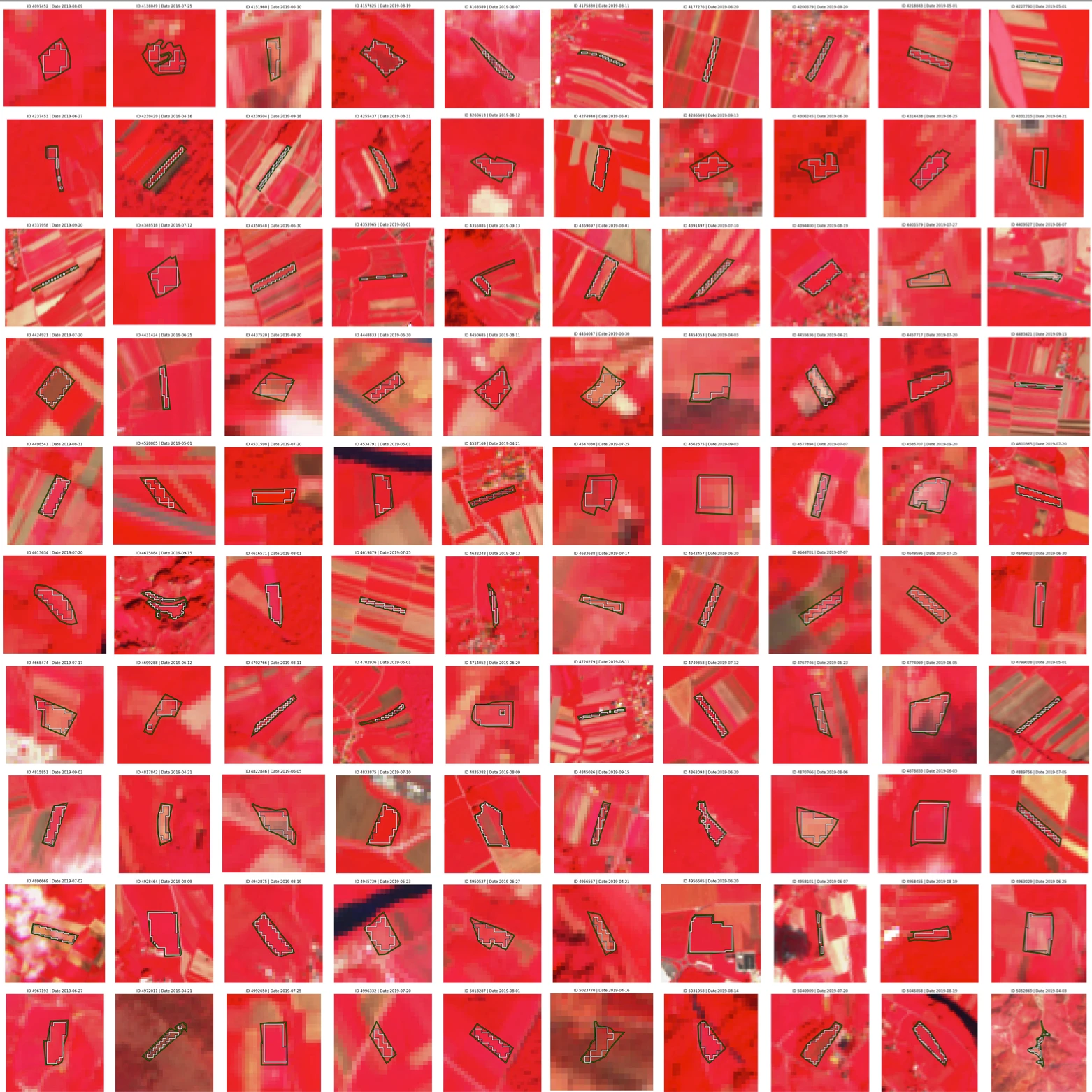
An error is displayed if it is not provided and the `signalTypes` prop contains elements with `signalTypeId` that **do not contain word `custom`**. | | `signalTypes`\* | `array` | | The array of objects with properties needed to get the data for correct signal types and if they are displayed or not, and how.
For more details see [signal types API in the signal marker visualization API component](#signal-types-api-in-the-signal-marker-visualization-api-component). | | `customSignalsData` | `object` | | For more details see [custom signals data API in the signal marker visualization API component](#custom-signals-data-api-in-the-signal-marker-visualization-api-component).
An error is displayed if it is not provided and the `signalTypes` prop contains elements with `signalTypeId` that **do contain word `custom`**. | | `markerServiceUrl` | `string` | | The (base) URL at which the endpoints for markers are (for example, `https://am-test.sinergise.com/marker/`). It can include the trailing slash, but it is not required.
It must be provided if `markers` prop is provided otherwise, an error is displayed. | | `markers` | `array` | | The array of objects with properties needed to get the correct markers and to know if they need to be displayed or not.
For more details see [markers API in the signal marker visualization API component](#markers-api-in-the-signal-marker-visualization-api-component). | | `onDateSelect` | callback `((onDateSelectEvent: OnDateSelectEvent) => void)` | | Callback that receives an object with a `value` of the selected date in `ISOString` format and `isExternal` with a `boolean` value (`true` value meaning that the event was triggered from outside by changing `selectedDate` prop). | | `selectedDate` | `string` | | The date in [ISO 8601](https://en.wikipedia.org/wiki/ISO_8601) format (for example, `YYYY-MM-DD`). | | `selectedDateColor` | `string` | `#ff0000` | The color of the vertical line that denotes the selected date.
Possible formats: `hex`, `rgb()`, `rgba()`, HTML color name/keyword. | | `language` | `string` | | The selected language at the time of rendering.
Options are: `sl` - Slovenian, `en` - English. | | `dateFormat` | `string` | | If not present and `language` is present will take the default selected language format. If both are not present defaults to `enUS` (for example, `d. m. yyyy`). For more details, see the [accepted format guide](https://date-fns.org/v2.29.2/docs/format). | *\* indicates mandatory props* ### Signal types API in the signal marker visualization API component The `signalTypes` prop contains an array of objects with properties needed to get the data for correct signal types and if they are displayed or not, and how they are displayed. It can contain elements for signal types from: * signal service (provided by `signalServiceUrl` parameter) * `customSignalsData` parameter The properties of an object in the array are listed in the table below. | Property | Type | Default | Description | | ------------------- | -------- | ------- | ---------------------------------------------------------------------------------------------------------------------------------------------------------------------------------- | | `signalTypeId`\* | `string` | | The fully qualified ID of a signal type. | | `shown`\* | `string` | | Shows (the value is `true`) or hides (the value is `false`) the signal on component load. | | `foiId`\* | `string` | | The fully qualified ID of a FOI (feature of interest; for example, `DEMO.FOI.7025947001`). | | `validSignalTypeId` | `string` | | The fully qualified ID.
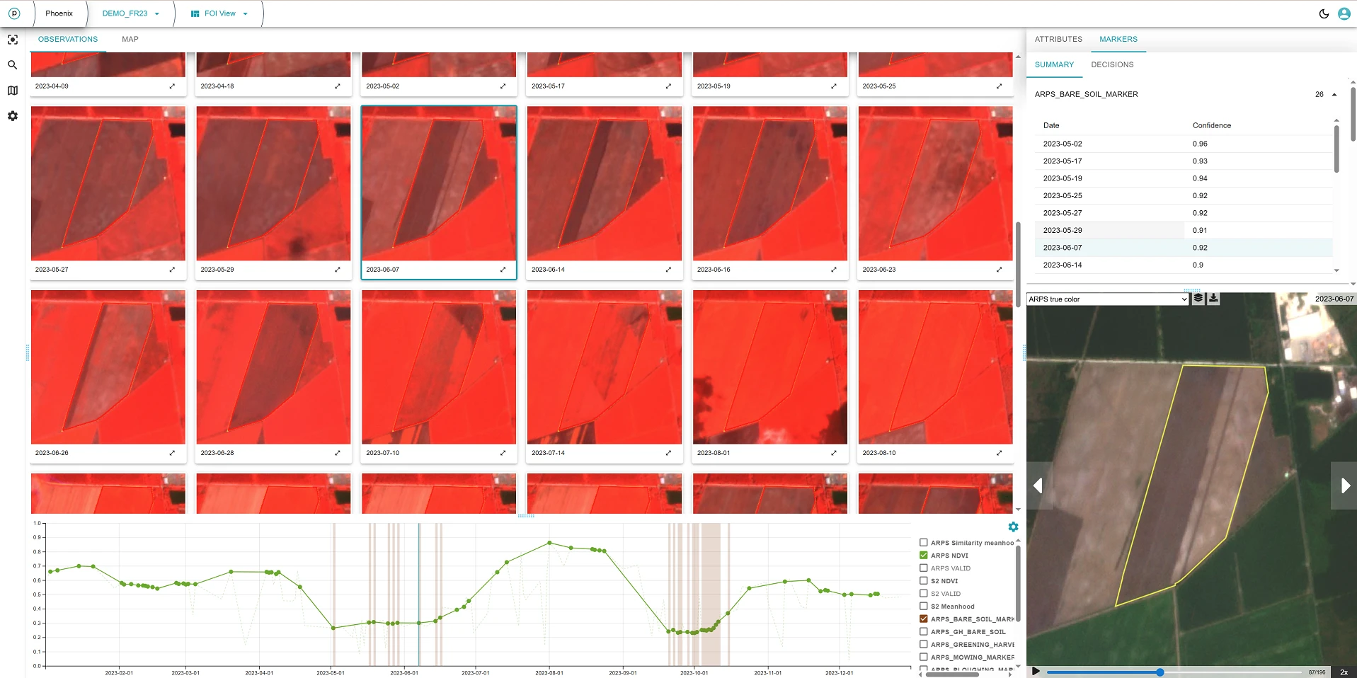
If provided it will be used instead of the default `validSignalTypeId` resolution from the signal code list. | | `label` | `string` | | The alternative text for the label in the legend and tooltips. | | `lineColor` | `string` | | The default color for the signal line.
Possible formats: `hex`, `rgb()`, `rgba()`, HTML color name/keyword. | | `bandColor` | `string` | | The color of the mean+-stDev band around the signal line.
Possible formats: `hex`, `rgb()`, `rgba()`, HTML color name/keyword.
If not provided, the `lineColor` is used. | | `bandOpacity` | `number` | `0.3` | The opacity of the mean+-stDev band around the signal line.
Possible value: number between `0` and `1`. | | `validColor` | `string` | | The color for the signal line between valid dates.
Possible formats: `hex`, `rgb()`, `rgba()`, HTML color name/keyword. If not provided, the `lineColor` is used. | *\* indicates mandatory properties* When multiple signals of the same `signalTypeGroup` are provided, the first one from the array will be used to remember the selection between different instances/sessions. ### Custom signals data API in the signal marker visualization API component The `customSignalsData` prop contains `signalTypes` and `signals` arrays. The `signalTypes` array must be formatted similarly to the response from the signal service (provided by `signalServiceUrl` parameter). Every element in the `signalTypes` array must contain the fields listed in the table below. Other fields in the element are ignored. | Field | Type | Description | | ------------------- | -------- | ------------------------------------------------------------------------------------------------------------------------------------------------------------------------------ | | `id`\* | `string` | Must contain word *"custom"*. | | `code`\* | `string` | Custom signal type code. | | `names` | `array` | It is needed if the `label` is not defined for the signal type in `signalTypes` prop. | | `signalClass`\* | `string` | For correct visualization - valid/invalid or mean +/- stDev. | | `validSignalTypeId` | `string` | It is needed for the visualization of valid/invalid signal data points.
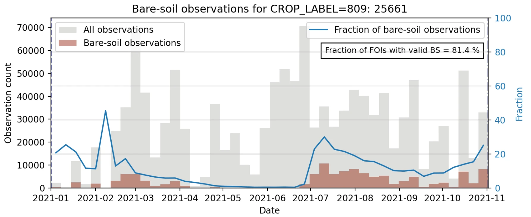
If `validSignalTypeId` in `signalTypes` prop is defined for the signal type, this one is ignored. | *\* indicates mandatory fields* The `signals` array must be formatted similarly to the response from the signal service (provided by `signalServiceUrl` parameter). Every element in the `signals` array must contain the fields listed in the table below. Other fields in the element are ignored. | Field | Type | Description | | ---------- | -------- | ------------------------------------------------------------------------------------------------- | | `id`\* | `string` | Must be the same as `id` in the element in the `signalTypes` array of `customSignalsData` prop. | | `code`\* | `string` | Must be the same as `code` in the element in the `signalTypes` array of `customSignalsData` prop. | | `values`\* | `array` | List of signal values. | *\* indicates mandatory fields* Every element in the `values` array must contain the fields listed in the table below. Other fields in the element are ignored. | Field | Type | Description | | --------- | -------- | ------------------------------------------------------------------------------------------------------------------------------------------- | | `time`\* | `string` | Date of the signal. | | `mean`\* | `number` | Mean value of the signal. | | `stDev`\* | `number` | It is needed for the signal types that are not used for the validation of data points. | | `value` | `number` | It is needed for the signal types that are not used for the validation of data points.
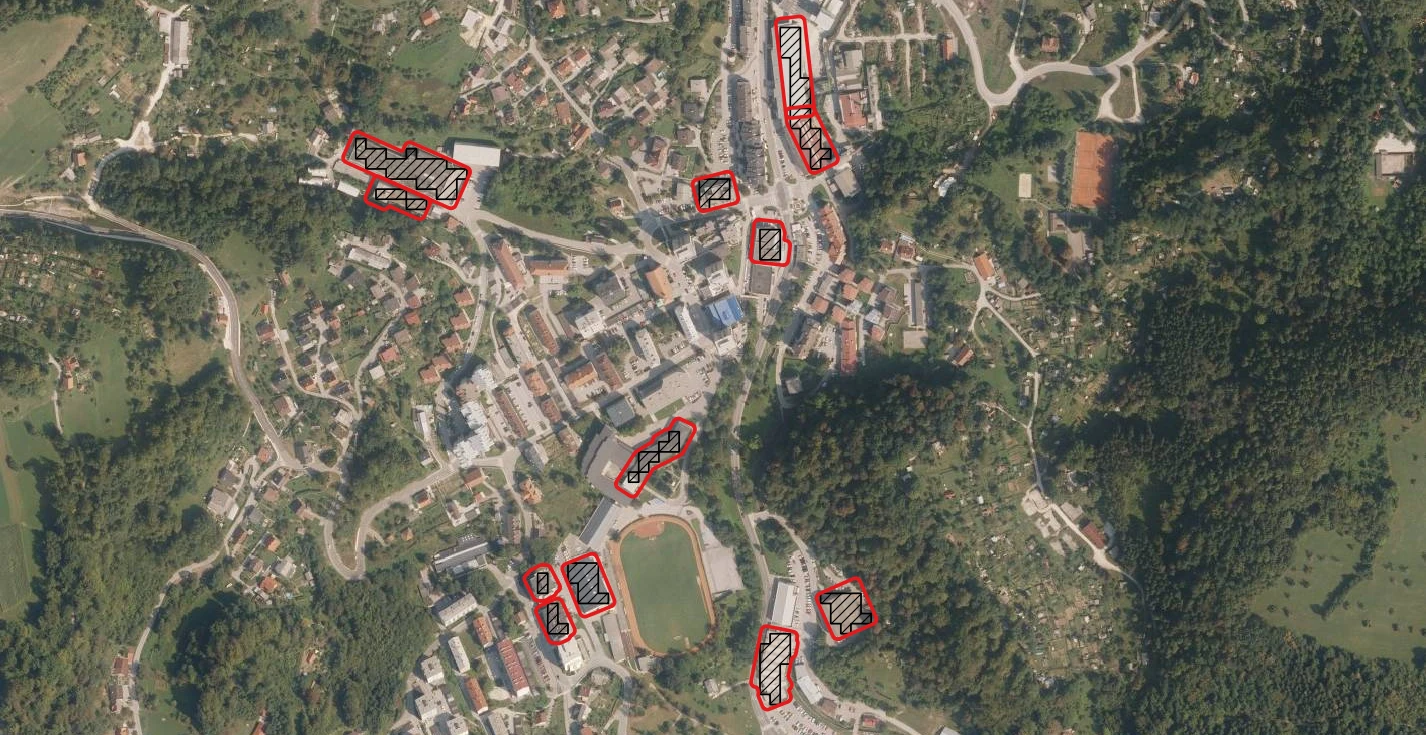
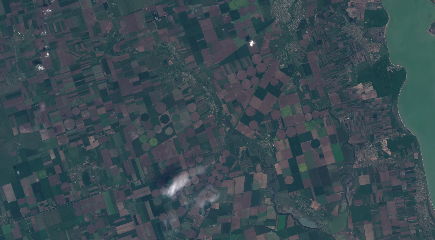
If it is not provided, the `mean` will be used. | *\* indicates mandatory fields* ### Markers API in the signal marker visualization API component The `markers` prop contains an array of objects with properties needed to get the correct markers and to know if they need to be displayed or not. The properties of an object in the array are listed in the table below. | Property | Type | Default | Description | | --------------- | -------- | ------- | -------------------------------------------------------------------------------------------------- | | `inferenceId`\* | `string` | | The fully qualified ID of an inference. Previously `markerTypeId` was used to get the marker data. | | `shown`\* | `string` | | Shows (the value is `true`) or hides (the value is `false`) the marker on component load. | | `foiId`\* | `string` | | The fully qualified ID of a FOI (feature of interest; for example, `DEMO.FOI.7025947001`). | | `label` | `string` | | The alternative text for the label in the legend and tooltips. | | `color` | `string` | | Possible formats: `hex`, `rgb()`, `rgba()`, HTML color name / keyword. | | `opacity` | `number` | `0.2` | Possible value: number between `0` and `1`. | *\* indicates mandatory properties* If there is no object defined for a marker type, the component will choose a random color. When multiple markers of the same markerTypeGroup are provided, the first one from the array will be used to remember the selection between different instances/sessions. **Example**: ``` [ { label: 'Inference 26 LABEL', // mandatory inferenceId: 'SI19.INFERENCE.26', // mandatory foiId: 'SI19.FOI.CROP_4106574', // mandatory shown: 'true', // mandatory color: '#396478', // optional opacity: 0.4, // optional }, ]; ``` --- Copy for LLM[View as Markdown](https://docs.planet.com/data/area-monitoring/visualizations/timelapse/) # Timelapse Timelapse *React* component displays the timelapse of the selected FOI image chips for the selected layer. Timelapse can either play through image chips automatically with a defined speed or the user can navigate it image chip by image chip. ![](/data/area-monitoring/visualizations/timelapse/timelapse_example.gif) ## User interactions The timelapse component has several elements with which the user can control it: * `(1)` drop-down list of layers to select a layer to be displayed in the timelapse component * `(2)` check-box list of FOI geometry types (original, pixelated) to be displayed in timelapse component * `(3)` button to generate and download timelapse GIF animation through all image chips * `(4)` date of the currently displayed image chip in the timelapse component * `(5)`/`(6)` button to manually navigate the timelapse component to the previous/next image chip * `(7)` button to play/pause timelapse animation through all image chips * `(8)` slider to manually navigate timelapse component through image chips * `(9)` sequence number of current image chip and number of all image chips * `(10)` button to control the speed of timelapse animation ![](/data/area-monitoring/visualizations/timelapse/timelapse_elements.webp) ## Timelapse API ### Usage ``` console.log('Date was selected:', date)} geometries={[ { geometry: geoJSONGeometry1, style: { strokeColor: 'white', lineWidth: 1, }, id: 'field', label: 'Field', }, { geometry: geoJSONGeometry2, style: { strokeColor: 'red', lineWidth: 1, }, id: 'pixelated', label: 'Pixelated field', }, ]} autoplay={true} paddingXPercent={10} paddingYPercent={10} width={450} height={350} enableGifExport={true} language="sl" dateFormat="DD/MM/YYYY" upsampling="BICUBIC" downsampling="BICUBIC" cacheDuration={300} /> ``` ### Component name The component name `Timelapse` should be used when providing the [*props*](#props). ### Props The *props* of the Timelapse *React* component are described in the table below. | Name | Type | Default | Description | | ----------------------- | --------------------------------------------------------------------------------------------------- | ------- | -------------------------------------------------------------------------------------------------------------------------------------------------------------------------------------------------------------------------------------------------------------------------------------- | | `baseUrl`\* | `string` | | Contains an OGC WMS compatible base URL address (for example, `https://services.sentinel-hub.com/ogc/wms/`). The address needs to support `GetCapabilities` call. | | `layers`\* | `array` | | Defines layers that can be displayed. For more details see [layers API in the timelapse API component](#layers-api-in-the-timelapse-api-component). | | `geometries`\* | `array` | | Defines geometries to be displayed. For more details see [the geometries API in the timelapse API component](#geometries-api-in-the-timelapse-api-component). | | `shAuthToken`\* | `string` or callback `(() => string)` | | Sentinel Hub authentication token. Either as a string or a function that returns a string. If using [sentinelhub-js](https://github.com/sentinel-hub/sentinelhub-js/), it can be obtained using `requestAuthToken` function. | | `amServicesAuthToken`\* | `string` or callback `(() => string)` | | AM services authentication token. Either as a string or a function that returns a string. | | `signalServiceUrl`\* | `string` | | The (base) AM signal service URL at which the endpoints for signals are (for example, `https://am-test.sinergise.com/signal/`). | | `scope`\* | `string` | | Reference data differentiator (for example, `SI22`). For more details see the [scope](https://docs.planet.com/data/area-monitoring/common.md#scope). | | `foiId`\* | `string` | | Fully qualified ID of a FOI (feature of interest; for example, `DEMO.FOI.7025947001`). | | `defaultTimespan`\* | `object` | | The default date range. Only used until a change is saved to `localStorage`. Fields `from` and `to` are strings that represent a date in [ISO 8601](https://en.wikipedia.org/wiki/ISO_8601) format (for example, `{ from: '2020-01-01', to: '2020-01-31' }`). | | `width` | `number` or `string` | `100%` | Width (for example, `300`) of the component (and thus images) in pixels. | | `height` | `number` or `string` | `100%` | Height (for example, `300`) of the component (and thus images) in pixels. | | `paddingXPercent` | `number` or `string` | `10` | Percent of padding in the horizontal direction (for example, `10`). | | `paddingYPercent` | `number` or `string` | `10` | Percent of padding in the vertical direction (for example, `10`). | | `dateFormat` | `string` | | Date format (for example, `d. m. yyyy`). If not present and `language` is present, it will take the default selected language format. If both are not present defaults to `enUS`. See the accepted format guide [here](https://date-fns.org/v2.29.2/docs/format). | | `upsampling` | `string` | | Upsampling interpolator for image chip. Available options: `BILINEAR`, `BICUBIC`, `NEAREST` | | `downsampling` | `string` | | Downsampling interpolator for image chip. Available options: `BILINEAR`, `BICUBIC`, `NEAREST` | | `selectedDate` | `string` - compatible with [ISO 8601](https://en.wikipedia.org/wiki/ISO_8601) format (`YYYY-MM-DD`) | | Contains the UTC date (for example, `2021-03-31`) that is used for the background image. If no image is available for this date then it will show the closest available image. | | `onDateSelect` | callback `((value: string \| null) => void)` | | Callback that receives a string or null value. | | `useValidSignal` | `boolean` (`true`/`false`) | | Indicator if all or only valid image chips should be displayed. For more details see [useValidSignal](#usevalidsignal). | | `autoplay` | `boolean` (`true`/`false`) | | Initial timelapse animation playing state setting when the component mounts for the first time. On subsequent loads, this setting is loaded from the browser's local storage. | | `lazyLoading` | `boolean` (`true`/`false`) | | If not present or if it is `false`, the timelapse will try to download all images. If it is `true`, timelapse will download only the first image, other images will be downloaded when the left/right arrow is pressed or when the animation is started by clicking the *play* button. | | `enableGifExport` | `boolean` (`true`/`false`) | | If `true`, it shows the button for exporting the timelapse animation as GIF. If `false` or not set, the button is not shown. | | `gifFilename` | `string` | | If provided, the exported GIF file will have that name (for example, `my_animation.gif`). If not provided, the exported GIF file will be named `timelapse.gif`. | | `language` | `string` | `en` | The selected language. Available options: `sl` - Slovenian, `en` - English, `de` - German | | `cacheDuration` | `number` or `string` | `300` | Cache duration in seconds (for example, `500`). | *\* indicates mandatory props* #### `useValidSignal` If not present or if it is `false`, the Timelapse will show images for all available dates from Sentinel Hub for the selected layer and area (around geometries) within the selected time range. If it is `true`, the Timelapse will filter out images for the dates that are marked as invalid in the response to AM signal service. The remaining dates will be the images for the dates that are not present in the response from AM signal service or are present and marked as valid. ### Layers API in the timelapse API component The `layers` prop contains an array of objects. The sort order of this array is not important, objects are sorted by `layerId` (alphabetically). Every object in the array contains properties described in the table below. | Property | Type | Description | | ------------------- | -------- | -------------------------------------------------------------------------------------------------------------------------------------------------------------------------------------------------------------------------------------------------------------------------------------------------------------------------------------------------------------------------------------------------------------------------------------------- | | `layerId`\* | `string` | Layer ID. Must be available at the `baseUrl` specified (unknown `layerId` is silently ignored - not available for selection in the component drop-down list). | | `validSignalTypeId` | `string` | Valid signal type ID in fully qualified identifier form. Must be available at the `signalServiceUrl` specified (unknown `validSignalTypeId` is silently ignored - invalid dates will not be filtered out). | | `geometryIds` | `array` | Contain the same `id`s as in `geometries` prop, the order is not important:
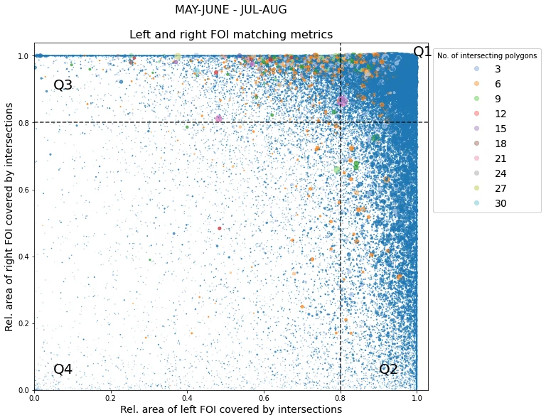
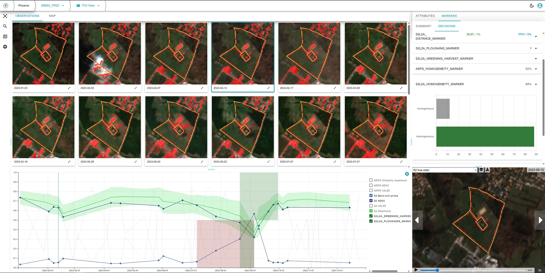
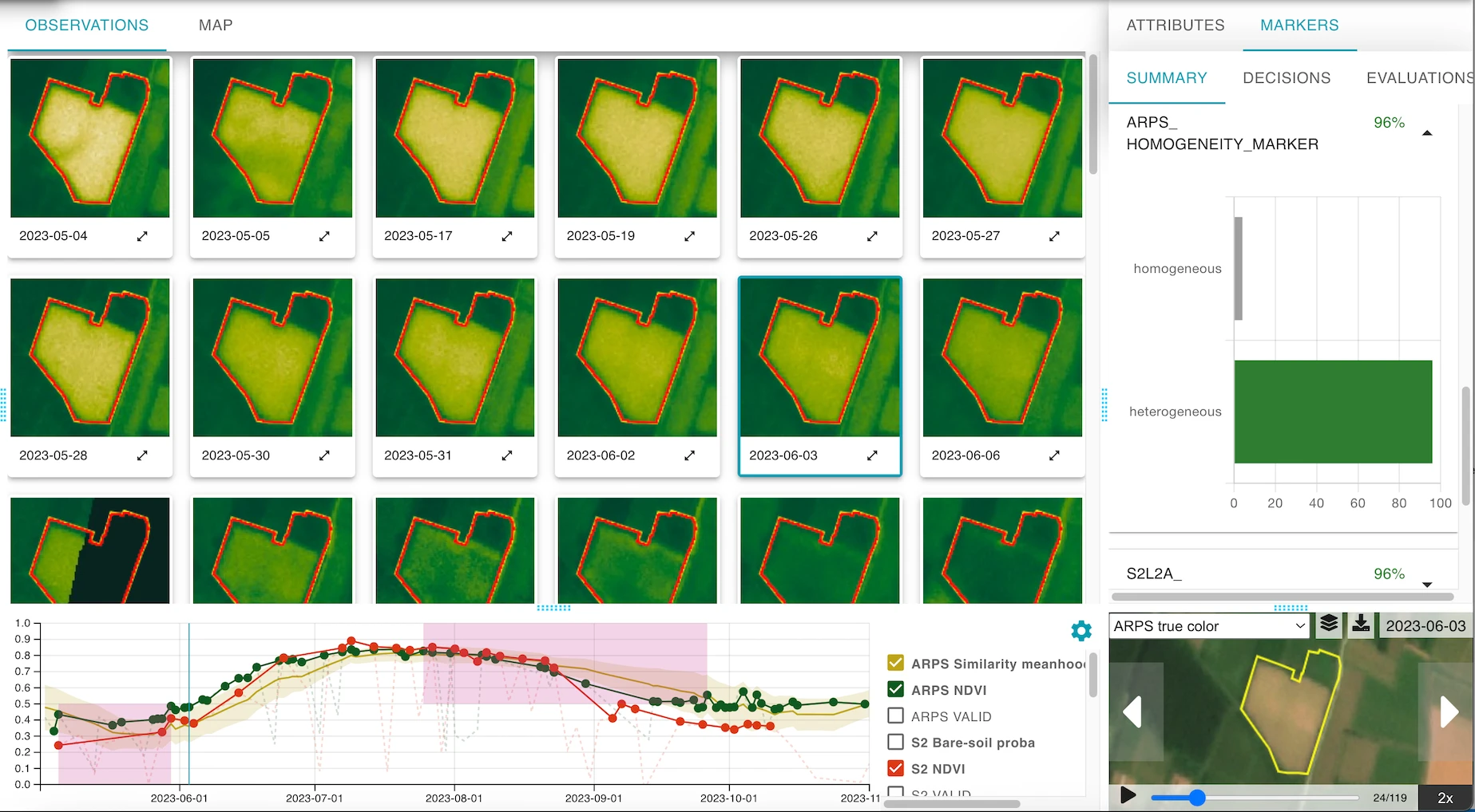
- if not present, all geometries in `geometries` will be rendered
- if `undefined`, `null` or `[]` (empty array), no geometries will be rendered
- if containing correct geometry IDs, the geometries with those IDs will be rendered
- if containing one or more IDs that no geometry in `geometries` parameter has, an error will be shown | *\* indicates mandatory properties* note Note that while there is no requirement that layer and valid signal type from the same object use the same collection, the dates for a valid signal type are only valid for a specific collection. In practice, the layer and valid signal type from the same object should be using the same collection. **Example** `layers`: ``` layers={[ { layerId: 'MY_LAYER_1', validSignalTypeId: 'VALID_SIGNAL_1', geometryIds: [ 'field', 'pixelated' ], }, { layerId: 'MY_LAYER_2', validSignalTypeId: 'VALID_SIGNAL_2', geometryIds: [ 'field' ], }, ]} ``` ### Geometries API in the timelapse API component The `geometries` prop contains an array of objects. Every object in the array contains properties described in the table below. | Property | Type | Description | | ------------ | -------- | ----------------------------------------------------------------------------------------------------------------------------------------------------------------------------------------------------------------------------------- | | `geometry`\* | `object` | Geometry to be displayed in the timelapse component. See [Geometry](https://docs.planet.com/data/area-monitoring/common.md#geometry) for more details. | | `style`\* | `object` | Style in which geometry is to be displayed in the timelapse component. See [Style](https://docs.planet.com/data/area-monitoring/common.md#style) for more details. | | `id`\* | `string` | Geometry ID. Allows the user to show/hide geometries. Note that the shown IDs are saved globally, so if another component is mounted with a different set of geometry `id`s, they will be hidden (until selected through settings). | | `label`\* | `string` | Geometry label. | *\* indicates mandatory properties* **Example** `geometries`: ``` geometries={[ { geometry: { type: 'MultiPolygon', coordinates: [ [ [ [11.02, 45.01], [11.02, 45.02], [11.03, 45.02], [11.03, 45.01], [11.02, 45.01], ], ], ], }, style: { strokeColor: 'white', lineWidth: 2, }, id: "field", label: "Field", }, ... ]} ``` --- Copy for LLM[View as Markdown](https://docs.planet.com/data/imagery/) # Planet Imagery [![](/data/imagery/arps/arps-2022-brazil-publish.gif)](https://docs.planet.com/data/imagery/arps.md) ### [Analysis-Ready PlanetScope](https://docs.planet.com/data/imagery/arps.md) [Information about Analysis-Ready PlanetScope](https://docs.planet.com/data/imagery/arps.md) [![](/data/imagery/mosaics/thumbnail.webp)](https://docs.planet.com/data/imagery/mosaics.md) ### [Mosaics](https://docs.planet.com/data/imagery/mosaics.md) [Information about Mosaics](https://docs.planet.com/data/imagery/mosaics.md) [![](/data/imagery/pelican/thumbnail.webp)](https://docs.planet.com/data/imagery/pelican.md) ### [Pelican](https://docs.planet.com/data/imagery/pelican.md) [Information about the Pelican Constellation](https://docs.planet.com/data/imagery/pelican.md) [![](/data/imagery/planetscope/thumbnail.webp)](https://docs.planet.com/data/imagery/planetscope.md) ### [PlanetScope](https://docs.planet.com/data/imagery/planetscope.md) [Information about the PlanetScope Constellation](https://docs.planet.com/data/imagery/planetscope.md) [![](/data/imagery/rapideye/re_thumbnail.webp)](https://docs.planet.com/data/imagery/rapideye.md) ### [RapidEye](https://docs.planet.com/data/imagery/rapideye.md) [Information about the RapidEye Constellation](https://docs.planet.com/data/imagery/rapideye.md) [![](/data/imagery/skysat/thumbnail.webp)](https://docs.planet.com/data/imagery/skysat.md) ### [SkySat](https://docs.planet.com/data/imagery/skysat.md) [Information about the SkySat Constellation](https://docs.planet.com/data/imagery/skysat.md) [![](/data/imagery/superres/central-park-manhattan-new-york-super-res.webp)](https://docs.planet.com/data/imagery/superres.md) ### [SuperRes](https://docs.planet.com/data/imagery/superres.md) [Information about SuperRes imagery.](https://docs.planet.com/data/imagery/superres.md) [![](/data/imagery/tanager/tanager-plume.webp)](https://docs.planet.com/data/imagery/tanager.md) ### [Tanager](https://docs.planet.com/data/imagery/tanager.md) [Information about the Tanager Constellation](https://docs.planet.com/data/imagery/tanager.md) [![](/data/imagery/udm/clouds_shropshire_england_20231103_101837_21_2455_toar_with_cloud_map_6m_CLOUDS_flat_rotated_2880px_geo.webp)](https://docs.planet.com/data/imagery/udm.md) ### [Usable Data Mask](https://docs.planet.com/data/imagery/udm.md) [Information about UDM data](https://docs.planet.com/data/imagery/udm.md) --- Copy for LLM[View as Markdown](https://docs.planet.com/data/imagery/arps/) # Analysis-Ready PlanetScope ![Header Thumbnail](/data/imagery/arps/arps-2022-brazil-publish.gif) ## About Analysis-Ready PlanetScope This product includes derived imagery from [PlanetScope](https://docs.planet.com/data/imagery/planetscope.md) sensors. Analysis-Ready PlanetScope combines data from the three available PlanetScope sensors (Dove Classic, Dove-R, and SuperDove) while enhancing temporal and spatial consistency with trusted, third-party data sources (Landsat, Sentinel-2, MODIS, VIIRS). This is accomplished with a proprietary algorithm that creates pre-processed, harmonized, and spatially consistent near-daily stacks of images that enable time-series analysis and machine learning applications. It delivers four surface reflectance bands: blue, green, red, and near-infrared. The earliest Analysis-Ready PlanetScope imagery is available on January 01, 2017. The product is produced on demand when a subscription is initiated. ## Product Overview Planet offers Analysis-Ready PlanetScope (ARPS) imagery as a 3 m orthorectified (corrected for terrain distortions) surface reflectance product (ARP-SR). The data is stored in 16-bit integer format (with a multiplication factor of 10,000) as cloud-optimized geotiffs compressed using LZW compression. During processing and harmonization, 4-band PS TOA Reflectance (PS-TOAR) (converted from the radiances) are transformed into surface reflectances, ensuring radiometric consistency with FORCE-processed Sentinel-2 and Landsat. As a result, the spectral bands and spectral response functions of ARPS data will be equivalent to the blue (B2), green (B3), red (B4), and narrow NIR (B8a) bands of Sentinel-2 (ESA 2024). The surface reflectance data represent Normalized BRDF Adjusted Reflectances (NBAR) as the Landsat 8/9 and Sentinel-2 data used for cross-calibration have been normalized to the nadir view. Enhanced geometric performance includes temporal positional accuracy of <4m RMSE PCTL90. The surface reflectance product is accompanied by a Quality Assurance product (ARP-QA) in GeoTIFF format. The QA product is a 2-layer thematic raster using the same spatial grid as the corresponding Analysis-Ready PlanetScope spectral data. Layer 1, Cloud and shadow mask, contains information denoting usable data using seven classifications that allow users to remove pixels that are not useful after they download the image. Layer 2, Pixel provenance has integers that can be mapped to PlanetScope scene IDs using the information in the QA raster's metadata header. Analysis-Ready PlanetScope products are projected in the UTM zone intersected by their extent using the WGS-84 horizontal datum. ### Available IDs Analysis-Ready PlanetScope can be requested using the Subscriptions API. The following products can be requested with the associated ID. Please note that at this time, Analysis-Ready PlanetScope does not support MultiPolygon geometry. Subscriptions can only be created using Polygon geometry. For more details on how to subscribe to Analysis-Ready PlanetScope, please visit the [Subscriptions API](https://docs.planet.com/develop/apis/subscriptions/sources.md#planetary-variable-and-analysis-ready-source-types) documentation. Loading resource data... Loading... ## Available Bands and Data This section explains the bands and data which can be set in the evalscript input object. Any string listed in the **Name** column can be an element of the `input.bands` array in your evalscript. Analysis-Ready PlanetScope data is delivered with two assets: surface reflectance (SR) and quality assurance (QA). | Name | Description | Resolution | | ----------- | ------------------------------------------------ | ---------- | | blue | Blue band | 3 m | | green | Green band | 3 m | | red | Red band | 3 m | | nir | Near-infrared band | 3 m | | cloud\_mask | Cloud and shadow mask | 3 m | | scene\_mask | Pixel provenance (maps to PlanetScope scene IDs) | 3 m | ## Units The data values for each band in your evalscript are provided in the units specified below. Surface reflectance bands are stored as 16-bit integers with a multiplication factor of 10,000. To convert digital numbers (DN) to reflectance values, use the following formula: ``` reflectance = DN / 10000 ``` For example, a DN value of 2500 corresponds to a reflectance of 0.25. | Band | Physical Quantity (units) | Data Type | No Data Value | Typical Range | | ------------------------------------- | ----------------------------- | --------- | ------------- | ----------------------------------------------------------------------------------------------------------------------------------------------------------------------------------------------- | | Optical bands (blue, green, red, nir) | Scaled reflectance (unitless) | int16 | 0 | 0 - 4000. Highly reflective pixels can have values up to 10000. | | cloud\_mask | Cloud mask (unitless) | int16 | -999 | 1 - clear
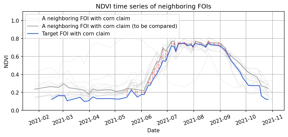
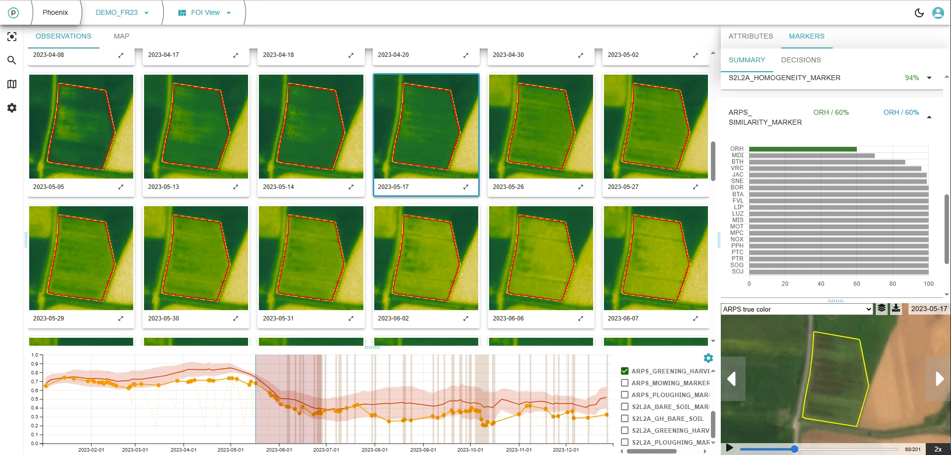
2 - bright cloud
3 - cloud shadows
4 - haze
5 - adjacent clouds or cloud shadows
6 - additional haze or cloud elements
7 - contamination including snow | | scene\_mask | Pixel provenance (unitless) | int16 | -999 | 0 - 1000 | ## Examples For Processing API request examples, including true color, false color, NDVI calculations, and GeoTIFF exports, see [Processing API Examples - ARPS](https://docs.planet.com/develop/apis/processing/examples.md#analysis-ready-planetscope-examples). --- Copy for LLM[View as Markdown](https://docs.planet.com/data/imagery/arps/sandbox/) # Analysis-Ready PlanetScope Sandbox Data This Planet Sandbox Data collection for Analysis-Ready PlanetScope provides sample data over specific areas and times of interest. The data is available to paid and trial accounts that include processing units and is available under the CC-BY-NC license. Learn more about [Planet Sandbox Data](https://docs.planet.com/data/planet-sandbox-data.md). ## Data Collections Metadata | Source ID | Collection Name | Collection ID | Time Range | | ------------------ | ------------------------------------------------ | ----------------------------------------- | ----------------------- | | PS\_ARD\_SR\_DAILY | Planet Sandbox Data - Analysis Ready PlanetScope | BYOC-3f605f75-86c4-411a-b4ae-01c896f0e54e | 2021-01-01 - 2023-12-31 | ## Planet Sandbox Data Areas This collection includes 22 sandbox regions. Download the GeoJSON file below the map for exact polygon boundaries. View all 22 regions | Location | Area (km²) | Time Range | Center (lat, lon) | | ------------------------------------------------- | ---------- | ----------------------- | ----------------- | | Arizona, United States | 576 | 2022-01-01 – 2023-12-31 | 32.86, -111.86 | | Alberta, Canada | 576 | 2022-01-01 – 2023-12-31 | 50.15, -111.78 | | Iowa, United States | 2306 | 2021-01-02 – 2023-12-30 | 41.19, -93.81 | | Cusco, Province of Chumbivilcas, Peru | 575 | 2021-01-04 – 2023-12-31 | -14.56, -71.75 | | Pará, North Region, Brazil | 576 | 2021-01-01 – 2023-12-29 | -6.77, -52.38 | | Goiás, Central-West Region, Brazil | 576 | 2022-01-02 – 2023-12-30 | -16.52, -48.83 | | Autonomous Community of the Basque Country, Spain | 576 | 2022-01-01 – 2023-12-31 | 42.81, -2.51 | | Nouvelle-Aquitaine, Metropolitan France, France | 2304 | 2021-01-01 – 2023-12-27 | 44.84, -0.52 | | Flevoland, Netherlands | 576 | 2022-01-03 – 2023-12-01 | 52.50, 5.71 | | Groningen, Netherlands | 1000 | 2022-01-03 – 2023-12-30 | 53.14, 6.24 | | Emilia-Romagna, Italy | 576 | 2022-01-01 – 2023-12-25 | 44.97, 9.81 | | Brandenburg, Germany | 576 | 2021-01-14 – 2023-12-30 | 52.30, 13.47 | | Epirus and Western Macedonia, Greece | 576 | 2022-01-01 – 2023-12-30 | 40.65, 21.76 | | Attica, Greece | 576 | 2022-01-01 – 2023-12-31 | 38.02, 23.92 | | Al Qalyubiya, Egypt | 576 | 2021-01-01 – 2023-12-31 | 30.25, 31.17 | | Kitui County, Kenya | 576 | 2022-01-01 – 2023-12-31 | -1.34, 37.85 | | Al Jawf Region, Saudi Arabia | 576 | 2022-01-01 – 2023-12-27 | 30.05, 38.42 | | Haryana, India | 576 | 2022-01-01 – 2023-12-26 | 27.86, 77.36 | | Hưng Yên Province, Vietnam | 576 | 2022-01-02 – 2023-12-31 | 20.51, 106.30 | | Guizhou, Tongren, China | 576 | 2022-01-11 – 2023-12-30 | 28.09, 109.21 | | Western Australia, Australia | 576 | 2021-01-01 – 2023-12-31 | -31.92, 116.15 | | New South Wales, Australia | 576 | 2022-01-02 – 2023-12-31 | -34.52, 146.13 | [Download GeoJSON](https://docs.planet.com/data/imagery/arps/polygons.geojson) ## Highlights [![Des Moines, United States](/data/imagery/arps/ARPS_Des_Moines.webp)](https://insights.planet.com/analyze/browser/?zoom=12\&lat=41.3\&lng=-93.9558\&themeId=PLANET_SANDBOX\&visualizationUrl=https%3A%2F%2Fservices.sentinel-hub.com%2Fogc%2Fwms%2F23b2442b-a5bb-42b5-87cd-916e28c34a5e\&datasetId=3f605f75-86c4-411a-b4ae-01c896f0e54e\&fromTime=2023-04-19T00%3A00%3A00.000Z\&toTime=2023-04-19T23%3A59%3A59.999Z\&layerId=0_TRUE-COLOR-CLOUDMASKED\&demSource3D=%22MAPZEN%22) Des Moines, United States 2021-01-01 - 2023-12-31
576km² [Visualize in the Browser →](https://insights.planet.com/analyze/browser/?zoom=12\&lat=41.3\&lng=-93.9558\&themeId=PLANET_SANDBOX\&visualizationUrl=https%3A%2F%2Fservices.sentinel-hub.com%2Fogc%2Fwms%2F23b2442b-a5bb-42b5-87cd-916e28c34a5e\&datasetId=3f605f75-86c4-411a-b4ae-01c896f0e54e\&fromTime=2023-04-19T00%3A00%3A00.000Z\&toTime=2023-04-19T23%3A59%3A59.999Z\&layerId=0_TRUE-COLOR-CLOUDMASKED\&demSource3D=%22MAPZEN%22) [![Bordeaux, France](/data/imagery/arps/ARPS_Bordeaux.webp)](https://insights.planet.com/analyze/browser/?zoom=12\&lat=44.73491\&lng=-0.67566\&themeId=PLANET_SANDBOX\&visualizationUrl=https%3A%2F%2Fservices.sentinel-hub.com%2Fogc%2Fwms%2F23b2442b-a5bb-42b5-87cd-916e28c34a5e\&datasetId=3f605f75-86c4-411a-b4ae-01c896f0e54e\&fromTime=2023-04-18T00%3A00%3A00.000Z\&toTime=2023-04-18T23%3A59%3A59.999Z\&layerId=0_TRUE-COLOR-CLOUDMASKED\&demSource3D=%22MAPZEN%22) Bordeaux, France 22021-01-01 - 2023-12-31
576km² [Visualize in the Browser →](https://insights.planet.com/analyze/browser/?zoom=12\&lat=44.73491\&lng=-0.67566\&themeId=PLANET_SANDBOX\&visualizationUrl=https%3A%2F%2Fservices.sentinel-hub.com%2Fogc%2Fwms%2F23b2442b-a5bb-42b5-87cd-916e28c34a5e\&datasetId=3f605f75-86c4-411a-b4ae-01c896f0e54e\&fromTime=2023-04-18T00%3A00%3A00.000Z\&toTime=2023-04-18T23%3A59%3A59.999Z\&layerId=0_TRUE-COLOR-CLOUDMASKED\&demSource3D=%22MAPZEN%22) [![Perth, Australia](/data/imagery/arps/ARPS_Perth.webp)](https://insights.planet.com/analyze/browser/?zoom=12\&lat=-31.9137\&lng=116.1481\&themeId=PLANET_SANDBOX\&visualizationUrl=https%3A%2F%2Fservices.sentinel-hub.com%2Fogc%2Fwms%2F23b2442b-a5bb-42b5-87cd-916e28c34a5e\&datasetId=3f605f75-86c4-411a-b4ae-01c896f0e54e\&fromTime=2023-04-29T00%3A00%3A00.000Z\&toTime=2023-04-29T23%3A59%3A59.999Z\&layerId=0_TRUE-COLOR-CLOUDMASKED\&demSource3D=%22MAPZEN%22) Perth, Australia 2021-01-01 - 2023-12-31
576km² [Visualize in the Browser →](https://insights.planet.com/analyze/browser/?zoom=12\&lat=-31.9137\&lng=116.1481\&themeId=PLANET_SANDBOX\&visualizationUrl=https%3A%2F%2Fservices.sentinel-hub.com%2Fogc%2Fwms%2F23b2442b-a5bb-42b5-87cd-916e28c34a5e\&datasetId=3f605f75-86c4-411a-b4ae-01c896f0e54e\&fromTime=2023-04-29T00%3A00%3A00.000Z\&toTime=2023-04-29T23%3A59%3A59.999Z\&layerId=0_TRUE-COLOR-CLOUDMASKED\&demSource3D=%22MAPZEN%22) --- Copy for LLM[View as Markdown](https://docs.planet.com/data/imagery/arps/techspec/v1-0-0/) # Technical Specification v1.0 note This is the **v1.0 technical specification**, applicable to customers who received ARPS data produced with pipeline versions 1.0.0 and 1.0.1. The current specification is [Technical Specification](https://docs.planet.com/data/imagery/arps/techspec/v1-1-0.md) (v1.1.0). **SURFACE REFLECTANCE** v1.0.0, October 2024 ## 1. Analysis-Ready Planetscope Overview The PlanetScope (PS) constellation of 180+ CubeSats in low earth orbits represents a novel observational resource, which when combined with advances in conventional spaceborne sensing has resulted in a proliferation of satellite sensor data with unprecedented spatial, temporal, and spectral resolution. This constitutes a revolution in the ability to derive time-critical, location-specific insights about dynamic land surface processes. However, the potential for these systems to support decision making is often limited by sensor interoperability issues ([Figure 1](#kz1mqwbgovxc)), cross-calibration challenges, and atmospheric contamination. These obstacles can stand in the way of realizing the full potential of these rich datasets. ![Figure 1: Sources of interoperability issues.](/data/imagery/arps/figure-1.webp) *Figure 1: Sources of interoperability issues. Left: The reflectance field of the same observation target can appear very different at the point of the satellite sensor due to differences in satellite viewing and sun illumination angles augmented by shadow effects and non-lambertian surface characteristics (For example, as described by the Bidirectional Reflectance Distribution Function; BRDF). Right: Differences in spectral bands and spectral response functions can result in poor sensor interoperability. This is particularly pronounced when comparing Dove-C (For example, first generation PlanetScope) with public sensor sources (For example, L8).* Planet implemented and improved a rigorous methodology to enhance, harmonize, inter-calibrate, and fuse cross-sensor data streams. The CubeSat-Enabled Spatio-Temporal Enhancement Method (CESTEM) ([Houborg and McCabe 2018a](#8gfufoj8ok4f), [2018b](#xr6pcawhkolt)) leverages rigorously calibrated publicly accessible multispectral satellites (For example, Sentinel, Landsat, MODIS, VIIRS) to work in concert with the higher spatial and temporal resolution data provided by the Planet Dove CubeSats. The result is a next-generation, analysis-ready, harmonized Level-3 data product, which delivers a clean (For example, clouds and cloud shadows clearly labeled), temporally consistent, and radiometrically accurate 4-band surface reflectance (SR) data product. Analysis-Ready PlanetScope (ARPS) combines distributed observations from the hundreds of individual sensors that make up the PlanetScope constellation (using three generations of hardware). These observations are radiometrically and geometrically harmonized with each other while ensuring radiometric consistency with a suite of widely used reference satellite platforms. The result is a highly temporally consistent stack of PlanetScope data. This next-generation Analysis Ready Data (ARD) product is suitable for analytic and data science purposes. Analysis-Ready PlanetScope involves significant processing and novel methodology in the attempt to create a unique surface reflectance product enhanced in resolution, quality, and interoperability ([Figure 2](#xu3wgds3r48h)), as the pathway to useability and meaningful remote sensing driven insights. ![Figure 2: NDVI time series over a crop field near Lincoln (NE).](/data/imagery/arps/figure-2.webp) *Figure 2: Normalized Difference Vegetation Index (NDVI) time series over a crop field near Lincoln (NE) over the course of two years (July 2021 - July 2023). The ARPS processing translates original PlanetScope Top Of Atmosphere (TOA) reflectance inputs into Surface Reflectances (SR) consistent with Landsat 8/9 and Sentinel-2 clear-sky observations. Note the increased harmonization amongst ARPS observations and FORCE as compared to PlanetScope SR.* The unique features of Analysis-Ready PlanetScope can be summarized as: * **Advanced radiometric harmonization which leverages rigorously calibrated third-party sensors (MODIS/VIIRS, Landsat 8/9, and Sentinel-2) for full fleet interoperability** * **Rigorous, temporally driven, cloud and cloud shadow detection** * **Cleaned (For example, with cloud mask included) Surface Reflectance values delivered with a 48 hour latency** * **CubeSats with near-nadir field of view result in minimal BRDF variation effects** * **Designed to provide high radiometric accuracy and spatio-temporal consistency** * **Geometric harmonization with sub-pixel co-registration/alignment of disparate image sources** * **Includes pixel traceability information to identify source imagery for every data point** ## 2. Analysis-Ready Planetscope Inputs [Table 1](#eayvkhwt1aol) lists the data sources currently used in Analysis-Ready PlanetScope (ARPS) production. The Planet collection of 180+ CubeSats operates in sun synchronous orbits (altitude \~475 km) with a midmorning equatorial overpass time (9:30–11:30 a.m., local solar time) providing global near-nadir (\~4° field of view) imaging on a near-daily basis ([Roy et al., 2021](#nfg7qgvzajyq)). Three generations of "Doves" (collectively referred to as "PlanetScope" in this document) are used as input to ARPS products; the Dove-Classic constellation (2016-2022) is characterized by broad and partly overlapping spectral bands in the visible and near-infrared (NIR) spectrum ([Figure 1](#kz1mqwbgovxc)), whereas the Dove-R (2019-2022) and SuperDove (2020-) constellations are improved to be directly interoperable with the visible and narrow NIR bands of Sentinel-2. The nominal ortho scene size (at 475 km altitude) is also larger for Dove-R (\~25 km x 23 km) and SuperDove (\~32.5 km x 19.6 km) relative to Dove-Classic (\~25 km x 11.5 km). PlanetScope Top Of Atmosphere (TOA) Radiance inputs contribute the bulk of the observations used to make ARPS, and they are derived from 4-band Orthorectified Scene Products that have a resampled pixel size of 3 m (the ground sampling distance depends on the altitude and generation of each satellite and ranges from 3.7 to 4.2 m). While the SuperDove is an 8-band sensor (For example, it adds bands in the visible and red-edge domain compared to previous generations of Doves), currently only the blue, green, red, and NIR bands are used in ARPS production. []() **Table 1: List of inputs currently used in Analysis-Ready PlanetScope production.** | Product | Description | | ------------------- | ------------------------------------------------------------------------------------------------------------------------------------------------------------------------------------------------------------------------------------------------------------------------------------------------------------------------------------------------------------------------------------------ | | PS-TOA | Scene-based PlanetScope Top Of Atmosphere (TOA) Radiance (4-band, resampled to 3 m pixels) () | | MCD43A4, MCD43A4N | Tile-based MODIS Surface Reflectance (SR) normalized to a nadir view direction and local solar noon (daily, 500 m) () | | VNP43IA4, VNP43IA4N | Tile-based SR (VIIRS imagery bands) normalized to a nadir view direction and local solar noon (daily, 500 m) () | | VNP43MA4, VNP43MA4N | Tile-based SR (VIIRS moderate bands) normalized to a nadir view direction and local solar noon (daily, 1000 m) () | | FLS-SR | In-house implementation for tile-based generation of Nadir BRDF Adjusted Reflectances (NBAR) from Landsat 8/9 and Sentinel-2 data (4-band, 30 m). The Landsat 8/9 data have been spectrally adjusted to match Sentinel-2 spectral band passes. Based on the Framework for Operational Radiometric Correction for Environmental Monitoring (FORCE) () | Planet uses a scalable implementation of the Framework for Operational Radiometric Correction for Environmental Monitoring (FORCE version 3.7.10; [Frantz 2019a](#q93ufohcogsk)) for generating a combined Landsat 8/9 (L8/9) and Sentinel-2 (S-2) surface reflectance product (FLS-SR) to be used as the "gold reference" during the radiometric calibration and normalization of ARPS products. FORCE includes state-of-the-art atmospheric correction, topography/terrain correction, cloud and cloud shadow detection, spatial co-registration, and view angle normalization ([Frantz 2019a](#q93ufohcogsk)). FORCE infers surface reflectance from L8/9 and S-2 imagery using an implementation of the 5S (Simulation of the Satellite Signal in the Solar Spectrum) code ([Tanre et al., 1990](#4890nor5vtfe)). The aerosol optical depth is estimated from the imagery using a dark object based approach whereas the water vapor content is either estimated on a pixel-specific basis (S-2) or derived from a global MODIS-based database (L8/9) ([Frantz et al., 2019b](#wwy60iiky9or)). Clouds and cloud shadows are detected using a modified version of Fmask ([Zhu and Woodcock, 2012](#9896bortvtge)) that exploits parallax effects to improve detections for S-2 images ([Frantz et al., 2018](#6romhalczsxf)). However the FORCE derived cloud masks may be further refined as part of ARPS processing ([Section 4.3](#43-cloud-and-cloud-shadow-masking)). A global assessment of the FORCE atmospheric correction approach has been conducted as part of the Atmospheric Correction Inter-comparison Exercises (ACIX, ACIX-II) ([Doxani et al., 2018](#ivg7i1vy0qw2) & [2023](#trot904uc2nr)). Our FORCE implementation maps the L8/9 and S-2 data onto a common grid (For example, the UTM-based Military Grid Reference System) to produce 30 m resolution L8/9 and S-2 data with a 2 - 3 day frequency. A spectral bandpass adjustment ([Claverie et al. 2018](#dim35cgaa27y)) is applied to L8/9 to align with S-2 radiometry. Only the blue (center wl: 0.490 µm, bandwidth: 0.065 µm), green (center wl: 0.560 µm, bandwidth: 0.035 µm), red (center wl: 0.665 µm, bandwidth: 0.030 µm), and narrow NIR (center wl: 0.865 µm, bandwidth: 0.021 µm) bands (S-2 radiometry) are currently used for ARPS production. The reported bandwidths are the values measured at Full Width Half Maximum (FWHM). MODIS or VIIRS surface reflectance (SR) data normalized to nadir view and local solar noon is a required input to the ARPS reference sampling and calibration process ([Section 4.4](#44-reference-sampling-and-radiometric-harmonization)). ARPS uses the version 6.1 combined (For example, Terra and Aqua) MCD43A4 product that provides daily 500 m SR in 7 bands corrected for reflectance anisotropy (MODIS has a \~110° field of view) using a semiempirical bidirectional reflectance distribution function (BRDF) ([Schaaf et al. 2002](#6j563z3v2wig)). The BRDF utilizes the best observations from both Terra and Aqua sensors collected over a 16-day period centered on the day of interest where observations at the day of interest are emphasized in the daily retrieval. Only the blue (0.459 - 0.479 µm), green (0.545 - 0.565 µm), red (0.62 - 0.67 µm), and NIR (0.841 - 0.876 µm) bands are ingested for ARPS processing. The near real-time product version (MCD43A4N) is used when the standard product is not available (For example, as dictated by a 9 days latency). The VIIRS products (VNP43IA4/VNP43IA4N, VNP43MA4/VNP43MA4N) have been designed to ensure continuity of MCD43 and are used as a backup should MCD43A4/MCD43A4N become unavailable. The VIIRS-based processing ingests the red (0.60 - 0.68 µm) and NIR (0.85 - 0.88 µm) Imagery bands (500 m) in addition to the blue (0.478 - 0.488 µm) and green (0.545 - 0.565 µm) Moderate bands (1000 m). Since the two latter bands are provided at a coarser spatial resolution (1000 m), the finer resolution (500 m) red band is used to super-resolve the 1000 m band data for consistency. ## 3. Analysis-Ready Planetscope Products The Analysis-Ready PlanetScope product line (ARPS) is outlined in [Table 2](#zercfubc5ciy). The ARPS products are provided at a near-daily cadence and orthorectified onto a fixed grid (see [Section 3.3](#33-delivery-projection-and-gridding)) with a 3 m pixel size. The products can be produced starting from January 1, 2017 and up till present, deliverable with a 48 hour latency (For example, data requested for Monday will typically be delivered Wednesday). []() **Table 2: Overview descriptions of the Analysis-Ready PlanetScope (ARPS) products.** | Product key | Description | | ----------- | ----------------------------------------------------------------------------------------------------------------------------------- | | ARPS-SR | ARPS Surface Reflectance (SR) product. PS TOA Reflectance radiometrically harmonized to 4-band FLS-SR using the CESTEM methodology. | | ARPS-QA | ARPS Quality Assurance (QA) product | ### 3.1. Surface Reflectance Product (ARPS-SR) The Analysis-Ready PlanetScope Surface Reflectance product (ARPS-SR) records gridded (3 m), radiometrically and geometrically corrected orthorectified PlanetScope data in four spectral bands (blue, green, red, NIR) at a near-daily interval. The data is stored in 16-bit integer format (with a multiplication factor of 10,000) as cloud optimized geotiffs compressed using LZW compression. During ARPS processing and harmonization, 4-band PS TOA Reflectance (PS-TOAR) (converted from the radiances) are transformed into surface reflectances ensuring radiometric consistency with Sentinel-2. As a result the spectral bands and spectral response functions of ARPS data ([Table 3](#o023kp6ilo0e)) will be equivalent to the blue (B2), green (B3), red (B4), and narrow NIR (B8a) bands of Sentinel-2 ([ESA 2024](#c5vrv0vt2fwb)). The ARPS-SR data represents Normalized BRDF Adjusted Reflectances (NBAR) as the Landsat 8/9 and Sentinel-2 data used for cross-calibration have been normalized to nadir view ([Roy et al. 2016](#hygf64l76qgv), [2017](#37ck249ixdf9)). As the ARPS cross-calibration adopts a multi-temporal reference sampling approach (see [Section 4.4](#44-reference-sampling-and-radiometric-harmonization)), the significant uncertainties related to the L8/L9/S-2-based BRDF normalization ([Roy et al. 2017](#37ck249ixdf9)) are likely to cancel out. In addition, in contrast to L8/9 (\~15° field of view) and particularly S-2 (\~21° field of view), the PlanetScope sensors are nadir viewing natively (\~4° field of view), which will act to further reduce view angle BRDF effects. []() **Table 3: ARPS-SR data format specifications providing the band-specific center wavelengths and bandwidths (bw). The bandwidths are the values measured at FWHM.** | Layer | Description | Date Type | Valid range | Scale factor | | ------ | --------------------------------------------- | --------------------- | ----------- | ------------ | | Band 1 | Blue band (0.490 µm, bw: 0.065 µm) SR (NBAR) | 16-bit signed integer | 1 - 10,000 | 0.0001 | | Band 2 | Green band (0.560 µm, bw: 0.035 µm) SR (NBAR) | 16-bit signed integer | 1 - 10,000 | 0.0001 | | Band 3 | Red band (0.665 µm, bw: 0.030 µm) SR (NBAR) | 16-bit signed integer | 1 - 10,000 | 0.0001 | | Band 4 | NIR band (0.865 µm, bw: 0.021 µm) SR (NBAR) | 16-bit signed integer | 1 - 10,000 | 0.0001 | ### 3.2. Quality Assurance Product (ARPS-QA) The Analysis-Ready PlanetScope Quality Assurance product (ARPS-QA) is a 2 layer thematic raster using the same spatial grid as the corresponding ARPS-SR product. It contains information denoting cloud and cloud shadow detection (layer 1) and pixel traceability/provenance (layer 2) ([Table 4](#8leouj2apj)). []() **Table 4: ARPS-QA data format specifications. Note that additional metadata have been embedded in the tiff file, as described in the table and listed separately in [Table 5](#lpfw7cjfqo8i)** | Layer | Description | Date Type | Valid range | Scale factor | Offset | | ------- | --------------------------------------------------------------------------------------------------------------------------------------------------------------------------------------------------------------------------------------------------------------------------------------------- | --------------------- | ----------------- | ------------ | ------ | | Layer 1 | Cloud and cloud shadow mask 1 = Clear 2 = Bright Clouds 3 = Cloud shadows 4 = Haze 5 = Adjacent clouds/clouds shadows 6 = Additional cloud/shadow/haze elements based on a cross-scene correlation detection approach 7 = Other contamination, including snow -999 = Scene data not available | 16-bit signed integer | 1 - 7, and -999 | 1 | 0 | | Layer 2 | Pixel traceability/provenance mask (*see embedded metadata for scene IDs*) -999 = Scene data not available | 16-bit signed integer | 1 - 599, and -999 | 1 | 0 | [Figure 3](#dcrzarok9z9m) depicts the cloud and cloud shadow mask from QA layer 1. ![Figure 3: QA layer 1 (cloud and cloud shadow mask) and input PS-TOAR product.](/data/imagery/arps/figure-3.webp) *Figure 3: QA layer 1 (cloud and cloud shadow mask) and input PS-TOAR product.* A pixel traceability/provenance mask is also provided in QA layer 2 ([Figure 4](#6aqvlipijlmp)). This raster layer identifies the footprints of the PlanetScope scenes used to produce any given tile image (cloudy or clear). Each domain is associated with a unique integer value that is linked to a scene identifier (For example, Itemtype/sceneID) embedded as metadata in the QA geotiff. The scene identifier (For example, PSScene/20190701\*172222\_104e) provides the information needed to locate and access the source data through Planet's API. The embedded metadata may be displayed using GDAL (For example, `gdalinfo name_of_file.tif`). Note that the scene identifier is formatted as `**\_`. This provides information on the time of acquisition for each pixel in the image. ![Figure 4: QA layer 2 (pixel traceability mask).](/data/imagery/arps/figure-4.webp) *Figure 4: QA layer 2 (pixel traceability mask) for the tile in Figure 3 (8000 x 8000 pixels) on July 1, 2019. In this case, a total of 10 PS ortho scenes from three separate strips were used to construct the tile image. The associated scene identifiers were extracted from the ARPS-QA embedded metadata. The visible seam lines in the PS-TOAR product result from merging Dove-R (reddish strip) and Dove-C (greenish strip) scene data with quite different spectral bands and Relative Spectral Response (RSR). Note that these transitions are not visible in the final ARPS-SR output.* The QA product includes several pieces of non-raster metadata embedded in the tiff header. These are described in [Table 5](#lpfw7cjfqo8i). []() **Table 5: List of metadata embedded in the header of PF-QA tiff files** | Name | Description | Example | | ----------------------------------------- | ----------------------------------------------------------------------------------------------------------------------------------------------------------- | --------------------------------------------------------------------------------------------------------------------------------------------------------------------------------------------------- | | CREATED | Timestamp of the product creation, corresponding to the time at which contributing satellite observations were gathered. | 2024-09-20T17:19:27Z | | PERCENTAGE\_CLEAR | Fraction of pixels in the raster marked as class 1, "clear", in the QA layer 1 cloud mask | 86.68 | | PERCENTAGE\_STANDARD\_QUALITY | Fraction of observed pixels in the tile which came from "standard" (as opposed to "test" quality PlanetScope images, see [Roy et al., 2021](#nfg7qgvzajyq)) | 100 | | PIPELINE\_VERSION | Version identifier for the image processing pipeline used to create that day's data | 1.0.0 | | RUN\_TYPE | Designates whether the data were produced in "backfill" or "forwardfill" mode. (See [Section 4.6](#46-backfill-versus-forward-fill-operation)) | backfill | | SCENE\_IDS\[LAYER\_2\_VALUE] | Newline-separated scene IDs corresponding to integer references numbers in QA layer 2. See the layer 2 description above for more information. | PSScene/20210708\_131909\_101b\[9] PSScene/20210708\_131910\_101b\[10] PSScene/20210708\_131911\_101b\[11] PSScene/20210708\_131912\_101b\[12] PSScene/20210708\_134254\_06\_2406\[218] None\[-999] | | SCENE\_SOLAR\_AZIMUTH\[LAYER\_2\_VALUE] | The solar azimuth in degrees for each PlanetScope scene in the layer 2 scene provenance raster | 40.30\[9] 40.20\[10] 40.20\[11] 40.20\[12] 35.00\[218] None\[-999] | | SCENE\_SOLAR\_ELEVATION\[LAYER\_2\_VALUE] | The solar elevation in degrees for each PlanetScope scene in the layer 2 scene provenance raster | 38.60\[9] 38.50\[10] 38.50\[11] 38.40\[12] 41.90\[218] None\[-999] | ### 3.3. Delivery, Projection, and Gridding Analysis-Ready PlanetScope products are delivered through the [Planet Subscriptions API](https://docs.planet.com/develop/apis/subscriptions.md), clipped to a provided Area of Interest (AOI). Each Subscription will receive 2 files (ARPS-SR and ARPS-QA) for each day in which at least some PlanetScope imagery intersects the requested AOI. If no PlanetScope surface reflectance data are available for a given day over the requested AOI, no files will be provided for that day. The AOI-clipped data have a 3 m pixel size and are projected in the UTM zone intersected by their extent using the WGS-84 horizontal datum. ## 4. Analysis-Ready Planetscope Methodology ![Figure 5: A generalized overview of Analysis-Ready PlanetScope processing modules.](/data/imagery/arps/figure-5-v1-0.webp) *Figure 5: A generalized overview of Analysis-Ready PlanetScope processing modules for any given ARPS tile and TOI. The diagram highlights the key intermediate and final product artifacts, the associated pixel resolution (3 or 30 m) and processing features (For example, cloud masking, radiometric and geometric harmonization, time-series processing).* The overall methodological elements of Analysis-Ready PlanetScope surface reflectance processing are diagrammed in [Figure 5](#bu6ydmlsd1u3). ARPS products are based on an implementation of the CubeSat-Enabled Spatio-Temporal Enhancement Method (CESTEM), which has been described in detail in [Houborg and McCabe 2018a](#8gfufoj8ok4f)/[2018b](#xr6pcawhkolt)). ARPS processing includes significant refinements and additional functionality related to geometric harmonization, topographic correction, and cloud masking. Key elements of the approach and processing specifics are outlined below. While ARPS data are delivered as clipped AOIs, they are processed in units of tiles (as described in [Section 3.3](#33-delivery-projection-and-gridding)). ### 4.1. Tile (Quadrant)-Level Stacking ![Figure 6: Visualization of an ARPS tile with contributing PlanetScope scenes.](/data/imagery/arps/figure-6.webp) *Figure 6: Visualization of an ARPS tile with contributing PlanetScope scenes. ARPS processing is done on slightly overlapping quadrants (12.18 x 12.18 km) that are merged and clipped to produce a full tile (24 x 24 km).* After identifying the source imagery (PS-TOA, FLS-SR, PSMOD) that intersect with a given ARPS tile over a specified Time Of Interest (TOI) (step 1, [Figure 5](#bu6ydmlsd1u3)), the respective input streams are stacked and re-gridded to the ARPS tiling system ([Section 3.3](#33-delivery-projection-and-gridding), [Figure 6](#vt0iehfmo0i4)) with either a 3 m or 30 m pixel resolution (step 2/3/4, [Figure 5](#bu6ydmlsd1u3)). In the case of the scene-based PlanetScope TOA reflectance (PS-TOAR) data, several scenes from multiple sensors may be overlapping with parts of the tile domain ([Figure 4](#6aqvlipijlmp), [6](#vt0iehfmo0i4)). In order to retain the best data possible for the tile domain, priority is determined as a function of image quality category (prioritizing "standard" over "test" quality) (for more details on the image quality categorization see: [Roy et al., 2021](#nfg7qgvzajyq)), initial cloud percentage (prioritizing scenes with the lowest cloud percentages over land), sun elevation (prioritizing scenes with the highest sun elevation), and scene overlap with the tile domain. The scene to tile conversion will also prioritize merging of scenes acquired from a single satellite in a single pass (For example, strips) to reduce seam lines and spatial discontinuities introduced by cross-sensor inconsistencies. A phase correlation technique ([Section 4.5](#45-geometric-harmonization)) is used to help ensure that the PlanetScope scenes are geometrically aligned/co-registered (with sub-pixel precision) before compositing the tile. In addition, the re-aligned PS-TOAR scenes are brightness harmonized across the tile domain to facilitate a seamless surface reflectance calibration ([Section 4.4](#44-reference-sampling-and-radiometric-harmonization)). The brightness harmonization utilizes the clear-sky overlap between scenes to derive band-specific regression coefficients that are used to normalize the reflectance magnitudes across the scenes. A 30 m resolution stack of MODIS/VIIRS Surface Reflectance-calibrated PlanetScope imagery (PSMOD) is also produced (step 2/4, [Figure 5](#bu6ydmlsd1u3)). The MODIS/VIIRS calibration is performed at the PlanetScope scene level using day-coincident MCD43/VNP43 NBAR products ([Table 1](#eayvkhwt1aol)) as the radiometric reference, translating PS-TOAR into MODIS/VIIRS-consistent SR data ([Houborg and McCabe 2018a](#8gfufoj8ok4f), [2018b](#xr6pcawhkolt)) (step 2, [Figure 5](#bu6ydmlsd1u3)). The scenes are prioritized as described above for PS-TOAR when producing the tile. This also involves co-registration of the 30 m PSMOD scenes prior to merging and tile composition. The FORCE-based Surface Reflectance tiles (FLS-SR) are mapped onto the ARPS tiling grid in a similar way. Analysis-Ready PlanetScope processing is done on slightly overlapping (For example, a buffer of 90 m) quadrants with a 12.18 by 12.18 km extent ([Figure 6](#vt0iehfmo0i4)). The tile products are generated by merging data from 4 quadrants, utilizing a gradual weighting and harmonization approach across quadrant overlap zones to avoid visible boundaries (seam lines) in the final outputs. It is possible, though uncommon, for neighboring quadrants to have selected different PlanetScope scenes, and for the merging to contaminate clear-sky pixels with clouds from the neighbor quadrant's overlap region. For this reason, the merging process also considers the cloud mask, and will mark pixels in the overlap region as cloudy if clouds were detected in either of the contributing quadrants. ### 4.2. Topographic Correction ![Figure 7: Visualization of the impact of the topographic correction.](/data/imagery/arps/figure-7.webp) *Figure 7: Visualization of the impact of the topographic correction on PlanetScope imagery acquired over a mountainous region in Austria on 2022-07-19. The impacts are significant over the sloping terrain with reflectance corrections ranging from approximately ±0.05 (red) and ±0.20 (NIR) reflectance units.* Topography (irregular shape of the terrain) will affect the surface reflectance as a function of sun illumination conditions (sun elevation and sun azimuth), terrain shape (slope and aspect), and surface and atmospheric characteristics. Topography can significantly alter the reflectance signal and obfuscate the interpretation of surface characteristics in space and time. Topographic corrections attempt to remove the effect of topography on reflectance so that identical surface phenomena (For example, vegetation type) produce comparable reflectance signals irrespective of terrain characteristics. A topographic correction is applied to the PlanetScope-based product artifacts ([Figure 7](#e9hb9udfhcvd)) produced by the ARPS pipeline. The FORCE surface reflectance data have also been corrected for the effects of topography on reflectance ([Frantz 2019a](#q93ufohcogsk)). The topographic correction adopted by ARPS shares similarities with the approach adopted in FORCE and is based on modeling illumination conditions using a Digital Elevation Model (GLO-30, ) to compute slope and aspect information (using the GDAL "gdaldem" functionality) along with sun elevation and sun azimuth information from the PS scenes. For simplicity, Lambertian (For example, no directional dependence on reflected light) surface conditions are assumed. The implementation is based on the Sun-Canopy-Sensor with C-correction approach described in [Soenen et al. 2005](#jqhq9xbqv5m4). The semi-empirical C-correction component is included to avoid over-corrections by accounting for the effects of diffuse radiation ([Teillet et al. 1982](#kcjkhcz64qas)). The topographic correction is applied to slopes of greater than 10 degrees in both the PSMOD and PS-TOAR stacked product artifacts produced in steps 3 and 4 ([Figure 5](#bu6ydmlsd1u3)). Applying the topographic correction to PS data is shown to significantly improve the agreement with day-coincident FORCE over AOIs with complex terrain and improves the overall quality of the ARPS data in regions with significant topography. ### 4.3. Cloud and Cloud Shadow Masking Analysis-Ready PlanetScope cloud and cloud shadow detection (step 5, [Figure 5](#bu6ydmlsd1u3)) is performed at 30 m resolution using a temporally-driven approach that takes advantage of PlanetScope and FORCE (L8/9, S-2) surface reflectance information in a synergistic way. The approach starts from the original scene-based cloud and cloud shadow masks associated with both the PlanetScope and FORCE data. For PlanetScope, the initial cloud and cloud shadow mask is produced during the MODIS/VIIRS-based calibration stage (step 2, [Figure 5](#bu6ydmlsd1u3)) predominantly informed by UDM 2.0 (before 2023-11-23) or 2.1 (after 2023-11-23) detections, when available. A cloud verification approach is implemented at this step in an attempt to reduce commission/omissions errors. ![Figure 8: Example of ARPS cloud and cloud shadow detections over a region in Bolivia.](/data/imagery/arps/figure-8.webp) *Figure 8: Example of ARPS cloud (white) and cloud shadow (black) detections over a region in Bolivia. Yellow represents the applied buffer around the detections.* The temporally-driven detection approach can accommodate PS and FORCE data acquired at different times on the same day. The multi-source input data are first geometrically harmonized (see [Section 4.5](#45-geometric-harmonization)) to improve detection results and reduce commission issues resulting from pixels not being properly aligned. The detection approach utilizes clear-sky observations (For example, as identified by the initial cloud masks during the first iteration) over a flexible temporal window (up to ±1 year) for any given 30 m pixel to help flag spectral outliers potentially resulting from cloud, cloud shadow, or haze contamination. The deep temporal stack of clear-sky observations is used to create a clear-sky background image for each acquisition date over the defined TOI. The clear-sky background image generation utilizes clear-sky information acquired from multiple dates in the past and future (if available) relative to the prediction date, and adopts daily class-specific spectral trajectories (derived on the basis of the clear-sky imagery stack) to change adjust the past/future acquisition data to be more representative of surface conditions on the prediction date. After outlier screening, the temporally interpolated clear-sky observations are compared against the prediction date imagery to flag pixel domains (if any) exhibiting spectrally anomalous behavior (For example, dips or spikes). A carefully weighted average of the multi-temporal clear-sky inputs (this will include the prediction date data if not identified as anomalous) are then used to create the clear-sky background image. Next, the clear-sky background image is used in combination with the actual image acquired on the prediction date to identify spectrally distinct classes using an unsupervised k-means clustering approach. A suite of spectral difference metrics, such as the difference in red and NIR reflectance between the background and actual imagery, combined with a set of carefully defined spectral thresholds and a number of other constraints are then used to classify each cluster as clear, cloud, cloud shadow, or haze. Additional cross-correlation tests between the background and actual imagery serve to further resolve and label any cloud, cloud shadow, and haze contaminations. Furthermore, a series of automated techniques are implemented to verify these classifications and avoid (to the extent possible) masking out actual change. This includes the integration of hillshade information to help reduce commission issues in landscapes with significant terrain shadowing. The cloud detected areas are expanded using a buffer zone (For example, adjacent cloud domain, layer 1 in [Table 4](#8leouj2apj)) (see also [Figure 8](#gwrkkacfyz3d)) to make it more likely that most of the contaminated pixels are identified in the final outputs. The scheme will refine and update the scene-based cloud masks (30 m) associated with both the PS (PSMOD-H) and FORCE (FLS-SR-H) data (step 5, [Figure 5](#bu6ydmlsd1u3)). After the completion of the cloud masking step, a cloud verification step is invoked to further reduce commission errors. This step will only serve to unmask presumably false cloud/cloud shadow detections based on comparisons against updated clear-sky spectral trajectory signatures along with other verification metrics. ### 4.4. Reference Sampling and Radiometric Harmonization As its core, the Cubesat-Enabled Spatio-Temporal Enhancement Method (CESTEM) serves as a flexible mechanism to radiometrically harmonize multi-sensor spectral data into a consistent radiometric surface reflectance standard (For example, the "gold standard"). The FORCE-based surface reflectance product (30 m) ([Table 1](#eayvkhwt1aol); FLS-SR) is currently adopted as the gold standard. CESTEM is characterized by a number of unique features: * Does not require day co-incident acquisitions (PS versus L8/L9/S-2) for cross-calibration/harmonization * Implements a secondary MODIS/VIIRS-based harmonization to correct for surface reflectance changes occurring over given PS and L8/L9/S-2 acquisition time spans * Reduces uncertainties associated with both PS and L8/L9/S-2 data via temporally-driven anomaly detection * Can harmonize data from sensors with contrasting spectral bands and Relative Spectral Responses * Is largely insensitive to noise (For example, calibration uncertainties) in the input data (For example, PS-TOA) * Does not require PS inputs to be atmospherically corrected and is agnostic to PS input type (For example, should work equally well with either DNs, TOA radiances, or TOA reflectances) * The calibration model is locally constrained (For example, specific to each PS quadrant-level image domain) and therefore much less prone to overfitting and portability issues (For example, "hallucinations") relative to more generic AI driven model implementations ![Figure 9: Diagram of the CESTEM radiometric harmonization framework.](/data/imagery/arps/figure-9.webp) *Figure 9: Diagram of the CESTEM radiometric harmonization framework, translating image stacks of PlanetScope TOA radiance (PSTOA) into FORCE-consistent (Landsat 8/9/Sentinel-2) Surface Reflectance (PSFLS).* The CESTEM-based harmonization (step 6 [Figure 5](#bu6ydmlsd1u3), [Figure 9](#i1o5qvu52bnb)) is applied to all PlanetScope images acquired over a defined Time Of Interest (TOI) drawing spectral reference data (For example, blue, green, red, and NIR) from a pool of FORCE L8/L9/S-2 SR (FLS-SR) images acquired over a predefined "calibration window" (typically one year centered around the TOI). In order to reliably use past or "future" FLS-SR images for calibration purposes they must be associated with a day-coincident PS acquisition. Critical to this process is the use of MODIS/VIIRS-consistent (For example, MCD43/VNP43) PlanetScope data (PSMOD) to quantify relative surface reflectance changes over given PS - FLS acquisition time spans ([Figure 9](#i1o5qvu52bnb)). It follows that data from multiple FLS acquisitions will be sampled to generate a given PS coincident calibration reference image (FLSREF), using weights derived as a function of PS - FLS acquisition time spans and the magnitude of surface reflectance change relative to the prediction day ([Figure 9](#i1o5qvu52bnb)). In addition, the multi-temporal FLS inputs are quality assured (QA) during the sampling step and outliers removed. Importantly, the calibration scheme can handle significant lags between the PS imagery to be harmonized and suitable FLS images as the calibration references can be sampled from images in the past or future (relative to the prediction date). As a result, the harmonization approach will continue to perform well over extended periods of cloudiness and FLS unavailability as long as a sufficient number of good FLS scenes can be identified within the "calibration window". The multi-sensor and multi-time sampling approach ([Figure 9](#i1o5qvu52bnb)) reduces potential issues and uncertainties (For example, atmospheric contamination, cloud masking, BRDF effects, calibration inaccuracies) associated with both the PS and FLS data to create a very robust and temporally consistent radiometric reference. With this in place, a multivariate linear regression and decision tree approach ([Houborg and McCabe 2018a](#8gfufoj8ok4f)) is employed to learn non-linear scene, sensor, and band-specific translational associations. The resulting models are then used to convert PS TOA (PSTOA) reflectances into FLS-consistent SR (PSFLS). During this process, a number of techniques are implemented to avoid overfitting and to preserve band-specific textural features and spatial gradients present in the original 3 m PS imagery. The CESTEM-based radiometric harmonization framework has been designed to be highly self-contained with "on-the-fly" radiometric correction models adapted to the characteristics of a specific sensor and local (quadrant-level) surface and atmospheric conditions on any given prediction date. As such the framework is designed to effectively and accurately create sensor agnostic analysis ready data from distributed (virtual) sensor constellations. The framework is largely insensitive to temporal inconsistencies ("noise") associated with the input data (PSTOA), which may result from calibration uncertainties and cross-sensor spectral differences. In fact, as showcased in [Figure 10](#luyifrjkr76s), adding significant random temporal noise to the PS input data has a largely indistinguishable impact on the harmonized results. Another noteworthy feature is the low sensitivity to inaccuracies associated with the reference data, in this case mostly resulting from cloud omission errors in the FORCE-based Sentinel-2 data ([Figure 10](#luyifrjkr76s)). Note that because the CESTEM-based harmonization needs a sufficient number of clear-sky pixels in an image, and runs independently in each quadrant of a tile ([Figure 6](#vt0iehfmo0i4)), ARPS data will be unavailable for quadrants that have insufficient clear-sky regions. ![Figure 10: Illustration of the robustness of the CESTEM radiometric harmonization to noise.](/data/imagery/arps/figure-9.webp) *Figure 10: Illustration of the robustness of the CESTEM radiometric harmonization to noise in the input data streams (FLS and PS).* ### 4.5. Geometric Harmonization The imagery used in making Analysis-Ready PlanetScope (For example, PS, L8/9, S-2) has been orthorectified using rigorous preprocessing protocols with a positional accuracy typically better than 10 m RMSE. Nevertheless, perfect image to image alignment is difficult to achieve, particularly when combining data from disparate sensor sources. As ARPS relies heavily on taking advantage of temporal information content for cloud masking and calibration, precise co-registration and sub-pixel fine alignment of stacked imagery becomes a necessity. ARPS uses an implementation of the phase cross correlation technique ([Guizar-Sicairos et al., 2008](#xok54ba2ammh)) to robustly detect the global shift between two images with sub-pixel precision at various processing stages. Geometric harmonization/co-registration is applied to 1) PS scenes during the scene to quadrant/tile conversion step (step 3/4, [Figure 5](#bu6ydmlsd1u3)), 2) PSMOD and FLS-SR imagery stacks (step 5, [Figure 5](#bu6ydmlsd1u3)), and 3) the CESTEM calibrated (CESTEM-SR) imagery stack (step 7, [Figure 5](#bu6ydmlsd1u3)), as described in more detail below. Sub-pixel shifts (y, x) are derived based on the overlapping clear-sky domain between a source (to be shifted) and reference/anchor image on a per-band basis. The shifts are evaluated independently in multiple image subsets distributed within the clear-sky overlap region of the two images. An optimal set of image subsets are defined by optimizing the clear-sky data percentages (as close to 100% as possible) and the band-specific cross-correlation. The cross-correlation constraint serves to identify subsets with good alignment features and to reduce the impact of any residual contamination. It follows that the number and sizes of the subsets may vary significantly as a function of the clear-sky percentage of the images. Images with significant cloud cover will typically be characterized by smaller subsets to fit within the clear-sky pixel "pockets". As the subset must be gap-free to enable sub-pixel precision in the shifting estimates, the subset domain will be down-adjusted iteratively until that is achieved or the minimum domain size is reached. In the latter case, small remaining gaps will be filled via nearest neighbor interpolation to not lose the sub-pixel precision. If gaps still remain, shifts will not be derived for the given subset. The "global" (For example, quadrant-level) shift estimate will be based on an average of the subset-level shift estimates after outlier removal. If the derived shifts are within acceptable limits they will be applied to the source image using a Fourier transformation approach. Final acceptance of the shifted image will depend on a series of cross-correlation checks to verify that the spatial correlations between the source and reference image actually improved as a result of the pixel shift adjustments. Non-passing cross-correlation checks may indicate challenges associated with deriving a robust shift estimate due to image quality issues and/or scene registration issues leading to non-global shifts at the quadrant-level. While the shifts are derived on a per-band basis, the final shift estimate will be based on the average of each band-specific shift given the generally high accuracy (\~0.25 pixels for SuperDove) of the PlanetScope band-to-band alignment ([Planet Team 2023](#9l7fdfs707pa)). Geometric harmonization is needed when creating the quadrant-level image as it will typically combine scenes from multiple PlanetScope sensors ([Figure 4](#6aqvlipijlmp)), which may sometimes be slightly mis-aligned. The clear-sky overlap within a strip or between strips (For example, a strip signifies the set of scenes acquired from a single satellite in a single pass) is used to assess the sub-pixel shifts as described above. If the shifts are deemed valid they will be applied (using the Fourier transformation approach) to help ensure that the PlanetScope scenes within the quadrant are geometrically harmonized (aligned) before merging. However, it will not correct for mis-alignments within the scene due to registration issues when creating the scene composite from raw frames (done upstream of ARPS processing). This approach is applied to both PS-TOAR and PSMOD product artifacts during quadrant-level stacking ([Figure 5](#bu6ydmlsd1u3)). The 30 m stacked PSMOD and FLS-SR product artifacts are bundle-adjusted using a series of "moving" geometric reference images. The reference images are generated by averaging predominantly clear-sky high quality PSMOD images acquired within partly overlapping moving time periods distributed across the full processing TOI. A minimum number (For example, 10) of contributing PSMOD images will be enforced for this purpose to help ensure robust and gap-free reference images. The contributing time window may be expanded if needed to make enough candidate images available. Subsequently, each stacked PSMOD and FLS-SR image is aligned against the closest reference image using the sub-pixel shift derivation approach outlined above. The CESTEM calibrated (CESTEM-SR) imagery stack (3 m) is bundle-adjusted in a similar manner. In this case, the dynamic ("moving") geometric reference images will be generated by blending/averaging 8 multi-temporal candidate (For example, clear-sky, high quality) CESTEM-SR images acquired over partly overlapping moving time periods across the full processing TOI. Pixel-level outliers will be flagged and removed before generating the geometric reference images. Then each individual CESTEM-SR image is aligned against the closest reference image as described above. ### 4.6. Backfill Versus Forward-Fill Operation Analysis-Ready PlanetScope can be processed in either backfill or forward-fill mode. Backfill signifies a run over a time of interest in the past. ARPS data creation always starts by processing at least one year of historical data, even if a shorter backfill (or no backfill) has been requested. This is necessary to establish deep temporal image stacks to inform the cloud masking, calibration, and harmonization processes. Forward-fill jobs are executed subsequent to a backfill operation and typically run as close to present time as possible and typically on a daily basis, processing any new imagery that has become available since the last job execution utilizing information from the deep temporal stacks generated during the backfill for cloud masking, and calibration purposes. Currently a 48 hour latency of delivering ARPS data during daily[1](#user-content-fn-1) forward-fill operation is targeted, which is a function of the latency of the input sources (For example, primarily PlanetScope and MODIS/VIIRS) and processing time. Various factors may cause differences in product quality between forward-fill and backfill operation. Forward-fill typically involves near real-time (NRT) data processing and the inherent latencies in satellite data and FORCE processing can cause S-2 and/or L8/9 scenes acquired close to the prediction date to not be available to inform the calibration process. While the multi-temporal calibration approach should continue to perform well based on FORCE data acquired in the past relative to the prediction date, the inclusion of the most current (relative to the prediction date) information will tend to be beneficial. The temporally driven cloud detection approach will also benefit from having data available both before and after the prediction date to most effectively detect anomalies attributable to cloud, cloud shadow, or haze contamination. In daily forward-fill, the anomaly detection is based mostly on backwards looking imagery (For example, only data from one day in the future of the prediction day will be available at most), which can increase the risk of commission or omission errors in the cloud mask. Finally, in forward-fill (or when running ARPS within 9 days of present day) NRT MODIS or VIIRS surface reflectance products will be used instead of the standard products ([Section 2](#2-analysis-ready-planetscope-inputs)). The NRT MODIS/VIIRS products rely on backwards looking data alone to inform the BRDF correction and may therefore be less representative of prediction date surface conditions. While a bias correction procedure has been implemented to remedy this potential issue, the generally lower quality NRT MODIS/VIIRS data may impact the quality of the MODIS/VIIRS-based surface reflectance harmonization ([Figure 5](#bu6ydmlsd1u3)), which in turn may impact the accuracy of the CESTEM-based radiometric harmonization. ## 5. Known Limitations and Caveats * **False cloud/shadow detections** may occur in certain cases: 1) if surface conditions change very rapidly, 2) during prolonged cloudiness, or 3) over AOIs with complex terrain and shadowing. Significant effort has gone into developing automated techniques to differentiate between actual change and atmospheric contamination, but in some cases commission errors can still be an issue. * **Analysis-Ready PlanetScope is not suited for studies over snow covered surfaces**. As it is virtually impossible to robustly distinguish between snow and clouds based on 4-band VNIR data, periodic snow cover will in most cases be masked out as clouds. Because the radiometric harmonization relies on clear-sky data, snowy regions may have reduced radiometric quality, or be completely unavailable if no clear-sky regions were identified. * The Analysis-Ready PlanetScope processing focuses on getting surface reflectance values correct for ground pixels, not clouds. In most cases, clouds will have a natural appearance, but **occasional discoloration may occur over clouds** in the image. This effect is not known to be associated with any errors in radiometric harmonization over ground pixels. * As the Analysis-Ready PlanetScope processing is done independently for each tile, **tile boundary artifacts** can sometimes occur within AOIs which cross tile boundaries. This may be manifested in the form of typically small inter-tile brightness differences and sub-pixel mis-alignments. * Lastly, the notion of a perfect product is utopian. Remote sensing is difficult. Cloud masking is a balancing act and an unwinnable battle between commission and omission errors. There will be cases where ARPS does not perform as well as we want it to. A lot of effort has gone into developing a differentiated next generation surface reflectance product with an ambition to be "best in class." We are committed to continuously improving it towards realizing the promise of high fidelity, timely, usable, and actionable insights from multi-source satellite observations. ## References []() M. Claverie, J. Ju, J.G. Masek, J.L. Dungan, E.F. Vermote, J.-C. Roger, S.V. Skakun, C. Justice. 2018. The Harmonized Landsat and Sentinel-2 surface reflectance data set. Remote Sensing of Environment, 219, 145-161: []() G. Doxani, E. Vermote, J.-C. Roger, F. Gascon, S. Adriaensen, D. Frantz, O. Hagolle, A. Hollstein, G. Kirches, F. Li, J. Louis, A. Mangin, N. Pahleva, B. Pflug, Q. Vanhellemont. 2018. Atmospheric Correction Inter-Comparison Exercise. Remote Sens., 10(2), 352: []() G. Doxani, E.F. Vermote, J.-C. Roger, S. Skakun, F. Gascon, A. Collison, L. De Keukelaere, C. Desjardins, D. Frantz, O. Hagolle, M. Kim, J. Louis, F. Pacifici, B. Pflug, H. Poilvé, D. Ramon, R. Richter, F. Yin. 2023. Atmospheric Correction Inter-comparison eXercise, ACIX-II Land: An assessment of atmospheric correction processors for Landsat 8 and Sentinel-2 over land. Remote Sensing of Environment, 285, 113412. []() ESA. 2024. The European Space Agency. Available online: (accessed on 12 May 2024) []() D. Frantz. 2019a. FORCE—Landsat + Sentinel-2 Analysis Ready Data and Beyond. Remote Sensing, 11, 1124: []() D. Frantz, M. Stellmes, P.A. Hostert. 2019b. Global MODIS Water Vapor Database for the Operational Atmospheric Correction of Historic and Recent Landsat Imagery. Remote Sens., 11, 257. []() D. Frantz, E. Haß, A. Uhl, J. Stoffels, J. Hill. 2018. Improvement of the Fmask algorithm for Sentinel-2 images: Separating clouds from bright surfaces based on parallax effects. Remote Sens. Environ., 215, 471–481: []() R. Houborg, M.F. McCabe. 2018a. Daily Retrieval of NDVI and LAI at 3 m Resolution via the Fusion of CubeSat, Landsat, and MODIS data. Remote Sensing, 10(6), 890: []() R. Houborg, M.F. McCabe. 2018b. A Cubesat Enabled Spatio-Temporal Enhancement Method (CESTEM) utilizing Planet, Landsat and MODIS data. Remote Sensing of Environment, 209, 211-226: []() M. Guizar-Sicairos, S.T. Thurman, J.R. Fienup. 2008. Efficient subpixel image registration algorithms. Optics Letters 33, 156-158: []() J.W. Rouse, R.H. Hass, J.A. Shell, D. Deering. 1973. Monitoring vegetation systems in the Great Plains with ERTS-1. In: Third Earth Resources Technology Satellite Symposium. Washington DC, pp. 309–317 []() D.P. Roy, H.K Zhang, J. Ju, J.L. Gomez-Dans, P.E. Lewis, C.B. Schaaf, Q. Sun, J. Li, H. Huang, V. Kovalskyy. 2016. A general method to normalize Landsat reflectance data to Nadir BRDF Adjusted Reflectance. Remote Sensing of Environment, Vol. 176, pp 255–271: []() D.P. Roy, J. Li, H.K. Zhang, L. Yan, H.Huang, Z. Li. 2017. Examination of Sentinel-2A multi-spectral instrument (MSI) reflectance anisotropy and the suitability of a general method to normalize MSI reflectance to nadir BRDF adjusted reflectance. Remote Sensing of Environment, Vol. 199, pp 25-38: []() D.P. Roy, H. Huan, R. Houborg, V.S. Martins. 2021. A global analysis of the temporal availability of PlanetScope high spatial resolution multi-spectral imagery. Remote Sensing of Environment, Vol. 264, 112586: []() C.B. Schaaf, F. Gao, A.H. Strahler, W. Lucht, X. Li, T. Tsang, N.C. Strugnell, X. Zhang, Y. Jin, J.-P. Muller et al. 2002. First operational BRDF, albedo nadir reflectance products from MODIS. Remote Sens. Environ., 83, 135–148: []() D. Tanré, C. Deroo, P. Duhaut, M. Herman, J.J. Morcrette, J. Perbos, P.Y. Deschamps. 1990. Description of a Computer Code to Simulate the Satellite Signal in the Solar Spectrum: The 5S Code. Int. J. Remote Sens., 11, 659–668: []() Z. Zhu, C.E. Woodcock. 2012. Object-Based Cloud and Cloud Shadow Detection in Landsat Imagery. Remote Sens. Environ., 118, 83–94: []() Planet Team, 2023. Planet L1 Data Quality Q4 2023 Report. Status of Calibration and Data Quality for the PlanetScope Constellation, December 2023, Available online at . Last Accessed: May 13, 2024 []() S.A. Soenen, D. R. Peddle and C. A. Coburn. 2005. SCS+C: a modified Sun-canopy-sensor topographic correction in forested terrain. *IEEE Transactions on Geoscience and Remote Sensing*, vol. 43, no. 9, pp. 2148-2159: []() P.M. Teillet, B. Guindon, D.G. Goodenough. 1982. On the slope-aspect correction of multispectral scanner data. Canadian Journal of Remote Sensing, 8 (2), pp. 82-106. ## Footnotes 1. While ARPS processing runs daily in forward-fill operation, data will only be delivered for a given day if at least some clear-sky pixels are present. [↩](#user-content-fnref-1) --- Copy for LLM[View as Markdown](https://docs.planet.com/data/imagery/arps/techspec/v1-1-0/) # Technical Specification **SURFACE REFLECTANCE** v1.1.0, April 2026 ## 1. Analysis-Ready Planetscope Overview The PlanetScope (PS) constellation of hundreds of CubeSats in low Earth orbits represents a novel observational resource, which when combined with advances in conventional spaceborne sensing has resulted in a proliferation of satellite sensor data with unprecedented spatial, temporal, and spectral resolution. This constitutes a revolution in the ability to derive time-critical, location-specific insights about dynamic land surface processes. However, the potential for these systems to support decision making is often limited by sensor interoperability issues ([Figure 1](#kz1mqwbgovxc)), cross-calibration challenges, and atmospheric contamination. These obstacles can stand in the way of realizing the full potential of these rich datasets. ![Figure 1: Sources of interoperability issues.](/data/imagery/arps/figure-1.webp) *Figure 1: Sources of interoperability issues. Left: The reflectance field of the same observation target can appear very different at the point of the satellite sensor due to differences in satellite viewing and sun illumination angles augmented by shadow effects and non-lambertian surface characteristics (for example, as described by the Bidirectional Reflectance Distribution Function; BRDF). Right: Differences in spectral bands and spectral response functions can result in poor sensor interoperability. This is particularly pronounced when comparing Dove-C (for example, first generation PlanetScope) with public sensor sources (such as L8).* At Planet, a rigorous methodology has been implemented and improved to enhance, harmonize, inter-calibrate, and fuse cross-sensor data streams. The CubeSat-Enabled Spatio-Temporal Enhancement Method (CESTEM) ([Houborg and McCabe 2018a](#8gfufoj8ok4f), [2018b](#xr6pcawhkolt)) leverages rigorously calibrated publicly accessible multispectral satellites (for example, Sentinel, Landsat, MODIS, VIIRS) to work in concert with the higher spatial and temporal resolution data provided by Planet's Dove CubeSats. The result is a next generation, analysis ready, harmonized Level-3 data product, which delivers a clean (for example, clouds and cloud shadows clearly labeled), temporally consistent, and radiometrically accurate 4-band surface reflectance (SR) data product. Analysis-Ready PlanetScope (ARPS) combines distributed observations from the hundreds of individual sensors that make up the PlanetScope constellation (using three generations of hardware). These observations are radiometrically and geometrically harmonized with each other while ensuring radiometric consistency with a suite of widely used reference satellite platforms. The result is a highly temporally consistent stack of PlanetScope data. This next generation Analysis Ready Data (ARD) product is suitable for analytic and data science purposes. Analysis-Ready PlanetScope involves significant processing and novel methodology in the attempt to create a unique surface reflectance product enhanced in resolution, quality, and interoperability ([Figure 2](#xu3wgds3r48h)), as the pathway to usability and meaningful remote sensing driven insights. ![Figure 2: NDVI time series over a crop field near Lincoln (NE).](/data/imagery/arps/figure-2.webp) *Figure 2: Normalized Difference Vegetation Index (NDVI) time series over a crop field near Lincoln (NE) over the course of two years (July 2021 – July 2023). The ARPS processing translates original PlanetScope Top Of Atmosphere (TOA) reflectance inputs into Surface Reflectances (SR) consistent with Landsat 8/9 and Sentinel-2 clear-sky observations. Note the increased harmonization amongst ARPS observations and FORCE as compared to PlanetScope SR.* The unique features of Analysis-Ready PlanetScope can be summarized as: * **Advanced radiometric harmonization which leverages rigorously calibrated third-party sensors (MODIS/VIIRS, Landsat 8/9, and Sentinel-2) for full fleet interoperability** * **Rigorous, temporally driven, cloud and cloud shadow detection** * **Cleaned (for example, with cloud mask included) Surface Reflectance values delivered with a 48 hour latency** * **CubeSats with near-nadir field of view result in minimal BRDF variation effects** * **Designed to provide high radiometric accuracy and spatio-temporal consistency** * **Geometric harmonization with sub-pixel co-registration/alignment of stacked imagery** * **Topographic correction to remove the effect of terrain and illumination conditions on the surface reflectance signal** * **Includes pixel traceability information to easily identify source imagery for every data point** ## 2. Analysis-Ready Planetscope Inputs [Table 1](#eayvkhwt1aol) lists the data sources currently used in Analysis-Ready PlanetScope (ARPS) production. Planet's collection of hundreds of CubeSats operates in Sun synchronous orbits (altitude \~475 km) with a midmorning equatorial overpass time (9:30–11:30 a.m., local solar time) providing global near-nadir (\~4° field of view) imaging on a near-daily basis ([Roy et al., 2021](#nfg7qgvzajyq)). Three generations of "Doves" (collectively referred to as "PlanetScope" in this document) are used as input to ARPS products: the Dove-Classic constellation (2016–2022) is characterized by broad and partly overlapping spectral bands in the visible and near-infrared (NIR) spectrum ([Figure 1](#kz1mqwbgovxc)), whereas the Dove-R (2019–2022) and SuperDove (2020–) constellations are improved to be directly interoperable with the visible and narrow NIR bands of Sentinel-2. The nominal ortho scene size (at 475 km altitude) is also larger for Dove-R (\~25 km x 23 km) and SuperDove (\~32.5 km x 19.6 km) relative to Dove-Classic (\~25 km x 11.5 km). PlanetScope Top Of Atmosphere (TOA) Radiance inputs contribute the bulk of the observations used to make ARPS, and they are derived from 4-band Orthorectified Scene Products that have a resampled pixel size of 3 m (the ground sampling distance depends on the altitude and generation of each satellite and ranges from 3.7 to 4.2 m). While the SuperDove is an 8-band sensor (for example, it adds bands in the visible and red-edge domain compared to previous generations of Doves), currently only the blue, green, red, and NIR bands are used in ARPS production. []() **Table 1: List of inputs currently used in Analysis-Ready PlanetScope production.** | Product | Description | | ------------------- | ------------------------------------------------------------------------------------------------------------------------------------------------------------------------------------------------------------------------------------------------------------------------------------------------------------------------------------------------------------------------------------------ | | PS-TOA | Scene-based PlanetScope Top Of Atmosphere (TOA) Radiance (4-band, resampled to 3 m pixels) () | | MCD43A4, MCD43A4N | Tile-based MODIS Surface Reflectance (SR) normalized to a nadir view direction and local solar noon (daily, 500 m) () | | VNP43IA4, VNP43IA4N | Tile-based SR (VIIRS imagery bands) normalized to a nadir view direction and local solar noon (daily, 500 m) () | | VNP43MA4, VNP43MA4N | Tile-based SR (VIIRS moderate bands) normalized to a nadir view direction and local solar noon (daily, 1000 m) () | | FLS-SR | In-house implementation for tile-based generation of Nadir BRDF Adjusted Reflectances (NBAR) from Landsat 8/9 and Sentinel-2 data (4-band, 30 m). The Landsat 8/9 data have been spectrally adjusted to match Sentinel-2 spectral band passes. Based on the Framework for Operational Radiometric Correction for Environmental Monitoring (FORCE) () | A scalable implementation of the Framework for Operational Radiometric Correction for Environmental Monitoring (FORCE version 3.7.10; [Frantz 2019a](#q93ufohcogsk)) is used for generating a combined Landsat 8/9 (L8/9) and Sentinel-2 (S-2) surface reflectance product (FLS-SR) to be used as the "gold reference" during the radiometric calibration and normalization of ARPS products. FORCE includes state-of-the-art atmospheric correction, topography/terrain correction, cloud and cloud shadow detection, spatial co-registration, and view angle normalization ([Frantz 2019a](#q93ufohcogsk)). FORCE infers surface reflectance from L8/9 and S-2 imagery using an implementation of the 5S (Simulation of the Satellite Signal in the Solar Spectrum) code ([Tanre et al., 1990](#4890nor5vtfe)). The aerosol optical depth is estimated from the imagery using a dark object based approach whereas the water vapor content is either estimated on a pixel-specific basis (S-2) or derived from a global MODIS-based database (L8/9) ([Frantz et al., 2019b](#wwy60iiky9or)). Clouds and cloud shadows are detected using a modified version of Fmask ([Zhu and Woodcock, 2012](#9896bortvtge)) that exploits parallax effects to improve detections for S-2 images ([Frantz et al., 2018](#6romhalczsxf)). However the FORCE derived cloud masks may be further refined as part of ARPS processing ([Section 4.3](#43-cloud-and-cloud-shadow-masking)). A global assessment of the FORCE atmospheric correction approach has been conducted as part of the Atmospheric Correction Inter-comparison Exercises (ACIX, ACIX-II) ([Doxani et al., 2018](#ivg7i1vy0qw2) & [2023](#trot904uc2nr)). The FORCE implementation maps the L8/9 and S-2 data onto a common grid (for example, the UTM-based Military Grid Reference System) to produce 30 m resolution L8/9 and S-2 data with a 2–3 day frequency. A spectral bandpass adjustment ([Claverie et al. 2018](#dim35cgaa27y)) is applied to L8/9 to align with S-2 radiometry. Only the blue (center wl: 0.490 µm, bandwidth: 0.065 µm), green (center wl: 0.560 µm, bandwidth: 0.035 µm), red (center wl: 0.665 µm, bandwidth: 0.030 µm), and narrow NIR (center wl: 0.865 µm, bandwidth: 0.021 µm) bands (S-2 radiometry) are currently used for ARPS production. The reported bandwidths are the values measured at Full Width Half Maximum (FWHM). MODIS or VIIRS surface reflectance (SR) data normalized to nadir view and local solar noon is a required input to the ARPS reference sampling and calibration process ([Section 4.4](#44-reference-sampling-and-radiometric-harmonization)). ARPS uses the version 6.1 combined (for example, Terra and Aqua) MCD43A4 product that provides daily 500 m SR in 7 bands corrected for reflectance anisotropy (MODIS has a \~110° field of view) using a semiempirical bidirectional reflectance distribution function (BRDF) ([Schaaf et al. 2002](#6j563z3v2wig)). The BRDF utilizes the best observations from both Terra and Aqua sensors collected over a 16-day period centered on the day of interest where observations at the day of interest are emphasized in the daily retrieval. Only the blue (0.459–0.479 µm), green (0.545–0.565 µm), red (0.62–0.67 µm), and NIR (0.841–0.876 µm) bands are ingested for ARPS processing. The near real-time product version (MCD43A4N) is used when the standard product is not available (for example, as dictated by a 9 days latency). The VIIRS products (VNP43IA4/VNP43IA4N, VNP43MA4/VNP43MA4N) have been designed to ensure continuity of MCD43 and are used as a backup should MCD43A4/MCD43A4N become unavailable. The VIIRS-based processing ingests the red (0.60–0.68 µm) and NIR (0.85–0.88 µm) Imagery bands (500 m) in addition to the blue (0.478–0.488 µm) and green (0.545–0.565 µm) Moderate bands (1000 m). Since the two latter bands are provided at a coarser spatial resolution (1000 m), the finer resolution (500 m) red band is used to super-resolve the 1000 m band data for consistency. ## 3. Analysis-Ready Planetscope Products The Analysis-Ready PlanetScope product line (ARPS) is outlined in [Table 2](#zercfubc5ciy). The ARPS products are provided at a near-daily cadence and orthorectified onto a fixed grid (see [Section 3.4](#34-delivery-projection-and-gridding)) with a 3 m pixel size. The products can be produced starting from January 1, 2017 and up till present, deliverable with a 48 hour latency (For example, data requested for Monday will typically be delivered Wednesday). []() **Table 2: Overview descriptions of the Analysis-Ready PlanetScope (ARPS) products.** | Product key | Description | | ----------- | ----------------------------------------------------------------------------------------------------------------------------------- | | ARPS-SR | ARPS Surface Reflectance (SR) product. PS TOA Reflectance radiometrically harmonized to 4-band FLS-SR using the CESTEM methodology. | | ARPS-QA | ARPS Quality Assurance (QA) product | | ARPS-STAC | ARPS SpatioTemporal Asset Catalog (STAC) items and catalog | ### 3.1. Surface Reflectance Product (ARPS-SR) The Analysis-Ready PlanetScope Surface Reflectance product (ARPS-SR) records gridded (3 m), radiometrically and geometrically corrected orthorectified PlanetScope data in four spectral bands (blue, green, red, NIR) at a near-daily interval. The data is stored in 16-bit integer format (with a multiplication factor of 10,000) as cloud optimized geotiffs compressed using LZW compression. During ARPS processing and harmonization, 4-band PS TOA Reflectance (PS-TOAR) (converted from the radiances) are transformed into surface reflectances ensuring radiometric consistency with Sentinel-2. As a result the spectral bands and spectral response functions of ARPS data ([Table 3](#o023kp6ilo0e)) will be equivalent to the blue (B2), green (B3), red (B4), and narrow NIR (B8a) bands of Sentinel-2 ([ESA 2024](#c5vrv0vt2fwb)). The ARPS-SR data represents Normalized BRDF Adjusted Reflectances (NBAR) as the Landsat 8/9 and Sentinel-2 data used for cross-calibration have been normalized to nadir view ([Roy et al. 2016](#hygf64l76qgv), [2017](#37ck249ixdf9)). As the ARPS cross-calibration adopts a multi-temporal reference sampling approach (see [Section 4.4](#44-reference-sampling-and-radiometric-harmonization)), the significant uncertainties related to the L8/L9/S-2-based BRDF normalization ([Roy et al. 2017](#37ck249ixdf9)) are likely to cancel out. In addition, in contrast to L8/9 (\~15° field of view) and particularly S-2 (\~21° field of view), the PlanetScope sensors are nadir viewing natively (\~4° field of view), which will act to further reduce view angle BRDF effects. []() **Table 3: ARPS-SR data format specifications providing the band-specific center wavelengths and bandwidths (bw). The bandwidths are the values measured at FWHM.** | Layer | Description | Date Type | Valid range | Scale factor | | ------ | --------------------------------------------- | --------------------- | ----------- | ------------ | | Band 1 | Blue band (0.490 µm, bw: 0.065 µm) SR (NBAR) | 16-bit signed integer | 1 - 10,000 | 0.0001 | | Band 2 | Green band (0.560 µm, bw: 0.035 µm) SR (NBAR) | 16-bit signed integer | 1 - 10,000 | 0.0001 | | Band 3 | Red band (0.665 µm, bw: 0.030 µm) SR (NBAR) | 16-bit signed integer | 1 - 10,000 | 0.0001 | | Band 4 | NIR band (0.865 µm, bw: 0.021 µm) SR (NBAR) | 16-bit signed integer | 1 - 10,000 | 0.0001 | ### 3.2. Quality Assurance Product (ARPS-QA) The Analysis-Ready PlanetScope Quality Assurance product (ARPS-QA) is a 2 layer thematic raster using the same spatial grid as the corresponding ARPS-SR product. It contains information denoting cloud and cloud shadow detection (layer 1) and pixel traceability/provenance (layer 2) ([Table 4](#8leouj2apj)). []() **Table 4: ARPS-QA data format specifications. Note that additional metadata have been embedded in the tiff file, as described in the table and listed separately in [Table 5](#lpfw7cjfqo8i)** | Layer | Description | Date Type | Valid range | Scale factor | Offset | | ------- | -------------------------------------------------------------------------------------------------------------------------------------------------------------------------------------------------------------------------------------------------------------------------------------------------------------------------------------------- | --------------------- | ----------------- | ------------ | ------ | | Layer 1 | Cloud and cloud shadow mask 1 = Clear 2 = Bright Clouds 3 = Cloud shadows 4 = Haze 5 = Adjacent clouds/clouds shadows 6 = Additional cloud/shadow/haze elements based on a cross-scene correlation detection approach 7 = Suspect (for example, poor image quality, radiometric or geometric quality issues) -999 = Scene data not available | 16-bit signed integer | 1 - 7, and -999 | 1 | 0 | | Layer 2 | Pixel traceability/provenance mask (*see embedded metadata for scene IDs*) -999 = Scene data not available | 16-bit signed integer | 1 - 200, and -999 | 1 | 0 | [Figure 3](#dcrzarok9z9m) depicts the cloud and cloud shadow mask from QA layer 1. ![Figure 3: QA layer 1 (cloud and cloud shadow mask) and input PS-TOAR product.](/data/imagery/arps/figure-3.webp) *Figure 3: QA layer 1 (cloud and cloud shadow mask) and input PS-TOAR product.* A pixel traceability/provenance mask is also provided in QA layer 2 ([Figure 4](#6aqvlipijlmp)). This raster layer identifies the footprints of the PlanetScope scenes used to produce any given tile image (cloudy or clear). Each domain is associated with a unique integer value that is linked to a scene identifier (for example, Itemtype/sceneID) embedded as metadata in the QA geotiff. The scene identifier (For example, PSScene/20190701\*172222\_104e) provides the information needed to locate and access the source data through Planet's API. The embedded metadata may be displayed using GDAL (For example, `gdalinfo name_of_file.tif`). Note that the scene identifier is formatted as `**\_`. This provides information on the time of acquisition for each pixel in the image. Importantly, and as further detailed in [Section 4.6](#46-merging-of-satellite-specific-processing-chunks), more than one PlanetScope scene may be contributing to the same date-specific image domain. If that is the case, the tiff embedded metadata will list two or more scene identifier links to the unique integer value (footprint). ![Figure 4: QA layer 2 (pixel traceability mask).](/data/imagery/arps/figure-4.webp) *Figure 4: QA layer 2 (pixel traceability mask) for the tile in Figure 3 (8000 x 8000 pixels) on July 1, 2019. In this case, a total of 10 PS ortho scenes from three separate strips were used to construct the tile image. The associated scene identifiers were extracted from the ARPS-QA embedded metadata. The visible seam lines in the PS-TOAR product result from merging Dove-R (reddish strip) and Dove-C (greenish strip) scene data with quite different spectral bands and Relative Spectral Response (RSR). Note that these transitions are not visible in the final ARPS-SR output.* The QA product includes several pieces of non-raster metadata embedded in the tiff header. These are described in [Table 5](#lpfw7cjfqo8i). []() **Table 5: List of metadata embedded in the header of ARPS-QA tiff files** | Name | Description | Example | | ----------------------------------------- | ----------------------------------------------------------------------------------------------------------------------------------------------------------- | ---------------------------------------------------------------------------------------------------------------------------------------------------------------------------------------------- | | CREATED | Timestamp of the product creation, corresponding to the time at which contributing satellite observations were gathered. | 2024-09-20T17:19:27Z | | PERCENTAGE\_CLEAR | Fraction of pixels in the raster marked as class 1, "clear", in the QA layer 1 cloud mask | 86.68 | | PERCENTAGE\_STANDARD\_QUALITY | Fraction of observed pixels in the tile which came from "standard" (as opposed to "test" quality PlanetScope images, see [Roy et al., 2021](#nfg7qgvzajyq)) | 100 | | PIPELINE\_VERSION | Version identifier for the image processing pipeline used to create that day's data | 1.0.0 | | RUN\_TYPE | Designates whether the data were produced in "backfill" or "forwardfill" mode. (See [Section 4.7](#47-backfill-versus-forward-fill-operation)) | backfill | | SCENE\_IDS\[LAYER\_2\_VALUE] | Newline-separated scene IDs corresponding to integer reference numbers in QA layer 2. See the layer 2 description above for more information. | PSScene/20210708\_131909\_101b\[1] PSScene/20210708\_131910\_101b\[2] PSScene/20210708\_131911\_101b\[3] PSScene/20210708\_131912\_101b\[4] PSScene/20210708\_134254\_06\_2406\[5] None\[-999] | | PERCENTAGE\_BAD\_GEOMETRY | The percentage of pixels identified with bad geometry for each scene contributing to the footprint (as identified in the layer 2 scene provenance raster) | 0\[1] 0\[2] 0\[3] 0\[4] 0\[5] None\[-999] | | PERCENTAGE\_BAD\_RADIOMETRY | The percentage of pixels identified with bad radiometry for each scene contributing to the footprint (as identified in the layer 2 scene provenance raster) | 0\[1] 0\[2] 0\[3] 0\[4] 0\[5] None\[-999] | | SCENE\_SOLAR\_AZIMUTH\[LAYER\_2\_VALUE] | The solar azimuth in degrees for each scene contributing to the footprint (as identified in the layer 2 scene provenance raster) | 40.30\[1] 40.20\[2] 40.20\[3] 40.20\[4] 35.00\[5] None\[-999] | | SCENE\_SOLAR\_ELEVATION\[LAYER\_2\_VALUE] | The solar elevation in degrees for each scene contributing to the footprint (as identified in the layer 2 scene provenance raster) | 38.60\[1] 38.50\[2] 38.50\[3] 38.40\[4] 41.90\[5] None\[-999] | ### 3.3. Spatiotemporal Asset Catalog (ARPS-STAC) All Analysis-Ready PlanetScope products are delivered with a SpatioTemporal Asset Catalog (STAC) file that conforms to the STAC specifications. This STAC item contains information that summarizes the properties of the ARPS-SR and ARPS-QA products. This includes the version of ARPS that the products were generated with, the dates that the products were created, and support for several STAC extensions. | STAC Extension | Description | | -------------- | ------------------------------------------------------------------------ | | Projection | Coordinates representing the bounding geometry of the raster's footprint | | Raster | Properties of the tile pixels | In addition, the "properties" section of each STAC item contains a copy of the metadata included in the header of the QA raster (described in [Table 5](#lpfw7cjfqo8i)). Metadata entries which contain lists of items (For example, "SCENE\_IDS\[LAYER\_2\_VALUE]") are contained in the STAC item as lists of items, not single strings. Metadata keys are given in lower case (For example, "SCENE\_IDS\[LAYER\_2\_VALUE]" from the tiff header is "scene\_ids\[layer\_2\_value]" in the STAC item's "properties" block). ### 3.4. Delivery, Projection, and Gridding Analysis-Ready PlanetScope products are delivered through the [Planet Subscriptions API](https://docs.planet.com/develop/apis/subscriptions.md), clipped to a provided Area of Interest (AOI). Each Subscription will receive 3 files (ARPS-SR, ARPS-QA, and ARPS-STAC) for each day in which at least some PlanetScope imagery intersects the requested AOI. If no PlanetScope surface reflectance data are available for a given day over the requested AOI, no files will be provided for that day. The AOI-clipped data have a 3 m pixel size and are projected in the UTM zone intersected by their extent using the WGS-84 horizontal datum. If a requested AOI is too large to deliver as a single file, it will instead be delivered as a series of regularly gridded raster tiles. Tiles have a 3 m pixel size, a 24 by 24 km extent (8000 pixel width and height), and are projected in the UTM zone intersected by their extent using the WGS-84 horizontal datum. Tile identifiers are based on a "{i}E-{j}N" template, where "i" is the zero-based easting index and "j" is the zero-based northing index using the origin of the UTM zone's coordinate reference system. For tiled delivery, each subscription will receive one ARPS-SR, one ARPS-QA, and one ARPS-STAC file per tile per day. Regardless of the size of the requested AOI, all ARPS processing described in this document takes place using regularly gridded raster tiles. The tile size for each Subscription is selected from a pre-defined set of grids based on the size and placement of the requested AOI. ## 4. Analysis-Ready Planetscope Methodology ![Figure 5: A generalized overview of Analysis-Ready PlanetScope processing modules.](/data/imagery/arps/figure-5.webp) *Figure 5: A generalized overview of Analysis-Ready PlanetScope processing modules for any given ARPS tile and TOI. The diagram highlights the key intermediate and final product artifacts, the associated pixel resolution (3 or 30 m) and processing features (For example, cloud masking, radiometric and geometric harmonization, time-series processing).* The overall methodological elements of Analysis-Ready PlanetScope surface reflectance processing are diagrammed in [Figure 5](#bu6ydmlsd1u3). ARPS products are based on an implementation of the CubeSat-Enabled Spatio-Temporal Enhancement Method (CESTEM), which has been described in detail in [Houborg and McCabe 2018a](#8gfufoj8ok4f)/[2018b](#xr6pcawhkolt). ARPS processing includes significant refinements and additional functionality related to geometric harmonization, topographic correction, and cloud masking. Key elements of the approach and processing specifics are outlined below. While ARPS data are delivered as clipped AOIs, they are processed in units of tiles (as described in [Section 3.4](#34-delivery-projection-and-gridding)). ### 4.1. Tile-Level Stacking After identifying the source imagery (PS-TOA, FLS-SR, PSMOD) that intersect with a given ARPS tile over a specified Time Of Interest (TOI) (step 1, [Figure 5](#bu6ydmlsd1u3)), the respective input streams are stacked and re-gridded to the ARPS tiling system ([Section 3.4](#34-delivery-projection-and-gridding)) with either a 3 m or 30 m pixel resolution (step 2/3/4, [Figure 5](#bu6ydmlsd1u3)). In the case of the scene-based PlanetScope TOA reflectance (PS-TOAR) data, several scenes from multiple satellites may be overlapping with parts of the tile domain on any given day ([Figure 4](#6aqvlipijlmp)). Each satellite will in general take multiple sequential scenes, collectively designated a "strip". Satellite-specific scenes (for example, scenes from a given satellite strip) will be processed, merged, and clipped to the tile domain independently. The merging of the satellite-specific tiles will happen once all radiometric and geometric processing is complete (step 8, [Figure 5](#bu6ydmlsd1u3)) as further detailed in [Section 4.6](#46-merging-of-satellite-specific-processing-chunks). A phase correlation technique ([Section 4.5](#45-geometric-harmonization)) is used to help ensure that the PlanetScope scenes from a given satellite-specific strip are geometrically aligned/co-registered (with sub-pixel precision) before compositing the strip. In addition, the re-aligned PS-TOAR scenes are brightness harmonized across the strip domain to facilitate a seamless surface reflectance calibration ([Section 4.4](#44-reference-sampling-and-radiometric-harmonization)). The brightness harmonization utilizes the clear-sky overlap between scenes within the satellite-specific strip to derive band-specific regression coefficients that are used to normalize the reflectance magnitudes across the scenes. A 30 m resolution stack of MODIS/VIIRS Surface Reflectance-calibrated PlanetScope imagery (PSMOD) is also produced (step 2/4, [Figure 5](#bu6ydmlsd1u3)). The MODIS/VIIRS calibration is performed at the PlanetScope scene level using day-coincident MCD43/VNP43 NBAR products ([Table 1](#eayvkhwt1aol)) as the radiometric reference, translating PS-TOAR into MODIS/VIIRS-consistent SR data ([Houborg and McCabe 2018a](#8gfufoj8ok4f), [2018b](#xr6pcawhkolt)) (step 2, [Figure 5](#bu6ydmlsd1u3)). The scenes from a given satellite-specific strip are processed as described above for PS-TOAR when producing the tile. This also involves co-registration of the 30 m PSMOD scenes prior to merging and tile composition. The FORCE-based Surface Reflectance tiles (FLS-SR) are mapped onto the ARPS tiling grid in a similar way. ### 4.2. Topographic Correction ![Figure 6: Visualization of the impact of the topographic correction.](/data/imagery/arps/figure-7.webp) *Figure 6: Visualization of the impact of the topographic correction on PlanetScope imagery acquired over a mountainous region in Austria on 2022-07-19. The impacts are significant over the sloping terrain with reflectance corrections ranging from approximately ±0.05 (red) and ±0.20 (NIR) reflectance units.* Topography (irregular shape of the terrain) will affect the surface reflectance as a function of sun illumination conditions (sun elevation and sun azimuth), terrain shape (slope and aspect), and surface and atmospheric characteristics. Topography can significantly alter the reflectance signal and obfuscate the interpretation of surface characteristics in space and time. Topographic corrections attempt to remove the effect of topography on reflectance so that identical surface phenomena (such as vegetation type) produce comparable reflectance signals irrespective of terrain characteristics. A topographic correction is applied to the PlanetScope-based product artifacts ([Figure 6](#e9hb9udfhcvd)) produced by the ARPS pipeline. The FORCE surface reflectance data have also been corrected for the effects of topography on reflectance ([Frantz 2019a](#q93ufohcogsk)). The topographic correction adopted by ARPS shares similarities with the approach adopted in FORCE and is based on modeling illumination conditions using a Digital Elevation Model (GLO-30, ) to compute slope and aspect information (using the GDAL "gdaldem" functionality) along with sun elevation and sun azimuth information from the PS scenes. For simplicity, Lambertian (for example, no directional dependence on reflected light) surface conditions are assumed. The implementation is based on the Sun-Canopy-Sensor with C-correction approach described in [Soenen et al. 2005](#jqhq9xbqv5m4). The semi-empirical C-correction component is included to avoid over-corrections by accounting for the effects of diffuse radiation ([Teillet et al. 1982](#kcjkhcz64qas)). Band-specific C values are initially derived for each date and satellite-specific tile domain (for example, for slopes greater than 10 degrees) from a linear regression between pixel-wise illumination condition (a function of slope, aspect, sun elevation, and sun azimuth) and the reflectance signal. The derived C values can be associated with significant uncertainty and will strongly depend on the reflectance type (SR versus TOAR) and atmospheric condition (such as cloud contamination, haze, and degree of diffuse radiation). The derived C values (across the full TOI) are used to train SR and TOAR specific C models that will subsequently be used to predict more robust and consistent band-specific C values needed for a reliable topographic correction of the PS-based stacked product artifacts produced in steps 3 and 4 ([Figure 5](#bu6ydmlsd1u3)). A Cubist rule-based regression approach is used for predicting the band-specific C values as a function of illumination condition, sun elevation, sun azimuth, haze percentages, and aerosol optical depth (AOD). Daily AOD values are extracted from the Terra MODIS global Aerosol Optical Thickness product (MOD09CMA). This product has a spatial resolution of 5.5 km and the average of the best quality pixels within the tile domain is used. If no best quality pixels are found, the search is extended within an expanded domain centered on the tile and includes all valid values irrespective of quality. The C values are strongly dependent on scene haziness (for example, degree of diffuse radiation), and the inclusion of the AOD information helps create accurate band-specific models represented by Pearson's correlations typically in the range of 0.85 to 0.95. The topographic correction is applied to PS pixels identified as either clear-sky or haze. The topographic correction is shown to significantly improve the agreement with day-coincident FORCE over AOIs with complex terrain and improves the overall quality of the ARPS data in regions with significant topography. ### 4.3. Cloud and Cloud Shadow Masking Analysis-Ready PlanetScope cloud and cloud shadow detection (step 5, [Figure 5](#bu6ydmlsd1u3)) is performed at 30 m resolution using a temporally-driven approach that takes advantage of PlanetScope and FORCE (L8/9, S-2) surface reflectance information in a synergistic way. The approach starts from the original scene-based cloud and cloud shadow masks associated with both the PlanetScope and FORCE data. For PlanetScope, the initial cloud and cloud shadow mask is produced during the MODIS/VIIRS-based calibration stage (step 2, [Figure 5](#bu6ydmlsd1u3)) predominantly informed by UDM 2.0 (before 2023-11-23) or 2.1 (after 2023-11-23) detections, when available. A cloud verification approach is applied at this step in an attempt to reduce commission/omissions errors. ![Figure 7: Example of ARPS cloud and cloud shadow detections over a region in Bolivia.](/data/imagery/arps/figure-8.webp) *Figure 7: Example of ARPS cloud (white) and cloud shadow (black) detections over a region in Bolivia. Yellow represents the applied buffer around the detections.* The temporally-driven detection approach can accommodate PS and FORCE data acquired at different times on the same day. The multi-source input data are first geometrically harmonized (see [Section 4.5](#45-geometric-harmonization)) to improve detection results and reduce commission issues resulting from pixels not being properly aligned. The detection approach utilizes clear-sky observations (for example, as identified by the initial cloud masks) over a flexible temporal window (up to ±1 year) for any given 30 m pixel to help flag spectral outliers potentially resulting from cloud, cloud shadow, or haze contamination. The deep temporal stack of clear-sky observations is used to create a clear-sky background image for each acquisition date over the defined TOI. The clear-sky background image generation utilizes clear-sky information acquired from multiple dates in the past and future (if available) relative to the prediction date, and adopts daily class-specific spectral trajectories (derived on the basis of the clear-sky imagery stack) to change/adjust the past/future acquisition data to be more representative of surface conditions on the prediction date. After outlier screening, the temporally interpolated clear-sky observations are compared against the prediction date imagery to flag pixel domains (if any) exhibiting spectrally anomalous behavior (for example, dips or spikes). A carefully weighted average of the multi-temporal clear-sky inputs (this will include the prediction date data if not identified as anomalous) are then used to create the clear-sky background image. Next, the clear-sky background image is used in combination with the actual image acquired on the prediction date to identify spectrally distinct classes using an unsupervised k-means clustering approach. A suite of spectral difference metrics, such as the difference in red and NIR reflectance between the background and actual imagery, combined with a set of carefully defined spectral thresholds and a number of other constraints are then used to classify each cluster as clear, cloud, cloud shadow, or haze. The detection of haze can be particularly uncertain and MODIS-based AOD values (see [Section 4.2](#42-topographic-correction)) are integrated to help constrain and validate the UDM2-based haze detections to reduce false positives. Additional cross-correlation tests between the background and actual imagery serve to further resolve and label any cloud, cloud shadow, and haze contaminations. Furthermore, a series of automated techniques are implemented to verify these classifications and avoid (to the extent possible) masking out actual change. This includes the integration of hillshade information to help reduce commission issues in landscapes with significant terrain shadowing. The cloud detected areas are expanded using a buffer zone (for example, adjacent cloud domain, layer 1 in [Table 4](#8leouj2apj)) (see also [Figure 7](#gwrkkacfyz3d)) to make it more likely that most of the contaminated pixels are identified in the final outputs. The scheme will refine and update the scene-based cloud masks (30 m) associated with both the PS (PSMOD-H) and FORCE (FLS-SR-H) data (step 5, [Figure 5](#bu6ydmlsd1u3)). After the completion of the cloud masking step, a cloud verification step is invoked to further reduce commission errors. This step will only serve to unmask presumably false cloud/cloud shadow detections based on comparisons against updated clear-sky spectral trajectory signatures along with other verification metrics. ### 4.4. Reference Sampling and Radiometric Harmonization At its core, the Cubesat-Enabled Spatio-Temporal Enhancement Method (CESTEM) serves as a flexible mechanism to radiometrically harmonize multi-sensor spectral data into a consistent radiometric surface reflectance standard (for example, the "gold standard"). The FORCE-based surface reflectance product (30 m) ([Table 1](#eayvkhwt1aol); FLS-SR) is currently adopted as the gold standard. CESTEM is characterized by a number of unique features: * Does not require day co-incident acquisitions (PS versus L8/L9/S-2) for cross-calibration/harmonization * Implements a secondary MODIS/VIIRS-based harmonization to correct for surface reflectance changes occurring over given PS and L8/L9/S-2 acquisition time spans * Reduces uncertainties associated with both PS and L8/L9/S-2 data via carefully assigned image quality weights and temporally-driven anomaly detection * Can harmonize data from sensors with contrasting spectral bands and Relative Spectral Responses * Is largely insensitive to noise (such as calibration uncertainties) in the input data (such as PS-TOA) * Does not require PS inputs to be atmospherically corrected and is agnostic to PS input type (for example, should work equally well with either DNs, TOA radiances, or TOA reflectances) * The calibration model is locally constrained (for example, specific to each PS tile-level image domain) and therefore much less prone to overfitting and portability issues (such as "hallucinations") relative to more generic AI driven model implementations ![Figure 8: Diagram of the CESTEM radiometric harmonization framework.](/data/imagery/arps/figure-9.webp) *Figure 8: Diagram of the CESTEM radiometric harmonization framework, translating image stacks of PlanetScope TOA radiance (PS^TOA) into FORCE-consistent (Landsat 8/9/Sentinel-2) Surface Reflectance (PS^FLS).* The CESTEM-based harmonization (step 6, [Figure 5](#bu6ydmlsd1u3), [Figure 8](#i1o5qvu52bnb)) is applied to all PlanetScope images acquired over a defined Time Of Interest (TOI) drawing spectral reference data (for example, blue, green, red, and NIR) from a pool of FORCE L8/L9/S-2 SR (FLS-SR) images acquired over a predefined "calibration window" (typically one year centered around the TOI). In order to reliably use past or "future" FLS-SR images for calibration purposes they must be associated with a day-coincident PS acquisition. Critical to this process is the use of MODIS/VIIRS-consistent (for example, MCD43/VNP43) PlanetScope data (PSMOD) to quantify relative surface reflectance changes over given PS – FLS acquisition time spans ([Figure 8](#i1o5qvu52bnb)). It follows that data from multiple FLS acquisitions will be sampled to generate a given PS coincident calibration reference image (FLS^REF), using composite weights derived as a function of image quality, PS – FLS acquisition time spans, and the magnitude of surface reflectance change relative to the prediction day ([Figure 8](#i1o5qvu52bnb)). The image quality weight is a function of scene quality ("standard" vs "test"), cloud, haze, and snow percentages, daily aerosol optical depth (AOD) from MODIS (see [Section 4.2](#42-topographic-correction)), and sun elevation difference between the Landsat/Sentinel-2 and PlanetScope acquisition times. The image quality weights help ensure that the highest quality FLS – PS pairs are weighted the most during the harmonization process, reducing uncertainties resulting from atmospheric correction uncertainties, BRDF effects, and residual cloud and haze contamination. In addition, the multi-temporal FLS inputs are further quality assured (QA) during the sampling step and outliers are removed. Importantly, the calibration scheme can handle significant lags between the PS imagery to be harmonized and suitable FLS images as the calibration references can be sampled from images in the past or future (relative to the prediction date). As a result, the harmonization approach will continue to perform well over extended periods of cloudiness and FLS unavailability as long as a sufficient number of good FLS scenes can be identified within the "calibration window". The multi-sensor and multi-time sampling approach ([Figure 8](#i1o5qvu52bnb)), along with the associated weights, reduces potential issues and uncertainties (such as atmospheric contamination, cloud masking, BRDF effects, calibration inaccuracies) associated with both the PS and FLS data to create a very robust and temporally consistent radiometric reference. With this in place, a multivariate linear regression and decision tree approach ([Houborg and McCabe 2018a](#8gfufoj8ok4f)) is employed to learn non-linear tile-, sensor-, and band-specific translational associations. The resulting models are then used to convert PS TOA (PS^TOA) reflectances into FLS-consistent SR (PS^FLS). During this process, a number of techniques are implemented to avoid overfitting and to preserve band-specific textural features and spatial gradients present in the original 3 m PS imagery. The CESTEM-based radiometric harmonization framework has been designed to be highly self-contained with "on-the-fly" radiometric correction models adapted to the characteristics of a specific sensor, satellite strip, and local (tile-level) surface and atmospheric conditions on any given prediction date. As such the framework is designed to effectively and accurately create sensor agnostic analysis ready data from distributed (virtual) sensor constellations. The framework is largely insensitive to temporal inconsistencies ("noise") associated with the input data (PS^TOA), which may result from calibration uncertainties and cross-sensor spectral differences. In fact, as showcased in [Figure 9](#luyifrjkr76s), adding significant random temporal noise to the PS input data has a largely indistinguishable impact on the harmonized results. Another noteworthy feature is the low sensitivity to inaccuracies associated with the reference Sentinel-2 data ([Figure 9](#luyifrjkr76s)), in this case mostly resulting from cloud omission errors in the FORCE-based Sentinel-2 data. The CESTEM-based harmonization typically relies exclusively on clear-sky pixels across the tile domain to inform model training. However, if the clear-sky percentage is less than 0.5% any available haze contaminated pixels will be included in the model training. ARPS data will be unavailable for tiles that have less than 100 clear-sky or haze pixels. ![Figure 9: Illustration of the robustness of the CESTEM radiometric harmonization to noise.](/data/imagery/arps/figure-10.webp) *Figure 9: Illustration of the robustness of the CESTEM radiometric harmonization to noise in the input data streams (FLS and PS).* ### 4.5. Geometric Harmonization The imagery used in making Analysis-Ready PlanetScope (such as PS, L8/9, S-2) has been orthorectified using rigorous preprocessing protocols with a positional accuracy typically better than 10 m RMSE. Nevertheless, perfect image to image alignment is difficult to achieve, particularly when combining data from disparate sensor sources. As ARPS relies heavily on taking advantage of temporal information content for cloud masking and calibration, precise co-registration and sub-pixel fine alignment of stacked imagery becomes a necessity. ARPS uses an implementation of the phase cross correlation technique ([Guizar-Sicairos et al., 2008](#xok54ba2ammh)) to robustly detect the global shift between two images with sub-pixel precision at various processing stages. Geometric harmonization/co-registration is applied to: 1) PS scenes during the satellite strip to tile conversion step (step 3/4, [Figure 5](#bu6ydmlsd1u3)), 2) PSMOD and FLS-SR imagery stacks (step 5, [Figure 5](#bu6ydmlsd1u3)), and 3) the CESTEM calibrated (CESTEM-SR) imagery stack (step 7, [Figure 5](#bu6ydmlsd1u3)). Sub-pixel shifts (y, x) are derived based on the overlapping clear-sky domain between a source (to be shifted) and reference/anchor image on a per-band basis. The shifts are evaluated independently in multiple image subsets distributed within the clear-sky overlap region of the two images. An optimal set of image subsets are defined by optimizing the clear-sky data percentages (as close to 100% as possible) and the band-specific cross-correlation. The cross-correlation constraint serves to identify subsets with good alignment features and to reduce the impact of any residual contamination. It follows that the number and sizes of the subsets may vary significantly as a function of the clear-sky percentage of the images. Images with significant cloud cover will typically be characterized by smaller subsets to fit within the clear-sky pixel "pockets". As the subset must be gap-free to enable sub-pixel precision in the shifting estimates, the subset domain will be down-adjusted iteratively until that is achieved or the minimum domain size is reached. In the latter case, small remaining gaps will be filled via nearest neighbor interpolation to not lose the sub-pixel precision. If gaps still remain, shifts will not be derived for the given subset. The "global" (for example, tile-level) shift estimate will be based on an average of the subset-level shift estimates after outlier removal. If the derived shifts are within acceptable limits they will be applied to the source image using a Fourier transformation approach. Final acceptance of the shifted image will depend on a series of cross-correlation checks to verify that the spatial correlations between the source and reference image actually improved as a result of the pixel shift adjustments. Non-passing cross-correlation checks may indicate challenges associated with deriving a robust shift estimate due to image quality issues and/or scene registration issues leading to non-global shifts at the tile-level. While the shifts are derived on a per-band basis, the final shift estimate will be based on the average of each band-specific shift given the generally high accuracy (\~0.25 pixels for SuperDove) of the PlanetScope band-to-band alignment ([Planet Team 2023](#9l7fdfs707pa)). Geometric harmonization is first enforced when creating the tile-level image as it may combine multiple scenes from the same PlanetScope sensor (for example, a satellite strip), which may sometimes be slightly mis-aligned. The clear-sky overlap within a strip (for example, a strip signifies the set of scenes acquired from a single satellite in a single pass) is used to assess the sub-pixel shifts as described above. If the shifts are deemed valid they will be applied (using the Fourier transformation approach) to help ensure that the PlanetScope scenes within the tile are geometrically harmonized (aligned) before merging. However, it will not correct for mis-alignments within the scene due to registration issues when creating the scene composite from raw frames (done upstream of ARPS processing). This approach is applied to both PS-TOAR and PSMOD product artifacts during tile-level stacking ([Figure 5](#bu6ydmlsd1u3)). The 30 m stacked PSMOD and FLS-SR product artifacts are bundle-adjusted using a series of "moving" geometric reference images. The reference images are generated by averaging predominantly clear-sky high quality PSMOD images acquired within partly overlapping moving time periods distributed across the full processing TOI. A minimum number of contributing PSMOD images will be enforced for this purpose to help ensure robust and gap-free reference images. The contributing time window may be expanded if needed to make enough candidate images available. Subsequently, each stacked PSMOD and FLS-SR image is aligned against the closest reference image using the sub-pixel shift derivation approach outlined above. The CESTEM calibrated (CESTEM-SR) imagery stack (3 m) is bundle-adjusted in a similar manner. In this case, the dynamic ("moving") geometric reference images will be generated by blending/averaging a minimum of 10 multi-temporal candidate (such as clear-sky, high quality) CESTEM-SR images acquired over partly overlapping moving time periods across the full processing TOI. Pixel-level outliers will be flagged and removed before generating the geometric reference images. Then each individual CESTEM-SR image is aligned against the closest reference image as described above. In some cases, pixels at the borders of scenes will be marked "suspect" in the QA product's cloud mask where sub-pixel shifting may have introduced additional uncertainty into those pixels' radiometry. ### 4.6. Merging of Satellite-Specific Processing Chunks The radiometric and geometric harmonization steps described above are done independently for each satellite-specific strip (for example, a strip signifies the set of scenes acquired from a single satellite in a single pass) on any given date, resulting in a series of fully harmonized, date and satellite-specific processing chunks spanning the requested TOI. Often, more than one PlanetScope scene/strip may be contributing to the same date-specific image domain, and the satellite-specific processing chunks available on a given date are merged to produce the final tile-based ARPS product artifacts (step 8, [Figure 5](#bu6ydmlsd1u3)). The default approach is a best-scene-on-top priority stacking approach when merging the available clear-sky observations across the different processing chunks. The prioritization weights are established as a function of image quality, calibration robustness, and cloud contamination. Outlier detection and masking will be enabled if more than two clear-sky observations (for example, from different PS satellites) are available on a given date. The high radiometric consistency between the satellite-specific sources helps ensure consistency in the merged output but a weighted blending technique across transition zones is also adopted to ensure seamless transitions between clear-sky domains originating from different satellite sources. A different best-on-top prioritization protocol is used for the domain that is cloudy across all of the satellite-specific processing chunks. The adopted protocol will prioritize those cloud-contaminated pixels that are most likely to retain surface recoverable information. As a result, pixels identified as haze will be assigned the highest priority whereas pixels identified as bright clouds will be assigned the lowest priority. See [Table 6](#mrgpriority) for the complete priority order. []() **Table 6: Priority order for selecting contaminated pixels when merging satellite-specific processing chunks.** | Priority order | Class name | Class label | | -------------- | ------------------- | ----------- | | 1 | Haze | 4 | | 1 | Other contamination | 6 | | 2 | Cloud shadow | 3 | | 2 | Adjacent clouds | 5 | | 3 | Suspect | 7 | | 3 | Bright clouds | 2 | While this prioritization scheme will attempt to preserve potentially useful pixel information (such as pixels detected as haze), the merging of cloud contaminated pixels from different sources can sometimes lead to transition artifacts in the final product artifacts. The transition between clear-sky and cloud contaminated pixels will be abrupt (for example, not seamless) as the cloud detected pixels are not to cross-contaminate the clear-sky domain. Similarly, there may be transition artifacts between different contaminated domains (such as bright cloud and haze) depending on which scenes have been prioritized within the contaminated domain. The raster-based cloud mask and pixel traceability data for the Analysis-Ready PlanetScope Quality Assurance product ([Section 3.2](#32-quality-assurance-product-arps-qa)) is also generated at this step. In addition, non-raster metadata is gathered and embedded in the tiff header ([Table 5](#lpfw7cjfqo8i)) of the QA product artifacts. This will include pixel-level information on contributing PlanetScope scenes and their overlapping contribution footprints. Some of the satellite-specific scenes may have been flagged with "bad geometry" or "bad radiometry" during the harmonization steps, and if they end up contributing to the final tile image, it will be indicated in the embedded metadata (see [Table 5](#lpfw7cjfqo8i)). Scenes identified as "bad" will only be included if there is no "validated" scene data available to fill the tile. The fact that the final tile-based product artifacts may include "bad" scene data makes it critically important for the users to use the associated QA information to determine the quality and usefulness of the data and apply relevant masking before application. Finally, it is worth noting that the final ARPS product artifacts will only be populated with data if there is at least some clear-sky (or haze) pixels present (for example, currently enforcing a minimum clear-sky/haze percentage of 5%). Haze contaminated pixels have been included in this condition as those pixels may have some useful surface recoverable information. For the largest tile grid ([Section 3.4](#34-delivery-projection-and-gridding)), a quadrant-level processing scheme (for example, each tile is divided into four equally-sized chunks) is adopted for optimization purposes. As the clear-sky percentage threshold is enforced at the quadrant-level, it is possible to have tiles with one or more quadrants completely filled with no data. ### 4.7. Backfill Versus Forward-Fill Operation Analysis-Ready PlanetScope can be processed in either backfill or forward-fill mode. Backfill signifies a run over a time of interest in the past. ARPS data creation always starts by processing at least one year of historical data, even if a shorter backfill (or no backfill) has been requested. This is necessary to establish deep temporal image stacks to inform the cloud masking, calibration, and harmonization processes. Forward-fill jobs are executed subsequent to a backfill operation and typically run as close to present time as possible and typically on a daily basis, processing any new imagery that has become available since the last job execution utilizing information from the deep temporal stacks generated during the backfill for cloud masking, and calibration purposes. Currently a 48 hour latency of delivering ARPS data during daily[1](#user-content-fn-1) forward-fill operation is targeted, which is a function of the latency of the input sources (for example, primarily PlanetScope and MODIS/VIIRS) and processing time. Various factors may cause differences in product quality between forward-fill and backfill operation. Forward-fill typically involves near real-time (NRT) data processing and the inherent latencies in satellite data and FORCE processing can cause S-2 and/or L8/9 scenes acquired close to the prediction date to not be available to inform the calibration process. While the multi-temporal calibration approach should continue to perform well based on FORCE data acquired in the past relative to the prediction date, the inclusion of the most current (relative to the prediction date) information will tend to be beneficial. The temporally driven cloud detection approach will also benefit from having data available both before and after the prediction date to most effectively detect anomalies attributable to cloud, cloud shadow, or haze contamination. In daily forward-fill, the anomaly detection is based mostly on backwards looking imagery (for example, only data from one day in the future of the prediction day will be available at most), which can increase the risk of commission or omission errors in the cloud mask. Finally, in forward-fill (or when running ARPS within 9 days of present day) NRT MODIS or VIIRS surface reflectance products will be used instead of the standard products ([Section 2](#2-analysis-ready-planetscope-inputs)). The NRT MODIS/VIIRS products rely on backwards looking data alone to inform the BRDF correction and may therefore be less representative of prediction date surface conditions. While a bias correction procedure has been implemented to remedy this potential issue, the generally lower quality NRT MODIS/VIIRS data may impact the quality of the MODIS/VIIRS-based surface reflectance harmonization ([Figure 5](#bu6ydmlsd1u3)), which in turn may impact the accuracy of the CESTEM-based radiometric harmonization. ## 5. Known Limitations and Caveats * **False cloud/shadow detections** may occur in certain cases: 1) if surface conditions change very rapidly, 2) during prolonged cloudiness, or 3) over AOIs with complex terrain and shadowing. Significant effort has gone into developing automated techniques to differentiate between actual change and atmospheric contamination, but in some cases commission errors can still be an issue. * **Analysis-Ready PlanetScope is not suited for studies over snow covered surfaces.** As it is virtually impossible to robustly distinguish between snow and clouds based on 4-band VNIR data, periodic snow cover will in most cases be masked out as clouds. Because the radiometric harmonization relies on clear-sky data, snowy regions may have reduced radiometric quality, or be completely unavailable if no clear-sky regions were identified. * The Analysis-Ready PlanetScope processing focuses on getting surface reflectance values correct for ground pixels, not clouds. In most cases, clouds will have a natural appearance, but **occasional discoloration may occur over clouds** in the image. This effect is not known to be associated with any errors in radiometric harmonization over ground pixels. * As the Analysis-Ready PlanetScope processing is done independently for each tile, **tile boundary artifacts** can sometimes occur within AOIs which cross tile boundaries. This may be manifested in the form of typically small inter-tile brightness differences and sub-pixel mis-alignments. * Lastly, the notion of a perfect product is utopian. Remote sensing is hard. Cloud masking is a balancing act and an unwinnable battle between commission and omission errors. There WILL be cases where ARPS does not perform as well as we want it to. A lot of effort has gone into developing a differentiated next generation surface reflectance product with an ambition to be "best in class". We are committed to continuously improving it towards realizing the promise of high fidelity, timely, usable, and actionable insights from multi-source satellite observations. ## References []() M. Claverie, J. Ju, J.G. Masek, J.L. Dungan, E.F. Vermote, J.-C. Roger, S.V. Skakun, C. Justice. 2018. The Harmonized Landsat and Sentinel-2 surface reflectance data set. Remote Sensing of Environment, 219, 145-161: []() G. Doxani, E. Vermote, J.-C. Roger, F. Gascon, S. Adriaensen, D. Frantz, O. Hagolle, A. Hollstein, G. Kirches, F. Li, J. Louis, A. Mangin, N. Pahleva, B. Pflug, Q. Vanhellemont. 2018. Atmospheric Correction Inter-Comparison Exercise. Remote Sens., 10(2), 352: []() G. Doxani, E.F. Vermote, J.-C. Roger, S. Skakun, F. Gascon, A. Collison, L. De Keukelaere, C. Desjardins, D. Frantz, O. Hagolle, M. Kim, J. Louis, F. Pacifici, B. Pflug, H. Poilvé, D. Ramon, R. Richter, F. Yin. 2023. Atmospheric Correction Inter-comparison eXercise, ACIX-II Land: An assessment of atmospheric correction processors for Landsat 8 and Sentinel-2 over land. Remote Sensing of Environment, 285, 113412. []() ESA. 2024. The European Space Agency. Available online: (accessed on 12 May 2024) []() D. Frantz. 2019a. FORCE—Landsat + Sentinel-2 Analysis Ready Data and Beyond. Remote Sensing, 11, 1124: []() D. Frantz, M. Stellmes, P.A. Hostert. 2019b. Global MODIS Water Vapor Database for the Operational Atmospheric Correction of Historic and Recent Landsat Imagery. Remote Sens., 11, 257. []() D. Frantz, E. Haß, A. Uhl, J. Stoffels, J. Hill. 2018. Improvement of the Fmask algorithm for Sentinel-2 images: Separating clouds from bright surfaces based on parallax effects. Remote Sens. Environ., 215, 471–481: []() R. Houborg, M.F. McCabe. 2018a. Daily Retrieval of NDVI and LAI at 3 m Resolution via the Fusion of CubeSat, Landsat, and MODIS data. Remote Sensing, 10(6), 890: []() R. Houborg, M.F. McCabe. 2018b. A Cubesat Enabled Spatio-Temporal Enhancement Method (CESTEM) utilizing Planet, Landsat and MODIS data. Remote Sensing of Environment, 209, 211-226: []() M. Guizar-Sicairos, S.T. Thurman, J.R. Fienup. 2008. Efficient subpixel image registration algorithms. Optics Letters 33, 156-158: []() J.W. Rouse, R.H. Hass, J.A. Shell, D. Deering. 1973. Monitoring vegetation systems in the Great Plains with ERTS-1. In: Third Earth Resources Technology Satellite Symposium. Washington DC, pp. 309–317 []() D.P. Roy, H.K. Zhang, J. Ju, J.L. Gomez-Dans, P.E. Lewis, C.B. Schaaf, Q. Sun, J. Li, H. Huang, V. Kovalskyy. 2016. A general method to normalize Landsat reflectance data to Nadir BRDF Adjusted Reflectance. Remote Sensing of Environment, Vol. 176, pp 255–271: []() D.P. Roy, J. Li, H.K. Zhang, L. Yan, H. Huang, Z. Li. 2017. Examination of Sentinel-2A multi-spectral instrument (MSI) reflectance anisotropy and the suitability of a general method to normalize MSI reflectance to nadir BRDF adjusted reflectance. Remote Sensing of Environment, Vol. 199, pp 25-38: []() D.P. Roy, H. Huan, R. Houborg, V.S. Martins. 2021. A global analysis of the temporal availability of PlanetScope high spatial resolution multi-spectral imagery. Remote Sensing of Environment, Vol. 264, 112586: []() C.B. Schaaf, F. Gao, A.H. Strahler, W. Lucht, X. Li, T. Tsang, N.C. Strugnell, X. Zhang, Y. Jin, J.-P. Muller et al. 2002. First operational BRDF, albedo nadir reflectance products from MODIS. Remote Sens. Environ., 83, 135–148: []() D. Tanré, C. Deroo, P. Duhaut, M. Herman, J.J. Morcrette, J. Perbos, P.Y. Deschamps. 1990. Description of a Computer Code to Simulate the Satellite Signal in the Solar Spectrum: The 5S Code. Int. J. Remote Sens., 11, 659–668: []() Z. Zhu, C.E. Woodcock. 2012. Object-Based Cloud and Cloud Shadow Detection in Landsat Imagery. Remote Sens. Environ., 118, 83–94: []() Planet Team, 2023. Planet L1 Data Quality Q4 2023 Report. Status of Calibration and Data Quality for the PlanetScope Constellation, December 2023, Available online at . Last Accessed: May 13, 2024 []() S.A. Soenen, D. R. Peddle and C. A. Coburn. 2005. SCS+C: a modified Sun-canopy-sensor topographic correction in forested terrain. *IEEE Transactions on Geoscience and Remote Sensing*, vol. 43, no. 9, pp. 2148-2159: []() P.M. Teillet, B. Guindon, D.G. Goodenough. 1982. On the slope-aspect correction of multispectral scanner data. Canadian Journal of Remote Sensing, 8 (2), pp. 82-106. ## Footnotes 1. While ARPS processing runs daily in forward-fill operation, data will only be delivered for a given day if at least some clear-sky pixels are present. [↩](#user-content-fnref-1) --- Copy for LLM[View as Markdown](https://docs.planet.com/data/imagery/mosaics/) # Mosaics ![Header Thumbnail](/data/imagery/mosaics/thumbnail.webp) ## About Mosaics Mosaics are analysis-ready data products created by mosaicking the best imagery over a time period. Planet offers a range of mosaic products, including [Visual Mosaics](#visual-mosaics) and [Normalized Surface Reflectance Mosaics](#normalized-surface-reflectance-mosaics), all designed for visual and/or analytical use. Mosaics are generated by querying scenes that overlap a specific area of interest within a designated time frame. These scenes are then ranked based on quality metrics metadata, such as the presence of clouds and haze, with the highest-quality scenes placed at the top. Using a "best-on-top" algorithm, the highest quality scenes are efficiently composited to create the final mosaic. ## Global Mosaics Global Mosaics are generated between 74° North and 60° South to minimize distortion at the poles, using PlanetScope and/or [RapidEye](https://docs.planet.com/data/imagery/rapideye.md) imagery. These mosaics are color-corrected and designed for both human viewing and computer vision analytics. The Global Mosaic product is the Q3 Quarterly Visual Mosaic, with distinct pricing due to its global nature. While all mosaic products can be generated globally, this version is created explicitly at a set interval to ensure a consistent global visual product. The Global Mosaic is typically utilized in background GIS applications, or as a visual background. ![Planet Global Mosaic Q3 2023](/assets/images/global_visual_mosaic-e6831cb486962f87bee1c86851e4dbbc.webp "Planet Global Mosaic Q3 2023.") *Planet Global Mosaic Q3 2023* ## Mosaics Mosaics are generated at weekly, monthly, and quarterly intervals, tailored to customer-specified areas of interest. These mosaics are categorized into two product types: Visual and Normalized Surface Reflectance. #### Visual Mosaics **Visual** Mosaics are optimized to minimize the effects of cloud cover, haze, and topographic variations. These mosaics are color-corrected and designed for human viewing and computer vision analytics, enabling users to monitor landscape and infrastructure changes over time and space. | Source imagery | Download bands | Streaming bands | Monitoring frequency | Zoom level | Color target | | ------------------------------------------------- | -------------- | --------------- | ---------------------------------- | ---------- | ------------ | | PlanetScope and/or
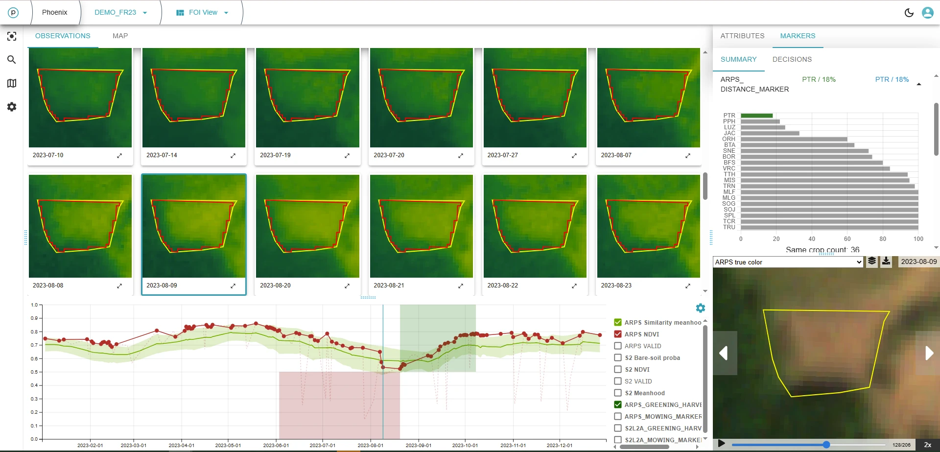
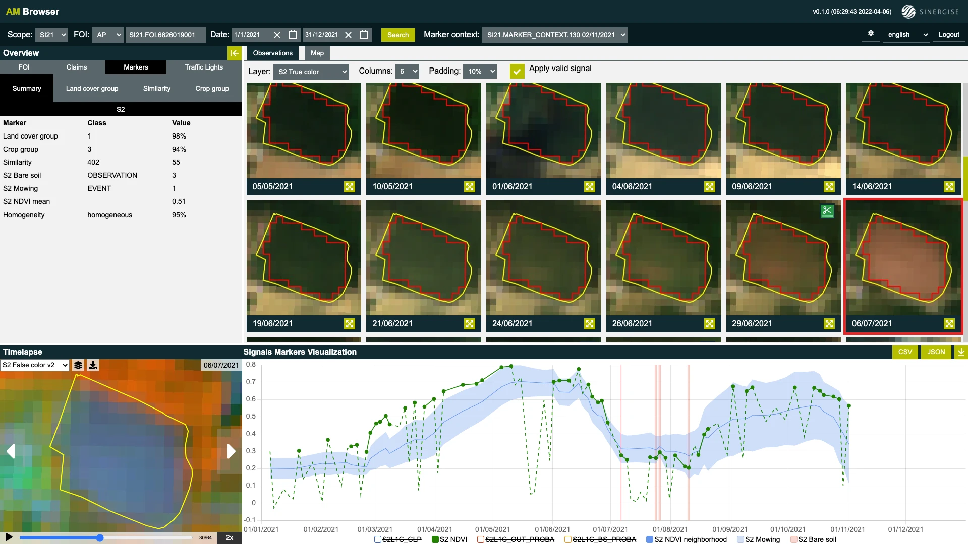
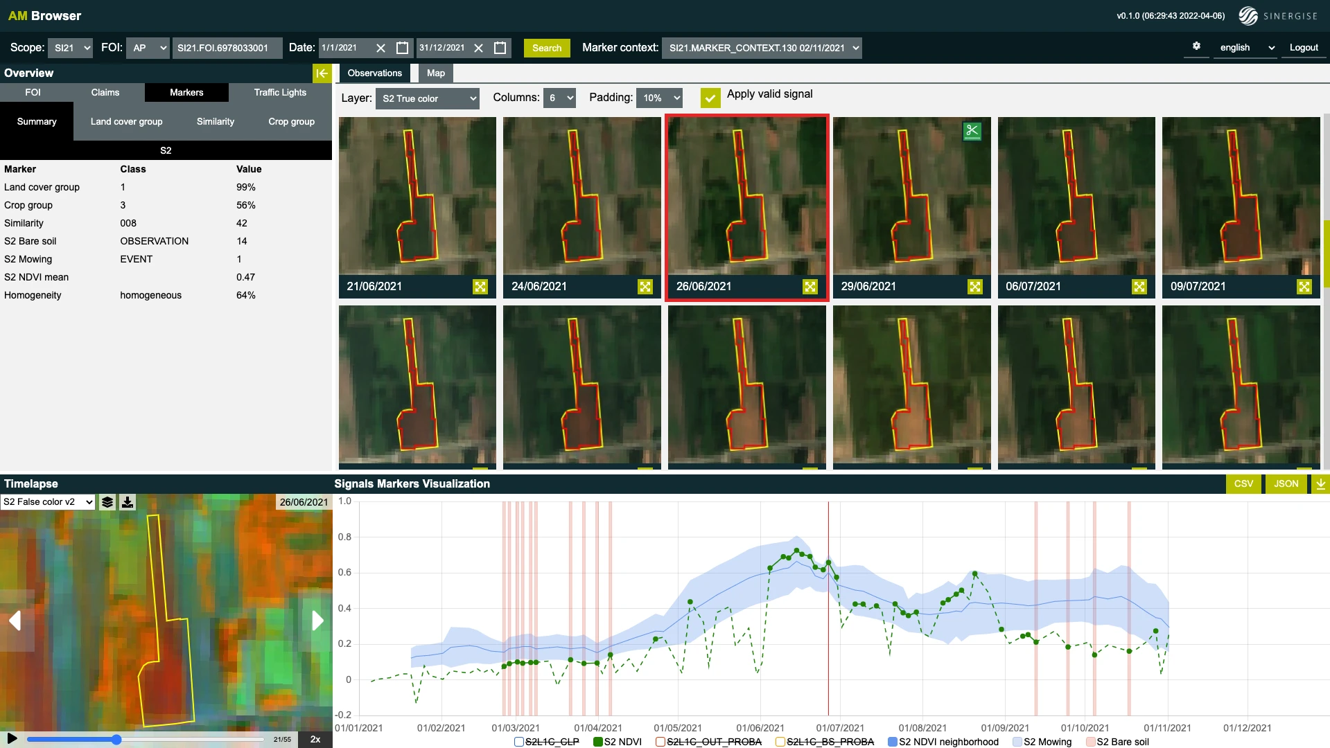
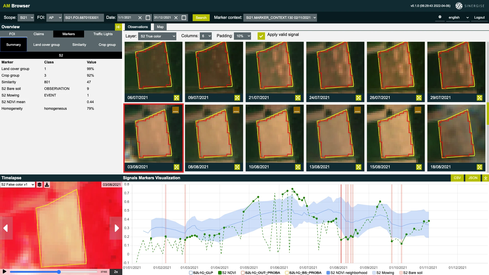
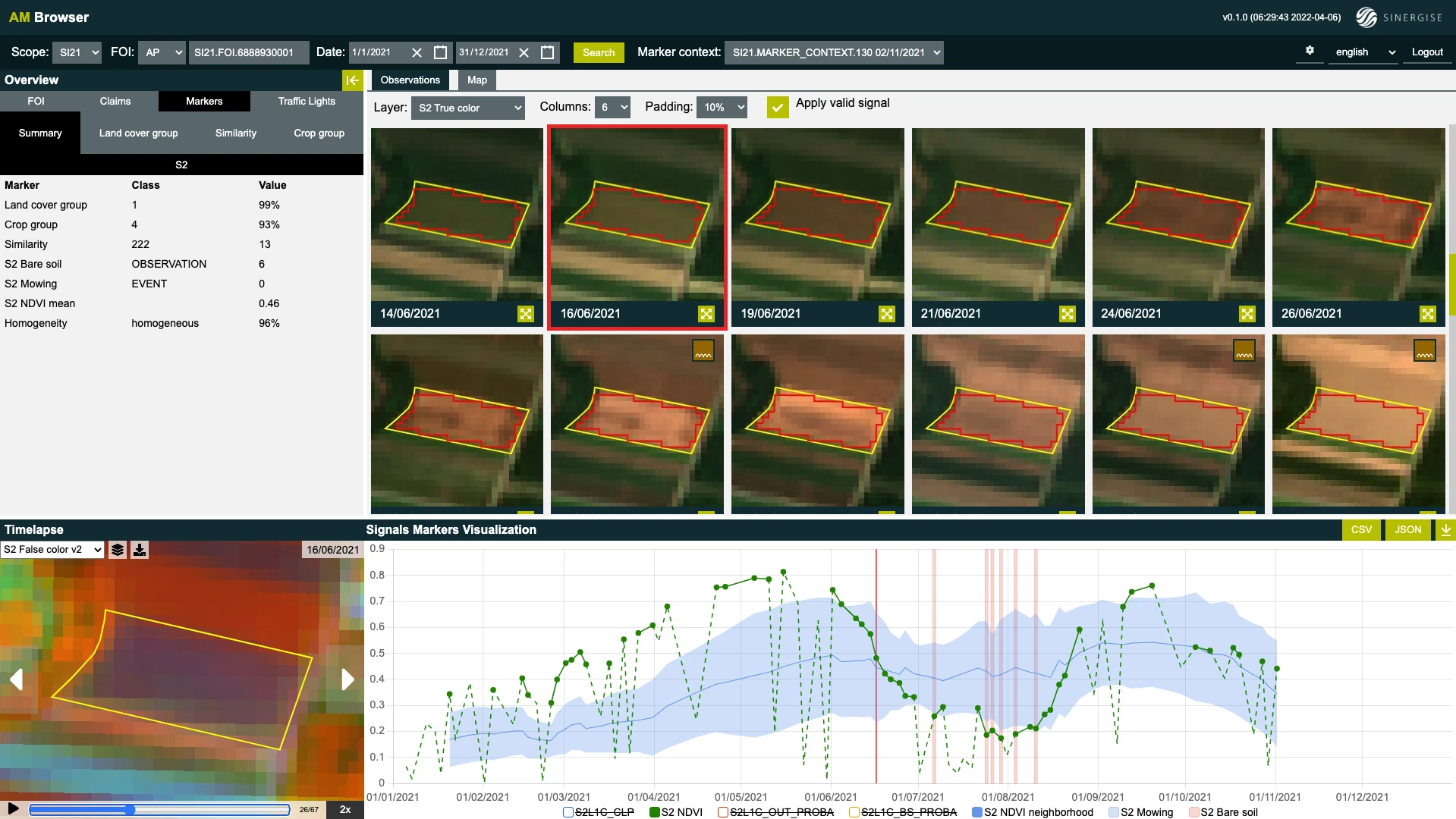
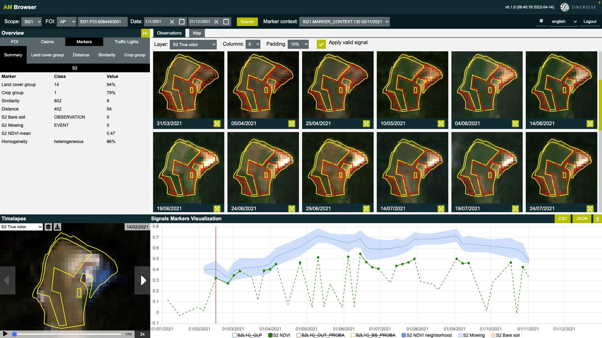
RapidEye\* Visual Product | RGB | RGB | Weekly
Monthly
Quarterly | 15 | MODIS | *\*RapidEye Imagery is used in Global Mosaics for dates before to February, 2020.* #### Normalized Surface Reflectance Mosaics **Normalized Surface Reflectance Mosaics** are created using the Ortho Analytic Surface Reflectance imagery asset type ([ortho\_analytic\_4b\_sr/ortho\_analytic\_8b\_sr](https://docs.planet.com/data/imagery/planetscope/psscene.md)). These mosaics are optimized to reduce the variability due to atmospheric effects, enabling users to perform spectral, quantitative, and time series analyses. Normalized Surface Reflectance Mosaics undergo additional processing steps to improve spatial and temporal consistency, making them less likely to have seamlines. The normalization process involves matching the mosaics to a common reference target. The targets are multi-year monthly composite mosaics, derived using Sentinel-2 imagery, with the goal of enhancing the spatial and temporal consistency of the mosaics, enabling time-series analyses. Nonetheless, the normalization process can result in less accurate absolute spectral values. These mosaics are ideal for use cases where spatial consistency is prioritized or for generating training data for machine learning algorithms. They are particularly suited for longer time periods (for example, monthly, quarterly) where multiple scenes are mosaicked together, and additional image processing is beneficial. Applications include land cover classification, forest disease monitoring, and flood risk analysis. #### Mosaics - Normalized Surface Reflectance source imagery | Source imagery | Download bands | Streaming bands | Monitoring frequency | Zoom level | Color target | | -------------------------------------- | --------------------------- | --------------- | ---------------------------------- | ---------- | ------------ | | PlanetScope Surface
Reflectance | BGRN | RGB, CIR | Weekly
Monthly
Quarterly | 15 | Sentinel-2 | | PlanetScope 8-Band Surface Reflectance | CB,B,G,GII,Y,R,
RE,NIR | RGB, CIR | Weekly
Monthly
Quarterly | 15 | Sentinel-2 | #### SuperRes Mosaics Visual Mosaics are optimized to minimize the effects of cloud cover, haze, and topographic variations. These mosaics are color-corrected and designed for human viewing and computer vision analytics, enabling users to monitor landscape and infrastructure changes over time and space. | Source Imagery | Download Bands | Streaming Bands | Frequency | Zoom Level | | -------------------------------------------------------------------------------------------------------- | -------------- | --------------- | ------------------------------------------------ | ---------- | | visual ortho\_analytic\_4b top of atmosphere reflectance and surface reflectance ortho\_analytic\_4b\_sr | RGB | RGB | Weekly
Biweekly
Monthly
Quarterly | 15 | \**SuperRes Mosaics general specifications* SuperRes Mosaics are created using the visual ortho\_analytic\_4b top of atmosphere reflectance imagery asset and the surface reflectance `ortho_analytic_4b_sr`. These mosaics are optimized to visually enhance human and machine perception of PlanetScope imagery. SuperRes Mosaics leverage our foundational model built on the Enhanced Super-Resolution Generative Adversarial Network (ESRGAN) with a collection of 120,000 pairs of SkySat and PlanetScope imagery with a perceptual loss training technique to produce imagery that looks natural and remains faithful to the ground truth. We include a confidence layer to help assess the degree of accuracy of the generated pixel by evaluating various sources of error. Learn more about our [SuperRes model’s specification and performance](https://docs.planet.com/data/imagery/superres/) on the product page. #### Mosaics - Normalized Surface Reflectance Product Details | Type | Prioritizes | Data | Pixel values | Normalization | | -------------------- | --------------------------------------------- | -------------- | ---------------------------- | ------------- | | Normalized SR | Spatial & temporal consistency; training data | 4-band, 16-bit | Modified Surface Reflectance | Sentinel-2 | | 8-Band Normalized SR | Spatial & temporal consistency; training data | 8-Band, 16-bit | Modified Surface Reflectance | Sentinel-2 | #### Mosaics - availability | Type | Available after | UDM2 | Pixel provenance | | -------------------- | --------------- | ----------------- | ---------------- | | Visual | January 2016 | Mixed | Yes | | Normalized SR | May 2016 | After August 2018 | Yes | | 8-Band Normalized SR | August 2020 | Yes | Yes | ## Product Specifications #### Mosaic quads Mosaics use the Web Mercator projection, the standard for web mapping applications, due to its efficiency in handling large geospatial datasets. This projection supports a tile-based system, dividing the world into uniform square tiles at multiple zoom levels. This allows for pre-rendered and cached tiles for fast map loading and smooth user interactions in GIS applications. Mosaics are distributed as a grid of GeoTIFF files, which are called *quads*—the size of each quad is 4096 x 4096 pixels. ![Web Mercator Tiling Grid with Monthly Visual Mosaic of Jamaica, April, 2024](/assets/images/jamaica_quads-32b4b80a2653c86a5f7b8e190c9ab857.webp "Web Mercator Tiling Grid with Monthly Visual Mosaic of Jamaica, April, 2024") *Web Mercator Tiling Grid with Monthly Visual Mosaic of Jamaica, April, 2024* | Attribute | Description | | --------------- | ------------------------------------------------------------------------------------------------------------------------------------------------------------------------------- | | Imagery | PlanetScope and RapidEye (Visual)
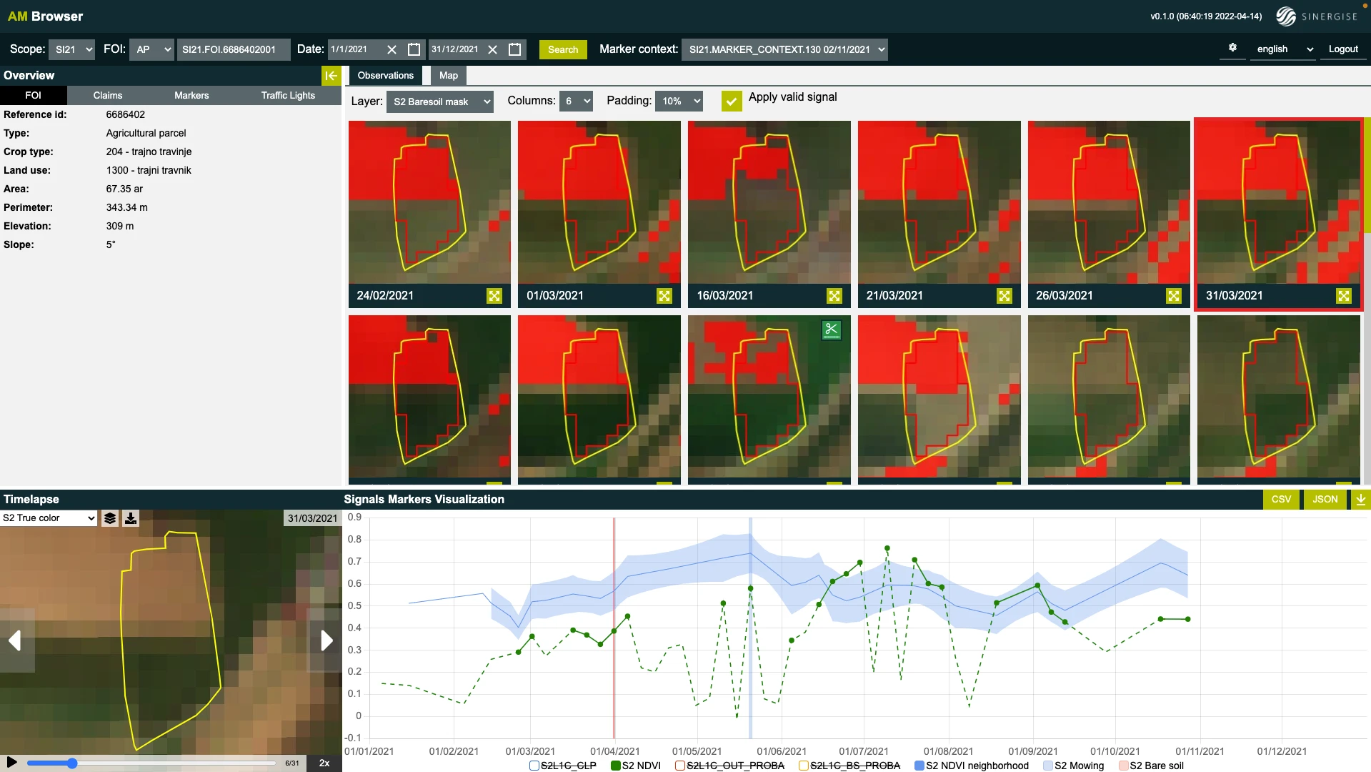
PlanetScope (Surface Reflectance) | | Pixel Size\* | 4.77 m at the Equator for zoom level 15 (PlanetScope and RapidEye) | | Image Bit Depth | 8-bit (Visual)
16-bit (Surface Reflectance) | | Bands | Red, Green, Blue, Alpha (Visual)
Blue, Green, Red, NIR, Alpha (Surface Reflectance)
Coastal Blue, Blue, Green I, Green II, Yellow, Red, Red Edge, NIR, Alpha (8 band) | | Projection | WGS84 Web Mercator (EPSG:3857) | | Size | 4096 x 4096 pixels | | Processing | Orthorectification
Atmospheric correction (Surface Reflectance only)
May be radiometrically balanced
Seamlines may be minimized with tonal balancing
| *\*The pixel size in meters can be estimated as follows: 4.77 \* cos(latitude) m (4.77 m at the Equator) for zoom level 15 (PlanetScope and RapidEye)*. #### Product naming The name of each mosaic quad represents the x and y position of the quad within the two-dimensional grid which makes up the mosaic. For example, `{X}-{Y}`, where X and Y are the x and y position of the quad in the grid. Example: `439-1220` Upon download, the name of the downloaded quad also contains the Zoom Level. Example: `L15-0439E-1220N.tif` #### Publication Planet aims to publish all Mosaics 7 days after the end of the acquisition period. However, there may be instances where publishing may take longer. Publishing times for custom mosaics are determined on a case-by-case basis. #### Cadence Mosaics are generated at a specified cadence based on the `first_acquired` and `last_acquired` UTC timestamps for underlying source imagery. | Cadence | Start (`first_acquired`) | End (`last_acquired`) | | --------- | ----------------------------------------------------------------- | ------------------------------------------------------------------------ | | Weekly | Mondays at 00:00:00 UTC | Sundays at 23:59:59 UTC | | Monthly | The first day of each month at 00:00:00 UTC | The last day of each month at 23:59:59 UTC | | Quarterly | January 1st, April 1st, July 1st, and October 1st at 00:00:00 UTC | March 31st, June 30th, September 30th, and December 31st at 23:59:59 UTC | ## Mosaics Delivery Mosaics can be downloaded or streamed through multiple methods. Below are some of the available options. ### Planet Insights Platform [Planet Insights Platform](https://insights.planet.com/data/mosaics) can be used to view and download mosaic quads. A complete tutorial on how to use the Planet Insights Platform to access Mosaics is available in this [introductory course](https://university.planet.com/introduction-to-planet-basemaps) from Planet University. ### QGIS/ArcGIS Pro plugins Mosaics can be downloaded or streamed through the Planet [QGIS](https://docs.planet.com/platform/integrations/qgis/planet-qgis-plugin.md#explore-basemaps) or [ArcGIS Pro](https://docs.planet.com/platform/integrations/arcgis/planet-add-in-for-arcgis-pro.md#explore-basemaps) plugins. These plugins enable users to search for mosaics within the catalog and offer multiple filtering options, such as filtering by area of interest or by different types of mosaics. ### Orders API Mosaics can also be accessed through the Orders API, which allows users to reproject the data to a coordinate system other than Web Mercator, clip mosaics to a specified extent, merge multiple quads, perform band math calculations, and deliver the data to a cloud service provider. However, there are limitations to consider. Users can merge and download up to 25 quads at once. If the merge tool is not used, the limit is 500 quads per order, meaning the provided geometry must encompass fewer than 500 quads. For downloading areas larger than 500 quads, it is recommended to use the Basemaps API. For more detailed information, see [the Mosaics documentation](https://docs.planet.com/develop/apis/orders/sources.md#mosaics-source-type). ### Basemaps API The Basemaps API is recommended for users seeking endpoints for scalable workflows, direct access to Cloud Optimized GeoTIFF links, and the ability to stream mosaics into web applications. Often, users combine the capabilities of both APIs (Orders and Basemaps) when writing their own libraries to access mosaics. The detailed API reference can be found [here](https://docs.planet.com/develop/apis/basemaps/reference.md). Some use cases of the Basemaps API are: * Find the quads that intersect an Area of Interest and download those quads. * Get the list of items that contribute to the particular quad. * Stream into web applications using the XYZ and WMTS protocols. * Get a list of series and mosaics available for a user. ### Tile Services Planet's Mosaic WMTS and XYZ tile services provide programmatic streaming access to Mosaics including full bit depth data. ### Quad Packaging Mosaic quads can be downloaded through the Basemaps API and Orders API along with their associated metadata (JSON), [UDM2](https://docs.planet.com/data/imagery/udm.md) assets, and pixel provenance raster and vector files, which trace all scenes used when producing the quads. The table below shows the list of files returned when downloading a single quad, and their associated files, for a Normalized SR Mosaic. | File name | Size | | -------------------------------- | ------ | | 484-1310\_quad.tif | 117 MB | | 484-1310\_provenance\_raster.tif | 236 KB | | 484-1310\_ortho\_udm2.tif | 1.2 MB | | 484-1310\_provenance\_vector.zip | 22 KB | | L15-0484E-1310N.dbf | 788 B | | L15-0484E-1310N.prj | 425 B | | L15-0484E-1310N.shp | 66 KB | | L15-0484E-1310N.shx | 124 B | --- Copy for LLM[View as Markdown](https://docs.planet.com/data/imagery/mosaics/sandbox/) # Planet Mosaics Sandbox Data This Planet Sandbox Data collection for Planet Mosaics provides sample data over specific areas and times of interest. The data is available to paid and trial accounts that include processing units and is available under the CC-BY-NC license. Learn more about [Planet Sandbox Data](https://docs.planet.com/data/planet-sandbox-data.md). ## Data Collections Metadata | Source ID | Collection Name | Collection ID | Time Range | | --------------------------------------- | -------------------------------------------- | ----------------------------------------- | ----------------------- | | ps\_s2\_normalized\_sr\_monthly\_mosaic | Planet Sandbox Data - Planet Monthly Mosaics | BYOC-c48c018f-67a1-4827-a1e4-f3ab98690312 | 2021-01-01 - 2023-04-01 | ## Planet Sandbox Data Areas This collection includes 9 sandbox regions. Download the GeoJSON file below the map for exact polygon boundaries. View all 9 regions | Location | Area (km²) | Time Range | Center (lat, lon) | | ----------------------------------------------- | ---------- | ----------------------- | ----------------- | | Cusco, Province of Chumbivilcas, Peru | 3211 | 2021-01-01 – 2023-04-01 | -14.52, -71.81 | | Iowa, United States | 28229 | 2021-01-01 – 2023-04-01 | 41.11, -93.78 | | Mato Grosso, Central-West Region, Brazil | 1445 | 2021-01-01 – 2023-04-01 | -13.07, -56.60 | | Pará, North Region, Brazil | 27021 | 2021-01-01 – 2023-04-01 | -6.66, -52.29 | | Nouvelle-Aquitaine, Metropolitan France, France | 19181 | 2021-01-01 – 2023-04-01 | 44.65, -0.44 | | Svalbard, Norway | 97 | 2021-03-01 – 2023-04-01 | 78.17, 15.56 | | Dodoma Region, Central Zone, Tanzania | 2255 | 2021-01-01 – 2023-04-01 | -6.32, 36.83 | | Al Qalyubiya, Egypt | 13962 | 2021-01-01 – 2023-04-01 | 30.22, 31.20 | | Western Australia, Australia | 29827 | 2021-01-01 – 2023-04-01 | -31.72, 116.54 | [Download GeoJSON](https://docs.planet.com/data/imagery/mosaics/polygons.geojson) ## Highlights [![São Félix do Xingu, Brazil](/data/imagery/mosaics/PB_BRA.webp)](https://insights.planet.com/analyze/browser/?zoom=9\&lat=-6.7652\&lng=-52.3763\&themeId=PLANET_SANDBOX\&visualizationUrl=https%3A%2F%2Fservices.sentinel-hub.com%2Fogc%2Fwms%2F64e8174f-7d03-4863-ba70-5139e325a75d\&datasetId=c48c018f-67a1-4827-a1e4-f3ab98690312\&fromTime=2023-04-01T00%3A00%3A00.000Z\&toTime=2023-04-01T23%3A59%3A59.999Z\&layerId=TRUE-COLOR\&demSource3D=%22MAPZEN%22) São Félix do Xingu, Brazil 2021-01-01 to 2023-04-01
27021km² [Visualize in the Browser →](https://insights.planet.com/analyze/browser/?zoom=9\&lat=-6.7652\&lng=-52.3763\&themeId=PLANET_SANDBOX\&visualizationUrl=https%3A%2F%2Fservices.sentinel-hub.com%2Fogc%2Fwms%2F64e8174f-7d03-4863-ba70-5139e325a75d\&datasetId=c48c018f-67a1-4827-a1e4-f3ab98690312\&fromTime=2023-04-01T00%3A00%3A00.000Z\&toTime=2023-04-01T23%3A59%3A59.999Z\&layerId=TRUE-COLOR\&demSource3D=%22MAPZEN%22) [![Bordeaux, France](/data/imagery/mosaics/PB_FRA.webp)](https://insights.planet.com/analyze/browser/?zoom=9\&lat=44.7345\&lng=-0.676\&themeId=PLANET_SANDBOX\&visualizationUrl=https%3A%2F%2Fservices.sentinel-hub.com%2Fogc%2Fwms%2F64e8174f-7d03-4863-ba70-5139e325a75d\&datasetId=c48c018f-67a1-4827-a1e4-f3ab98690312\&fromTime=2023-04-01T00%3A00%3A00.000Z\&toTime=2023-04-01T23%3A59%3A59.999Z\&layerId=TRUE-COLOR\&demSource3D=%22MAPZEN%22) Bordeaux, France 2021-01-01 to 2023-04-01
19181km² [Visualize in the Browser →](https://insights.planet.com/analyze/browser/?zoom=9\&lat=44.7345\&lng=-0.676\&themeId=PLANET_SANDBOX\&visualizationUrl=https%3A%2F%2Fservices.sentinel-hub.com%2Fogc%2Fwms%2F64e8174f-7d03-4863-ba70-5139e325a75d\&datasetId=c48c018f-67a1-4827-a1e4-f3ab98690312\&fromTime=2023-04-01T00%3A00%3A00.000Z\&toTime=2023-04-01T23%3A59%3A59.999Z\&layerId=TRUE-COLOR\&demSource3D=%22MAPZEN%22) [![Perth, Australia](/data/imagery/mosaics/PB_AUS.webp)](https://insights.planet.com/analyze/browser/?zoom=9\&lat=-31.702\&lng=116.524\&themeId=PLANET_SANDBOX\&visualizationUrl=https%3A%2F%2Fservices.sentinel-hub.com%2Fogc%2Fwms%2F64e8174f-7d03-4863-ba70-5139e325a75d\&datasetId=c48c018f-67a1-4827-a1e4-f3ab98690312\&fromTime=2023-04-01T00%3A00%3A00.000Z\&toTime=2023-04-01T23%3A59%3A59.999Z\&layerId=TRUE-COLOR\&demSource3D=%22MAPZEN%22) Perth, Australia 2021-01-01 to 2023-04-01
29827km² [Visualize in the Browser →](https://insights.planet.com/analyze/browser/?zoom=9\&lat=-31.702\&lng=116.524\&themeId=PLANET_SANDBOX\&visualizationUrl=https%3A%2F%2Fservices.sentinel-hub.com%2Fogc%2Fwms%2F64e8174f-7d03-4863-ba70-5139e325a75d\&datasetId=c48c018f-67a1-4827-a1e4-f3ab98690312\&fromTime=2023-04-01T00%3A00%3A00.000Z\&toTime=2023-04-01T23%3A59%3A59.999Z\&layerId=TRUE-COLOR\&demSource3D=%22MAPZEN%22) --- Copy for LLM[View as Markdown](https://docs.planet.com/data/imagery/mosaics/surfacereflectance/) # Surface Reflectance Mosaics ![Header Thumbnail](/data/imagery/mosaics/cir.webp) Mosaics are generated by querying scenes that overlap a specific area of interest within a designated time frame. These scenes are then ranked based on quality metrics metadata, such as the presence of clouds and haze, with the highest quality scenes placed at the top. Using a best-on-top algorithm, the highest quality scenes are efficiently composited to create the final mosaic. **Normalized Surface Reflectance Mosaics** (Zoom Level 15 – 4.77 meter cell size at the equator) are created using the Ortho Analytic Surface Reflectance imagery asset type ([ortho\_analytic\_4b\_sr/ortho\_analytic\_8b\_sr](https://docs.planet.com/data/imagery/planetscope/psscene.md) ). These mosaics are optimized to reduce the variability due to atmospheric effects, enabling users to perform spectral, quantitative, and time series analyses. For more details, see the [Mosaics Webpage](https://docs.planet.com/data/imagery/mosaics.md) and the [Mosaic Product Technical Specification](https://assets.planet.com/products/basemap/planet-basemaps-product-specifications.pdf) document. ### Normalized Surface Reflectance Mosaics Product Details | Source imagery | Download bands | Streaming bands | Monitoring frequency | Zoom level | Color target | | -------------------------------------------------- | -------------- | --------------- | ---------------------------------- | ---------- | ------------------------------------- | | PlanetScope Surface Reflectance
`analytic_sr` | BGRN | RBG, CIR | Weekly
Monthly
Quarterly | 15 | Sentinel-2
None (non-normalized) | --- Copy for LLM[View as Markdown](https://docs.planet.com/data/imagery/mosaics/techspec/) # Technical Specification ### Download the PDF [Download PlanetScope Mosaics Imagery Product Specification →](https://planet.widen.net/view/pdf/gbkcexll3p/Planet-UserDocumentation-MosaicsProductSpecification.pdf) --- Copy for LLM[View as Markdown](https://docs.planet.com/data/imagery/mosaics/visual/) # Visual Mosaics ![Header Thumbnail](/data/imagery/mosaics/visual.webp) PlanetScope Mosaics are generated by querying PlanetScope scenes that overlap a specific area of interest within a designated time frame. These scenes are then ranked based on quality metrics metadata, such as the presence of clouds and haze, with the highest quality scenes placed at the top. Using a best-on-top algorithm, the highest quality scenes are efficiently composited to create the final mosaic. **PlanetScope Visual Mosaics** (Zoom Level 15 – 4.77 meter cell size at the equator) are optimized to minimize the effects of cloud cover, haze, and topographic variations. These mosaics are generated using the [visual](https://docs.planet.com/data/imagery/planetscope/psscene.md) asset type, and are color-corrected and designed for human viewing and computer vision analytics, enabling users to monitor landscape and infrastructure changes over time and space. **SkySat Visual Mosaics** (Zoom Level 18 – 0.596 meter cell size at the equator) can be generated post SkySat tasking over a custom area and time of interest. SkySat Visual Mosaics are generated using [ortho\_visual](https://docs.planet.com/data/imagery/skysat/item-types/skysatcollect.md) asset type. In addition, SkySat Visual Mosaics may be purchased as an add-on to our Flexible Tasking product. For more details, see the [Mosaics Webpage](https://docs.planet.com/data/imagery/mosaics.md) and the [Mosaic Product Technical Specification](https://assets.planet.com/products/basemap/planet-basemaps-product-specifications.pdf) document. ### Visual Mosaics Product Details | Source imagery | Download bands | Streaming bands | Monitoring frequency | Zoom level | Color target | | --------------------------------------------------------------------- | -------------- | --------------- | ---------------------------------------------- | ---------- | ------------------------------------------------------------ | | PlanetScope and/or
RapidEye\* Visual Product
`visual` asset | RGB | RGB | Weekly
Monthly
Quarterly | 15 | MODIS | | SkySat Visual Product
`ortho_visual` asset | RGB | RGB | Weekly
Monthly
Quarterly
Custom | 18 | PlanetScope (normalized to MODIS)
None (non-normalized) | *\*RapidEye Imagery is used in Global Mosaics for dates prior to February 2020.* --- Copy for LLM[View as Markdown](https://docs.planet.com/data/imagery/pelican/) ![Header Thumbnail](/data/imagery/pelican/thumbnail.webp) # Pelican Overview ## Constellation & Sensor Overview Pelican, operated by Planet, is a next-generation high-resolution constellation designed to support rapid tasking, improved image quality, and low-latency delivery. Pelican produces multispectral and panchromatic imagery and is sampled at **50 centimeters per pixel** when orthorectified. The Pelican satellite constellation consists of multiple launches of Generation-1 Pelican spacecraft, beginning commercial operations in 2025. Each satellite is **3-axis stabilized** and highly agile, capable of slewing rapidly between targets of interest. Pelican satellites include an electric propulsion unit for orbital control, along with **four reaction wheels and three magnetic torquers** for attitude control. Generation-2 spacecraft are anticipated to begin operations in 2026. Pelican supports multiple collection modes including point, line, area, and developing stereo capabilities. Pelican captures imagery as continuous strips that are segmented into framed Scenes. Pelican Gen-1 collects an **8 km swath** at nadir. Pelican Gen-1 satellites contain high-performance **Cassegrain telescopes** with an effective focal length of **4.03 meters**, paired with a line-scan detector system consisting of **dual panchromatic sensor arrays (12,288 pixels)** and **six multispectral bands (6,144 pixels)**. The panchromatic sensors are diagonally offset by half a pixel, enabling oversampling used in advanced processing and pansharpening. Pelican collects imagery in 6 multispectral bands alongside the panchromatic channel. Pelican imagery is captured using **Time Delay Integration (TDI)**, enabling high SNR at high resolution. The multispectral pixels have a larger native sample distance, while the panchromatic band provides finer detail for pansharpened and visual products. Pelican collects frame imagery in all tasking modes and is engineered for fast downlink and rapid product availability. ### Pelican Spectral Bands Pelican satellites have two spectral band configurations: **Pelican-2** and **Generation-1 Pelican (Pelican-3 through Pelican-10)**. The table below presents both sets of bands side-by-side for easy comparison. Pelican Generation 2 satellites will have the same band configurations as Generation 1. | **Band** | **Pelican-2 (nm)** | **Gen-1 and Gen-2 Pelicans (nm)
(Pelican-3+)** | | ------------------- | ------------------ | --------------------------------------------------- | | **Panchromatic** | 450 – 800 | 450 – 800 | | **Blue** | 450 – 520 | 465 – 518 | | **Green** | 520 – 590 | 547 – 585 | | **Red** | 630 – 690 | 650 – 682 | | **Red Edge / RE-I** | 693 – 715 | 699 – 716 | | **Red Edge II** | 729 – 751 | — | | **NIR** | 770 – 890 | — | | **NIR Wide** | — | 779 – 885 | | **NIR Narrow** | — | 846 – 887 | ## Pelican Imagery Products Pelican products are available for search and download via the Planet APIs, User Interfaces, and integrations. Pelican imagery is delivered in the form of **Scene products**, which are encoded in the Planet Platform as a set of Item Types and Asset Types. All Pelican imagery is collected as continuous strips using a line-scan sensor and then segmented into framed Scenes for processing and delivery. Pelican supports **multiple radiometric and geometric processing levels**, including Level 1A (minimally processed panchromatic), Level 1B Basic (radiometrically and sensor-corrected), and Level 3B Ortho (fully orthorectified radiance, surface reflectance, pansharpened, and visual products). These products are interoperable with Planet’s high-resolution SkySat offerings while improving upon image quality, artifact reduction, and delivery speed. ### Item Types A **Pelican Scene Product** is an individual framed segment extracted from a Pelican imaging strip. Each strip is captured with a dual-panchromatic + multispectral line-scan system and then divided into Scenes for processing. Pelican Scenes typically cover an **8 km swath width** and vary in length depending on the tasking mode and imaging geometry. Pelican Scenes are represented in the Planet Platform as the `PelicanScene` item type. Each Scene includes: * Panchromatic and multispectral imagery * Geometry footprint and acquisition metadata * UDM2 (Usable Data Mask) for cloud, haze, shadow, snow/ice, and unusable pixels * RPC files for Basic products * Projection and radiometric metadata for Ortho products Pelican does **not** include a Collect product type, equivalent to SkySatCollect, as PelicanScenes do not require scene to scene mosaic as SkySatScenes do. ### Imagery Asset Types Pelican Scene products are available for download in the form of imagery assets. Multiple asset types are made available for Pelican Scenes, each with differences in radiometric processing, geometric correction, and spectral content. Asset type availability varies by processing level. **Basic L1A Panchromatic** (`basic_l1a_panchromatic`) assets are minimally processed, non-orthorectified panchromatic imagery products. These products include raw-mapped detector values with accompanying calibration coefficients and are designed for advanced users requiring earliest access or custom radiometric workflows. **Basic Panchromatic** (`basic_panchromatic`) assets are non-orthorectified, calibrated panchromatic imagery products. They include Time Delay Integration (TDI) corrections and are transformed to scaled Top of Atmosphere Radiance. These products are designed for data science and analytic workflows that benefit from Pelican’s wide (450–800 nm) panchromatic band and include associated rational polynomial coefficients (RPCs) for user-driven orthorectification. **Basic Analytic** (`basic_analytic`) assets are non-orthorectified, calibrated multispectral imagery products. They contain Pelican’s six spectral bands at native multispectral resolution and are transformed to scaled Top of Atmosphere Radiance. These products are intended for analytic applications requiring spectral fidelity and for users who wish to geometrically correct the imagery themselves using RPCs. **Ortho Panchromatic** (`ortho_panchromatic`) assets are orthorectified, calibrated panchromatic imagery products resampled to a uniform 50 cm pixel size. These products provide high-resolution detail suitable for geospatial analysis, mapping, and applications requiring accurate cartographic projection. **Ortho Analytic** (`ortho_analytic`) assets are orthorectified, calibrated 6-band multispectral imagery products transformed to Top of Atmosphere Radiance and delivered at a 1 m pixel size. They are intended for workflows requiring accurate geolocation and multispectral analysis. **Ortho Analytic Surface Reflectance** (`ortho_analytic_sr`) assets are orthorectified 6-band multispectral imagery corrected for the effects of the Earth’s atmosphere, accounting for the molecular composition and variation with altitude along with aerosol content. Combining the use of standard atmospheric models with the use of MODIS or VIIRS for water vapor, ozone and aerosol data, this provides reliable and consistent surface reflectance scenes over Planet’s varied constellation of satellites as part of our normal, on-demand data pipeline. **Ortho Pansharpened** (`ortho_pansharpened`) assets are orthorectified 6-band multispectral imagery sharpened using Pelican’s oversampled dual-panchromatic channels to achieve 50 cm resolution. These products are designed for multispectral applications requiring the highest available spatial detail combined with spectral richness. **Ortho Visual** (`ortho_visual`) assets are orthorectified, color-corrected RGB imagery optimized for visualization. Lower-resolution multispectral bands are pansharpened to 50 cm using Pelican’s dual-panchromatic imagery. These products are intended for direct visual inspection and easy ingestion into GIS platforms. **UDM2** (`*_udm2`) assets are Usable Data Masks accompanying both Basic and Ortho products. UDM2 identifies clear, cloud, haze, shadow, snow/ice, confidence, and unusable pixels, enabling users to filter or mask portions of the Scene. Pelican’s full product specifications can be found in the [Pelican User Documentation](https://planet.widen.net/s/kbt9m6p6sx/planet-userdocumentation-pelicanproductspec). ## Product Naming Pelican image products follow two naming conventions depending on whether the file is a **full Scene** or a **trimmed deliverable** produced as part of task fulfillment. Both conventions provide globally unique identifiers for acquisition time, satellite, and asset type. ### Full Scene Image Filename Convention Full Pelican Scene products use the following naming pattern: ``` ___. ``` Examples: ``` 20250305_143613_03_3009_Analytic.tif 20250305_143613_03_3009_Visual.tif ``` This convention applies to all complete Pelican Scenes generated directly from the imaging strip before trimming or task‑specific processing. ### Trimmed Imagery Folder Naming Convention Trimmed assets, delivered for task fulfillment, include an additional **unique capture identifier** in the folder name: ``` ___ ``` Example: ``` 20250305_143613_03_3009_3a44e78a-de6d-4d4b-b199-8f142deb10dd ``` ## Processing Several processing steps are applied to Pelican imagery to produce the complete set of Pelican Scene products available for download. ![High Resolution Processing Chain illustration](/assets/images/Graphics_for_High_Res_Processing_Chain-c8f0f071d833ff9fc144bca8fd198a4b.webp) ### Sensor & Radiometric Calibration ### *Sensor* **Darkfield/Offset Correction**: Corrects for sensor bias and dark noise. On-orbit calibration collects are captured with the same operational settings during eclipse to yield faithful representative darkfield images. Darkfield images are updated periodically for all bands. **Flat Field Correction:** Flat fields are created from on-orbit imagery taken post-launch. These fields are used to correct sensor non-uniformities. Flat field images are updated periodically for all bands. **Band Co‑Registration**: Aligns Pelican’s dual panchromatic channels and six multispectral bands using an improved geometric model, ensuring pixel‑accurate spectral alignment across the stack. ### *Radiometric* **Absolute Radiometric Calibration**: Converts detector digital number (DN) measurements into physical radiance units (W/(m²·sr·µm)) using calibration coefficients derived from laboratory and on‑orbit calibration. **Atmospheric Correction**: Surface reflectance is determined from Top of Atmosphere (TOA) reflectance, calculated using coefficients supplied with the Planet Radiance product. The Planet Surface Reflectance product corrects for the effects of the Earth's atmosphere, accounting for the molecular composition and variation with altitude along with aerosol content. Combining the use of standard atmospheric models with the use of satellite water vapor, ozone and aerosol data, this provides reliable and consistent surface reflectance scenes over Planet's varied constellations of satellites as part of our normal, on-demand data pipeline. However, there are some limitations to the corrections performed: * In some instances, there is no satellite data overlapping a Planet scene or the area nearby. In those cases, AOD is set to a value of 0.226 which corresponds to a “clear sky” visibility of 23 km, the aot\_quality is set to the satellite “no data” value of 127, and aot\_status is set to ‘Missing Data - Using Default AOT’. If there is no overlapping water vapor or ozone data, the correction falls back to a predefined 6SV internal model. * The effects of haze and thin cirrus clouds are not corrected for. * Aerosol type is limited to a single, global model. * All scenes are assumed to be at sea level, and the surfaces are assumed to exhibit Lambertian scattering - no BRDF effects are accounted for. * Stray light and adjacency effects are not corrected for. ### *Visual* ### Visual Product Processing Pelican Visual products present imagery as natural color, optimized for human interpretation. Processing includes: 1. **Color Curve Application**: A custom color profile is applied to enhance visual clarity and alignment with natural appearance. 2. **Pansharpening**: Lower‑resolution multispectral bands are fused with Pelican's dual‑panchromatic channels to produce a 50 cm RGB product. 3. **Post‑Processing Enhancements**: Final tuning steps to ensure consistent tone and contrast across the continuous sequence of images captured by the satellite during a single pass over an area. We do not guarantee visual consistency between non-continuous sequences of images, nor across independent passes over an area. ### Geometric Processing Pelican imagery undergoes a multistep georectification process to ensure positional and geometric accuracy meets Planet’s quality standards. This process transforms the raw satellite imagery into a map-ready product. Planet image products are offered with different levels of processing to correct for sensor and geometric distortions which include the following product levels: * **Basic Products:** These are sensor-corrected and geometrically aligned. Basic products are georeferenced to improve positional accuracy beyond what telemetry alone provides, but they are not orthorectified or corrected for terrain distortions. * **Ortho Products:** In addition to the corrections applied to Basic products, Ortho products account for terrain distortion. Imagery is orthorectified and projected onto a 50 cm grid using a digital elevation model (DEM) to accurately model local terrain. Ortho products utilize the UTM WGS84 map projection #### Geometric Processing Workflow Both Basic and Ortho products are generated from a rigorous sensor model refined through these steps: 1. **Initial Pointing Estimate:** Satellite telemetry provides the initial pointing estimate (typically 75–100 m accuracy). Corrections for boresight and optical distortion are applied within a physical camera model. 2. **Refined Pointing with Global Reference:** Ground control tie points from the panchromatic band are matched against global reference imagery. This refines the satellite attitude and corrects low‑frequency satellite motions. 3. **Band Alignment and Fine Refinement:** The remaining panchromatic and multispectral bands are rectified to the initial panchromatic band. This spatially aligns the bands and further refines the camera's attitude, removing higher-frequency satellite motions. After refinement, the updated physical camera model is used to generate final outputs: * **Basic Products:** Bands are aligned within the image plane. **Rational Polynomial Coefficients (RPCs)** are included for users who want to perform their own orthorectification. RPCs approximate the full camera model but may not be continuous across adjacent tiles. * **Ortho Scene Products:** Imagery is projected and resampled onto a fixed 50 cm grid using the refined camera model and a reference DEM. #### Geometric Processing Accuracy The positional accuracy of Planet imagery is contingent upon the efficacy of our multi-step georectification process. Variations in image characteristics and the availability of geodetic control influence the final geospatial accuracy. **Positional Accuracy in the Absence of Ground Control** Imagery acquired under conditions that preclude the extraction of sufficient ground control tie points (GCPs) will exhibit increased positional uncertainty. In such cases, the rigorous physical camera model will necessarily revert to parameter estimations derived predominantly from the initial satellite telemetry data. This results in a nominal absolute geospatial accuracy of 75 to 100 meters circular error 90% (CE90). Conditions contributing to this scenario include, but are not limited to: * **Significant cloud obscuration:** Extensive cloud cover prevents line-of-sight to ground features essential for GCP extraction. * **Dominant water bodies:** Large water features within a scene lack stable, distinct, and identifiable georeferencing points. * **Dynamic or homogenous terrain:** Regions undergoing rapid geomorphological change, or those characterized by uniform, featureless surfaces (for example, snow-covered expanses), impede reliable GCP generation. * Imagery relying solely on telemetry-derived positional estimates can be identified in the product metadata where the "Ground Control" field will be explicitly set to "FALSE". **Influence of Reference Data Fidelity** The absolute geospatial accuracy of Planet's derived image products is directly impacted by the inherent accuracy of the global reference imagery datasets utilized in our georectification pipeline. Specific details regarding the absolute accuracy of the reference data are systematically reported in Planet's quarterly Image Quality Reports (IQRs). For example, during Q1 through Q2, Planet's primary reference imagery demonstrated an absolute accuracy of 5 meters CE90 across the majority of locations characterized by terrain slopes less than 20 degrees. This CE90 metric signifies that 90% of the measured horizontal errors are expected to be within a 5-meter radius of the true ground position. Users may observe a localized degradation in absolute positional accuracy in geographic regions exhibiting: * **Rapid Urban Development or Significant New Construction:** Recent anthropogenic modifications may not be fully represented in the current reference data. * **Pronounced Topographical Changes:** Areas with dynamic geomorphic processes (for example, landslides, erosion) can lead to discrepancies. * **High Terrain Slopes:** Steep slopes inherently introduce greater geometric distortion and can challenge precise orthorectification, potentially reducing positional accuracy even with an accurate digital elevation model (DEM). Planet updates **reference data** to mitigate these factors and maintain optimal geospatial processing fidelity. The current DEM and reference imagery accuracy used for orthorectification is detailed in the relevant Image Quality Reports. ## Miscellaneous **Rational Polynomial Coefficients (RPCS)** For Pelican Basic Imagery, Planet supplies Rational Polynomial Coefficients (RPCs) similar to SkySat and PlanetScope. RPCs provide a mathematical relationship that maps the 3D ground coordinates (latitude, longitude, elevation) to 2D image coordinates (row, column pixels) and vice-versa. This is essential for accurately geolocating features within an image and for removing geometric distortions caused by sensor geometry, terrain variations, and satellite attitude during image acquisition. RPCs are ratios of polynomials that approximate a physical sensor model. They consist of a set of coefficients (numerators and denominators) for both forward (ground to image) and inverse (image to ground) transformations. These coefficients are derived as part of the Geometric processing. The RPCs are an approximation to a rigorous physical sensor model that Planet uses to generate Pelican Orthorectified image products. As such, users who use RPCs may find that their generated ortho image does not match Planet’s orthorectified imagery exactly. Currently, the RPCs are generated for individual tiles and discontinuities in the solution may occur at tile boundaries. RPCs are supplied with Basic products and designed for users with advanced image processing and geometric correction capabilities. Basic products are not orthorectified or corrected for terrain distortions by Planet. With accompanying RPC files users can perform these corrections themselves using standard GIS tools. Users will need an elevation model (for example, a Digital Elevation Model) to correctly orthorectify this product. For Pelican, the RPC files are supplied as text (.TXT) files. The following table describes the RPC file format. The RPCs are also available in the Tiff header for the Basic product. **Pelican NITF 2.1 Image Product** Planet can produce imagery in the National Imagery Transmission Format (NITF 2.1) compliant with MIL-STD-2500C and guidelines provided by the United States National Geospatial Intelligence Agency (NGA). The NITF provided for Pelican imagery includes the image itself, meta data, and the UDM mask. It includes a generic linear array scanner (GLAS) model in a standard format which allows for users to create orthorectified products from the imagery using a digital elevation model. The GFM is an approximation to the full physical model used by Planet. More information on the GLAS can be found in Theiss, ISPRS Annals of the Photogrammetry, Remote Sensing and Spatial Information Sciences, Volume V-1-2020. Full information on the MIL-STD-2500C standards is available through the United States NITF Technical board. NITF for Pelican implements a Generic Linear Array Scanner (GLAS) as its geometric sensor model because Pelican is a linear scanner. As such, Pelican produces a long continuous image which we segment into chunks, rather than a mosaic of images. Further, GLAS is a generic physical sensor model that applies to images that retain their original perspective geometry and have not been warped to fit some other geospatial data. **Automated Delivery** For Pelican, users may order their preferred image type and indicate a delivery location at time of tasking by using Planet’s Automated Delivery feature. This feature will automatically activate the generation of the user’s requested image asset as part of the image processing chain. Delivery is also automatically initiated once the asset’s imagery has been generated. This decreases the number of steps a user needs to begin using their tasked imagery. More information on how to configure and use the Automated Delivery features can be found in the documentation at the [Planet Documentation site for Automated Delivery](https://docs.planet.com/develop/apis/tasking/auto_delivery/). Additional imaging assets can be ordered using our standard ordering process or by retriggering the automated delivery **Trimming** By default, Pelican imagery captured to fulfill a tasking request will be delivered trimmed to the tasked AOI. In the case of point targets, a 5 km by 5 km image will be provided. Trimming allows Planet to streamline the delivery process, improving the time to deliver imagery after capture. Additionally, trimming reduces the storage needs for users who choose to download imagery into their own storage locations. The delivered trimmed imagery is only available to the organization that originally tasked the image. Full Pelican Scenes may be obtained from the Planet Archive. Archive imagery may also be trimmed to an AOI by requesting clipping at time of ordering. **Unusable Data Mask (UDM) File** The UDM file is a standard deliverable included in many Pelican scene order types. It provides a spatially corresponding array identifying areas of unusable data within the associated image. The UDM identifies pixels that are impacted by cloud cover, snow, and shadows or indicate non-imaged regions Only UDM2 is supported for Pelican. Users can learn more about the process used to label pixels in the UDM process at the [Planet Documentation site for UDM2](https://docs.planet.com/data/imagery/udm/). The UDM is delivered in a TIF format. Each 8-bit pixel within the UDM2 array utilizes individual bits to specify the utility of the corresponding image data: * Band 1: clear mask (a value of “1” indicates the pixel is clear, a value of “0” indicates that the pixel is not clear and is one of the 5 remaining classes below) * Band 2: snow mask * Band 3: shadow mask * Band 4: light haze mask * Band 5: heavy haze mask (all images acquired after November 29, 2023 will have a value of “0” in band 5) * Band 6: cloud mask * Band 7: confidence map (a value of “0” indicates a low confidence in the assigned classification, a value of “100” indicates a high confidence in the assigned classification) * Band 8: unusable data mask --- Copy for LLM[View as Markdown](https://docs.planet.com/data/imagery/pelican/pelican-scene/) # Pelican Scene The **Pelican Scene** product is the fundamental imagery unit of the Pelican constellation.
Each Scene is a framed segment extracted from a continuous Pelican imaging strip captured using Pelican’s dual-panchromatic and multispectral line-scan sensor. ## Products Overview A Pelican Scene typically covers an **8 km swath width** and varies in along-track length depending on tasking mode, slews, and imaging geometry. Scenes contain: * **Dual oversampled Panchromatic channels (450–800 nm)** * **Six Multispectral bands** (Blue, Green, Red, Red Edge, NIR-Wide, and NIR-Narrow for Gen-1; or the Pelican-2 configuration) * Radiometric and geometric corrections depending on the selected asset type * Standard **UDM2 usable data mask** Pelican Scenes may be delivered as: * **Basic products** (radiometrically calibrated, sensor-corrected, georeferenced, includes RPCs) * **Ortho products** (orthorectified, cartographically projected, 50 cm GSD) * **Surface Reflectance, Pansharpened, and Visual** variants for analytic or visual workflows note Please note that non-orthorectified assets cannot be delivered to a data collection as they lack the precise geospatial alignment required to be positioned and visualized correctly on a map. Scenes are the only Pelican item type; Pelican does **not** produce a “Collect” product like SkySatCollect. ## Pelican Item Type Loading resource data... Loading... ## Item Properties | Field | Description | Data Type | | ----- | ----------- | --------- | --- Copy for LLM[View as Markdown](https://docs.planet.com/data/imagery/pelican/techspec/) # Technical Specification ### Download the PDF [Download Pelican Product Specifications →](https://planet.widen.net/s/kbt9m6p6sx/planet-userdocumentation-pelicanproductspec) --- Copy for LLM[View as Markdown](https://docs.planet.com/data/imagery/planetscope/) # PlanetScope ![Header Thumbnail](/data/imagery/planetscope/thumbnail.webp) The Planet medium-resolution (3 m spatial resolution) fleet, called "Doves", is made up of multiple flocks of satellites. In 2017, the Dove fleet achieved near-daily coverage of multispectral imagery over all landmasses, marking the completion of the Planet Mission 1. The success of Mission 1 was made possible by the launch of Flock 3P, consisting of 88 Dove satellites, in February 2017, followed by Flock 2K with 48 satellites in July 2017. Since completing Mission 1, Planet has maintained and replenished the Dove fleet through regular launches of new flocks multiple times each year. Full list of operational satellites can be obtained from the [Planet Satellite Operational Report](https://ephemerides.planet-labs.com/operational_status.txt). The Dove satellites design are based on the CubeSat 3U form factor, measuring 10 cm × 10 cm × 30 cm. All new flocks are launched into sun-synchronous orbit with orbit altitude of 525 kilometers with 98° inclination. It takes approximately 90 minutes for a Dove to orbit the earth. The minimum and maximum latitude coverage is ±81.5° depending on season. All of the Doves have a system constraint to image regions that have a sun elevation angle greater than 10°. Below this, the quality of the images starts to decline. Original Dove constellation design consistent of Red, Green, Blue and Near-Infrared spectral bands. By August 2021, Planet had upgraded the constellation by replacing the original Dove satellites with next-generation SuperDoves. SuperDoves introduced four additional spectral bands—green I, red edge, yellow, and coastal blue. note Although the satellites are named "Doves", the imagery they capture is branded as PlanetScope. ## Dove Instruments The table below outlines the three types of Dove instruments: | Instrument Name | Instrument ID | Description | | --------------- | ------------- | ------------------------------------------------------------------------------------------------------------------------------------------------------------------------------------------------------------------------------------------------------------------------------------------------------------------------------------------------------------------ | | Dove Classic | `PS2` | Built with a telescope we call "PS2", this instrument captures red, green, blue, and near infrared channels. It produces Scene products which are approximately 25.0 x 11.5 sq km. Earliest imagery available on July, 2014 to April 29, 2022. | | Dove-R | `PS2.SD` | Built with the same "PS2" telescope, but with updated Bayer pattern and pass-band filters, this instrument captures red, green, blue, and near infrared channels. It produces Scene products which are approximately 25.0 x 23.0 sq km. Earliest imagery available is on March, 2019 to April 22, 2022. | | SuperDove | `PSB.SD` | Built with a telescope we call "PSB" and the same filter response as PS2.SD instrument, this instrument captures red, green, blue, near infrared, as well as a new red edge, green I, coastal blue, and yellow channel. It produces Scene products which are approximately 32.5 x 19.6 sq km. Earliest imagery available is mid-March, 2020 to current monitoring. | You can read a more detailed overview of our sensors below. For detailed technical information on PlanetScope images refer to [PlanetScope Product Specification](https://planet.widen.net/s/vswqcrm9zw/planet-userdocumentation-psscene-productspec). ### PSB.SD The newest **PSB.SD (SuperDove)** instrument consists of the next-generation "PSBlue" telescope with a larger 47 megapixel sensor and the same filter response as PS2.SD, in the Red, Green, Blue and NIR bands. The PSB.SD payload extends to include four additional bands; Red Edge, Green I, Yellow and Coastal Blue. Six out of eight bands are meant to be interoperable with Sentinel-2 bands. Refer to the table below to see the absorption range for each SuperDove band and interoperable with Sentinel-2. Earliest imagery available is mid-March, 2020 to current monitoring. | Band | Name | Wavelength (fwhm) | Interoperable with Sentinel-2 | | ---- | ------------ | ----------------- | ----------------------------- | | 1 | Coastal Blue | 443 (20) | Yes - with Sentinel-2 band 1 | | 2 | Blue | 490 (50) | Yes - with Sentinel-2 band 2 | | 3 | Green I | 531 (36) | No equivalent with Sentinel-2 | | 4 | Green | 565 (36) | Yes - with Sentinel-2 band 3 | | 5 | Yellow | 610 (20) | No equivalent with Sentinel-2 | | 6 | Red | 665 (31) | Yes - with Sentinel-2 band 4 | | 7 | Red Edge | 705 (15) | Yes - with Sentinel-2 band 5 | | 8 | NIR | 865 (40) | Yes - with Sentinel-2 band 8a | Please refer to [this support article](https://support.planet.com/hc/en-us/articles/360014290293-Do-you-provide-Relative-Spectral-Response-Curves-RSRs-for-your-satellites) for spectral response within absorption ranges. PSB.SD features a larger sensor, resulting in a wider scene product in both dimensions compared to PS2.SD and PS2 scene products. Each frame comprises eight stripes, as shown below, to produce the final 8-band image. These frames are stacked together using a series of consecutive frames on either side of the anchor frame. ![](/assets/images/superdove-frame-d8344ce2d91eea710b66a434d52b019e.webp) The following image is an example of a raw PSB.SD frame as it is downlinked from a SuperDove satellite. ![](/assets/images/psb_sd_frame-70c2a257432263aa7455e2e8ffded4c0.webp) ### PS2.SD The PS2.SD instrument builds on the original "PS2" telescope design, utilizing the same 2D frame detector as the PS2 satellites. However, the Bayer pattern and pass-band filters from PS2 have been replaced with a high-performance butcher-block filter. This updated filter consists of four individual pass-band filters, which separate light into the Blue, Green, Red, and NIR channels. The pass-band filters for PS2.SD were specifically chosen to closely match and ensure interoperability with those of Sentinel-2 and match the Blue, Green, Red and NIR channels of SuperDove. Earliest imagery available is from March, 2019 to April 22, 2022. | Band | Name | Wavelength (fwhm) | Interoperable with Sentinel-2 | | ---- | ----- | ----------------- | ----------------------------- | | 1 | Blue | 490 (50) | Yes - with Sentinel-2 band 2 | | 2 | Green | 565 (36) | Yes - with Sentinel-2 band 3 | | 3 | Red | 665 (31) | Yes - with Sentinel-2 band 4 | | 4 | NIR | 865 (40) | Yes - with Sentinel-2 band 8a | Each frame acquired by the PS2.SD instrument consists of 4 stripes, as seen below. In order to generate the final 4-band image, we stack together a number of consecutive frames on either side of a given anchor frame. ![](/assets/images/dove-r-filter2-febf1f5b2d4989f837d19d328a7b8293.webp) The following image is an example of a raw PS2.SD frame as it is downlinked from a Dove-R satellite. ![](/assets/images/dove-r-raw-frame-df3b82f98591ce044ffc586a12bee68a.webp) ### PS2 The PS2 satellites are equipped with instruments featuring a telescope, referred to as "PS2", paired with a 2D frame detector with a resolution of 6600 pixels across by 4400 lines down. This detector incorporates a Bayer pattern filter to separate light into Blue, Green, and Red channels. Over the Bayer pattern filter is a "2-stripe" filter, where the top half blocks NIR wavelengths, allowing only blue, green, and red light to pass through. As a result, each frame captured by the PS2 instrument consists of a top half that is an RGB image and a bottom half that captures NIR light exclusively. To create the final 4-band image, the RGB half of each frame is combined with the NIR half of the adjacent frame. The earliest available imagery from these satellites spans from July 2014 to April 29, 2022. ![](/assets/images/dove-c-filter-diagram-7e450243d8683c6d819a1d6dd0feb921.webp) The following image is an example of a raw PS2 frame as it is downlinked from a Dove-C satellite. ![](/assets/images/dove-c-raw-frame-c4071fd44903ccd534c3de65d38ebaf4.webp) ### Band Order The type of imagery asset requested—whether 3-band, 4-band, or 8-band—depends on the requested scene product and may be captured using a combination of different Dove instruments. The table below outlines the type of assets produced by each of the three instruments. | Imagery Frequency of Order Returned from PlanetScope Sensors | | | | | ------------------------------------------------------------ | ------------------- | --------------------- | -------------------------- | | *Bands Ordered* | *Imagery from PS2* | *Imagery from PS2.SD* | *Imagery from PSB.SD* | | 3-band | | | | | Band 1 = Red | Red: 590 - 670 nm | Red: 650 - 682 nm | Red: 650 - 680 nm | | Band 2 = Green | Green: 500 - 590 nm | Green: 547 - 585 nm | Green: 547 - 585 nm | | Band 3 = Blue | Blue: 455 - 515 nm | Blue: 464 - 517 nm | Blue: 465 - 515 nm | | 4-band | | | | | Band 1 = Blue | Blue: 455 - 515 nm | Blue: 464 - 517 nm | Blue: 465 - 515 nm | | Band 2 = Green | Green: 500 - 590 nm | Green: 547 - 585 nm | Green: 547 - 585 nm | | Band 3 = Red | Red: 590 - 670 nm | Red: 650 - 682 nm | Red: 650 - 680 nm | | Band 4 = Near-infrared | NIR: 780 - 860 nm | NIR: 846 - 888 nm | NIR: 845 - 885 nm | | 8-band | | | | | Band 1 = Coastal Blue | n/a | | Coastal Blue: 431 - 452 nm | | Band 2 = Blue | n/a | | Blue: 465 - 515 nm | | Band 3 = Green I | n/a | | Green I: 513 - 549 nm | | Band 4 = Green | n/a | | Green: 547 - 583 nm | | Band 5 = Yellow | n/a | | Yellow: 600 - 620 nm | | Band 6 = Red | n/a | | Red: 650 - 680 nm | | Band 7 = Red Edge | n/a | | Red Edge: 697 - 713 nm | | Band 8 = Near-infrared | n/a | | NIR: 845 - 885 nm | ## Dove Imagery Products PlanetScope Products are available for search and download via the Planet APIs, User Interfaces, and Integrations, in the form of Basic Scene and Ortho Scene products, which are available through our platform as a set of Item Types and Asset Types. A PlanetScope Scene Product is an individual framed scene within a strip, captured by the satellite in its continuous line-scan of the Earth. Scenes within a strip are overlapping and not organized to any particular tiling grid system. PlanetScope Scene products range from approximately 280 to 630 square kilometers in size, depending on which instrument type captured them. They are represented in the Planet Platform as PSScene item types. PSScene supports access to 8-Band imagery (RGB, NIR, Red Edge, Yellow, Green I, and Coastal Blue). ![Strip to Scenes](/assets/images/strip_to_scenes-a90bfe32ff09bf26ff42aadb895d0080.webp) PlanetScope Scene imagery products are available for download in the form of imagery assets. Multiple asset types are made available for Scene products, each with differences in radiometric processing and/or rectification. See PSScene Supported Assets for asset type availability. ### Asset Types #### Basic analytic Basic Analytic assets are non-orthorectified, calibrated, multispectral imagery products that have been corrected for sensor artifacts and transformed to Top of Atmosphere (at-sensor) radiance. These products are designed for data science and analytic applications, and for users who wish to geometrically correct the data themselves with the associated rational polynomial coefficients (RPCs) asset type. These asset names are `basic_analytic_4b` and `basic_analytic_8b`. #### Top of the atmosphere radiance Analytic assets are orthorectified, calibrated, multispectral imagery products that have been corrected for sensor artifacts and terrain distortions, and transformed to Top of Atmosphere (at-sensor) radiance. These products are designed for data science and analytic applications which require imagery with accurate geolocation and cartographic projection. These asset names are `ortho_analytic_4b` and `ortho_analytic_8b`. #### Visual Visual assets are orthorectified, color-corrected, RGB imagery products that are optimized for the human eye, providing images as they would look if viewed from the perspective of the satellite. These products are designed for simple and direct visual inspection, and can be used and ingested directly into a Geographic Information System or application. This asset is named `ortho_visual`. #### Surface reflectance Surface Reflectance assets are orthorectified and radiometrically corrected to ensure consistency across localized atmospheric conditions, and to minimize uncertainty in spectral response across time and location. These multispectral imagery products are designed for temporal analysis and monitoring applications, especially in agriculture and forestry sectors. These asset names are `ortho_analytic_4b_sr` and `ortho_analytic_8b_sr`. info Surface Reflectance asset types take longer to generate than our other PlanetScope products. They are typically available 8-12 hours after an item is published to our catalog. ### Product Naming The name of each acquired PlanetScope image is designed to be unique and allow for easier recognition and sorting of the imagery. It includes the date and time of capture, as well as the id of the satellite that captured it. The name of each downloaded image product is composed of the following elements: #### PlanetScope downloaded product name The name consists of the following elements: * `{acquisition-date}_{acquisition-time}_{acquisition-time-seconds-hundredths}_{satellite-id}_{product-level}_{band-product}.{ext}` ##### Example: * **20230207\_143613\_03\_241c\_3B\_AnalyticMS\_SR\_8b.tif** * **20230207\_143613\_03\_241c\_3B\_Visual.tif** #### PlanetScope searchable product name The name consists of: * `{acquisition-date}_{acquisition-time-to-1-100th}_{satellite-id}` ##### Example: * **20230207\_143613\_03\_241c** ## Processing Steps Several processing steps are applied to PlanetScope imagery to produce the set of data products available for download. ![](/assets/images/ps_image_processing_chain-831e129e04a79dcf98c52d7e6cabf273.webp) ### Sensor and Radiometric Calibration **Darkfield/Offset Correction**: Corrects for sensor bias and dark noise. Master offset tables are created by averaging on-orbit darkfield collects across 5-10 degree temperature bins and applied to scenes during processing based on the CCD temperature at acquisition time. **Flat Field Correction**: Flat fields are collected for each optical instrument before launch. These fields are used to correct image lighting and CCD element effects to match the optimal response area of the sensor. Flat fields are routinely updated on orbit during the satellite's lifetime. **Camera Acquisition Parameter Correction**: Determines a common radiometric response for each image (regardless of exposure time, number of TDI stages, gain, camera temperature and other camera parameters). **Absolute Calibration**: As a last step, the spatially and temporally adjusted datasets are transformed from digital number values into physical-based radiance values (scaled to W/(m²strμm)\*100). For additional technical details, refer to [On-Orbit Radiometric Calibration of the Planet Satellite Fleet](https://assets.planet.com/docs/radiometric_calibration_white_paper.pdf). ### Orthorectification Removes terrain distortions. This process consists of two steps: 1. The rectification tiedown process wherein tie points are identified across the source images and a collection of reference images (ALOS, NAIP, Landsat) and RPCs are generated. 2. The actual orthorectification of the scenes using the RPCs, to remove terrain distortions. The terrain model used for the orthorectification process is derived from multiple sources (Intermap, NED, SRTM, and other local elevation datasets) and is periodically updated. Snapshots of the elevation datasets used are archived (helps in identifying the DEM that was used for any given scene at any given point). ### Visual Processing Presents the imagery as natural color, optimized as seen by the human eye. This process consists of three steps: 1. Nominalization - Sun angle correction, to account for differences in latitude and time of acquisition. This makes the imagery appear to look like it was acquired at the same sun angle by converting the exposure time to the nominal time (noon). 2. Unsharp mask (sharpening filter) applied before the warp process. 3. Custom color curve applied post-warping. ### Surface Reflectance Processing Removes atmospheric effects. This process consists of three steps: 1. Top of Atmosphere (TOA) reflectance calculation using coefficients supplied with the at-sensor radiance product. 2. Lookup table (LUT) generation using the 6SV2.1 radiative transfer code and MODIS near-real-time data inputs. 3. Conversion of TOA reflectance to surface reflectance for all combinations of selected ranges of physical conditions and for each satellite sensor type using its individual spectral response and estimates of the state of the atmosphere. You can find a detailed white paper on our [Surface Reflectance Products here](https://assets.planet.com/marketing/PDF/Planet_Surface_Reflectance_Technical_White_Paper.pdf). ## Imagery Collection Versus Publication Although the Dove constellation captures imagery of nearly all of Earth's landmasses daily, only imagery that meets our quality thresholds is published in the catalog. There are several common reasons why imagery might not be published or test-quality imagery may be published instead of standard-quality imagery. note Starting July 19, 2023, Planet began publishing all unrectified SuperDove images. For more details, see our Knowledge Base article, [Publishing All Unrectified PlanetScope Imagery](https://support.planet.com/hc/en-us/articles/11392960870173-Publishing-All-Unrectified-PlanetScope-Imagery-API-Changes-and-FAQ). Previously, these images were excluded from publication due to strict rectification requirements. Most unrectified images have heavy cloud cover, which hinders our pipelines from achieving accurate rectification and ground lock. While unrectified imagery was previously published only under special circumstances, we have now expanded this practice globally. All unrectified images are marked with `"publishing_stage": "preview"`. If you notice gaps in image publication in your area before July 19, 2023, they were most likely caused by cloud cover, as weather conditions can vary significantly across regions. For gaps observed after July 19, the likely causes include band misalignment, missing pixels, other image processing issues, or the absence of image collection over that area. ### Lack of Ground Lock Approximately 95 percent of groundlock failures are due to cloud cover. However, other factors such as extreme latitudes, challenging topography, and open water can also affect our ability to georeference images accurately. Non-groundlocked imagery provides only approximate geolocation obtained from the satellite telemetry data. To avoid user confusion or analysis errors, we recommend using imagery that has achieved rectification. Images without ground control points are identified in the metadata with the classification `"publishing_stage": "preview"`. Occasionally, a test-quality image without groundlock may achieve groundlock and be re-categorized within 24–72 hours. Ground control points are more commonly refined after publication, typically within the first 24 hours of the image appearing in our catalog. ### Non-publication Due to Image Quality A small percentage of images collected cannot be fully processed due to anomalies in image capture, atmospheric conditions, or other factors. To maintain quality standards, we do not publish anything that cannot be processed to a final composited image. ### Standard Versus Test Imagery The Planet Data API provides metadata regarding image quality. This falls into two categories: 'standard' and 'test'. Most published imagery falls into the 'standard' category, meaning it has passed all of the Planet image quality metrics in the processing pipeline. To qualify for 'standard' image quality, an image must meet all of the following criteria: * sun altitude greater than or equal to 10 degrees * off-nadir view angle less than 20 degrees * saturated pixels fewer than 20 percent * image has obtained at least 200 ground control points during rectification * and alignment threshold (based on across-track registration residuals) of less than 0.3 pixels for all band combinations. The remaining published imagery falls into the 'test' category. Most test-quality images are categorized this way due to no lack of ground lock, or less than 199 ground control points, band alignment of less than 0.5 pixels, or a high volume of no signal pixels. For use cases requiring fine positional accuracy, we recommend using images with `"ground_lock": true`. Test images are usable images and are appropriate for most use cases. You can find whether an image is 'standard' or 'test' quality within the scene metadata in Explorer and the Planet Data API. ## PlanetScope Publishing Lifecycle PlanetScope publishing stage will help users understand when the right time is to download an PlanetScope image, based on whether users pipeline needs to optimize for data latency and data accuracy. PlanetScope publishing stage has the following values: * `preview`: Lowest latency, lowest fidelity. PlanetScope images are unrectified; metadata changes are expected upon subsequent republishing. * `standard`: Standard latency, standard fidelity. Data is stable and rectified, but subject to minimal metadata changes upon republishing. * `finalized`: Highest latency, highest fidelity. Data is stable and rectified, no additional metadata changes are expected (barring any bug fixes or new quality improvements). ### Preview Stage Applicable only to unrectifiable, open water or cloud PlanetScope images (less than 20% of all PSScene items globally). Preview publishing stage for PlanetScope images is typically published about 4 to 6 hours before they will be republished as standard (if they are rectifiable). If an image is still marked as preview after 48 hours of acquisition, it will remain in the preview state and not move to the next. ### Standard Stage Applicable to all PSScene items. With the exception of unrectifiable, open water/cloudy PSScene imagery. All standard PlanetScope items will be republished to a finalized stage and may be subject to minimal change upon republishing as more scenes within a strip are published. ### Finalized Stage Applicable to all rectifiable PSScene items. While no further republishing or metadata changes are expected as part of standard publishing for finalized items, Planet's catalog is dynamic and we will republish items as bug fixes, new metadata fields, new asset types, and broader quality improvements are released. You can read more on our [UpdateFilter](https://docs.planet.com/develop/apis/data/item-search/#updatefilter) feature to learn about ways we support redownloading to filter on these enhancements. For PSScene items, finalized data will be available approximately 12-24 hours after an item reaches standard stage. info Planet replenishes the SuperDove fleet through regular launches of new flocks multiple times each year. PlanetScope images from new satellites will have a large delay of publication while the satellites undergo commissioning. Once a SuperDove is commissioned, the latency will be as above and Planet will publish all images dating back to first light for each new satellite. --- Copy for LLM[View as Markdown](https://docs.planet.com/data/imagery/planetscope/psscene/) # PSScene ## PSScene Item Type Loading resource data... Loading... ## Item Properties | Field | Description | Data Type | | ----- | ----------- | --------- | --- Copy for LLM[View as Markdown](https://docs.planet.com/data/imagery/planetscope/sandbox/) # PlanetScope Sandbox Data This Planet Sandbox Data collection for PlanetScope provides sample data over specific areas and times of interest. The data is available to paid and trial accounts that include processing units and is available under the CC-BY-NC license. Learn more about [Planet Sandbox Data](https://docs.planet.com/data/planet-sandbox-data.md). ## Data Collections Metadata | Source ID | Collection Name | Collection ID | Time Range | | ---------------------- | --------------------------------- | ----------------------------------------- | ----------------------- | | analytic\_8b\_sr\_udm2 | Planet Sandbox Data - PlanetScope | BYOC-28eef896-9632-4546-a99e-cea34d74b21e | 2022-05-01 - 2023-04-30 | ## Planet Sandbox Data Areas This collection includes 239 sandbox regions. Download the GeoJSON file below the map for exact polygon boundaries. View all 239 regions | Location | Area (km²) | Time Range | Center (lat, lon) | | ---------------------------------------------------------------------- | ---------- | ----------------------- | ----------------- | | Idaho, United States | 25 | 2022-05-01 – 2023-04-30 | 46.58, -116.54 | | Alberta, Canada | 25 | 2022-05-01 – 2023-04-30 | 50.25, -111.97 | | Sinaloa, Mexico | 25 | 2022-05-01 – 2023-04-30 | 25.83, -109.30 | | Saskatchewan, Canada | 25 | 2022-05-01 – 2023-04-30 | 50.95, -107.96 | | Arauca, RAP Llanos, Colombia | 25 | 2022-05-01 – 2023-04-30 | 6.34, -71.95 | | Texas, United States | 25 | 2022-05-01 – 2023-04-30 | 35.10, -102.46 | | Ontario, Canada | 25 | 2022-05-01 – 2023-04-27 | 45.07, -75.50 | | Madre de Dios, Province of Manú, Peru | 25 | 2022-05-01 – 2023-04-30 | -12.76, -70.56 | | Santiago Rodríguez, Dominican Republic | 25 | 2022-05-02 – 2023-04-30 | 19.30, -71.50 | | Madre de Dios, Province of Tambopata, Peru | 37 | 2022-05-02 – 2023-04-30 | -12.68, -70.10 | | Acre, North Region, Brazil | 25 | 2022-05-01 – 2023-04-30 | -8.15, -70.29 | | Santa Cruz Province, Argentina | 25 | 2022-05-03 – 2023-04-28 | -49.46, -70.07 | | Madre de Dios, Province of Tambopata, Peru | 58 | 2022-05-01 – 2023-04-30 | -12.97, -69.96 | | Madre de Dios, Province of Tambopata, Peru | 70 | 2022-05-01 – 2023-04-30 | -12.89, -70.03 | | Madre de Dios, Province of Tambopata, Peru | 80 | 2022-05-01 – 2023-04-30 | -12.85, -70.05 | | Madre de Dios, Province of Tambopata, Peru | 58 | 2022-05-01 – 2023-04-29 | -12.97, -69.96 | | Neuquén Province, Argentina | 25 | 2022-05-01 – 2023-04-30 | -37.74, -69.60 | | Vichada, RAP Llanos, Colombia | 25 | 2022-05-02 – 2023-04-28 | 5.40, -69.87 | | Mendoza, Argentina | 25 | 2022-05-01 – 2023-04-30 | -33.09, -69.54 | | Apure State, Venezuela | 25 | 2022-05-02 – 2023-04-30 | 7.58, -69.30 | | Amazonas, North Region, Brazil | 25 | 2022-05-01 – 2023-04-29 | -3.57, -69.24 | | Amazonas, North Region, Brazil | 25 | 2022-05-01 – 2023-04-30 | 1.99, -67.69 | | Vichada, RAP Llanos, Colombia | 25 | 2022-05-02 – 2023-04-30 | 5.00, -69.14 | | La Pampa, Argentina | 25 | 2022-05-01 – 2023-04-29 | -36.24, -67.43 | | Beni, Bolivia | 25 | 2022-05-01 – 2023-04-30 | -13.39, -67.11 | | Beni, Bolivia | 25 | 2022-05-01 – 2023-04-30 | -15.29, -66.12 | | Guarico State, Venezuela | 25 | 2022-05-02 – 2023-04-30 | 9.27, -65.97 | | Amazonas State, Venezuela | 25 | 2022-05-01 – 2023-04-28 | 1.04, -65.85 | | Guarico State, Venezuela | 25 | 2022-05-02 – 2023-04-30 | 8.36, -65.34 | | Newfoundland and Labrador, Canada | 25 | 2022-05-01 – 2023-04-30 | 53.81, -65.33 | | Tarija, Bolivia | 25 | 2022-05-01 – 2023-04-30 | -22.04, -64.49 | | Santa Cruz, Bolivia | 25 | 2022-05-01 – 2023-04-30 | -18.15, -64.36 | | Rondônia, North Region, Brazil | 25 | 2022-05-01 – 2023-04-30 | -10.05, -64.34 | | Bolivar State, Venezuela | 25 | 2022-05-01 – 2023-04-30 | 5.71, -63.91 | | Santiago del Estero, Argentina | 25 | 2022-05-03 – 2023-04-30 | -27.12, -63.56 | | Amazonas, North Region, Brazil | 25 | 2022-05-03 – 2023-04-28 | -4.73, -61.34 | | Santa Cruz, Bolivia | 25 | 2022-05-01 – 2023-04-30 | -15.75, -60.55 | | Mato Grosso, Central-West Region, Brazil | 25 | 2022-05-01 – 2023-04-30 | -14.03, -60.07 | | Entre Ríos Province, Argentina | 25 | 2022-05-01 – 2023-04-30 | -30.81, -59.61 | | Amazonas, North Region, Brazil | 25 | 2022-05-03 – 2023-04-29 | -0.58, -58.82 | | Quebec, Côte-Nord, Canada | 25 | 2022-05-02 – 2023-04-30 | 51.87, -58.12 | | Caaguazú, Región Oriental, Paraguay | 25 | 2022-05-01 – 2023-04-30 | -25.05, -56.12 | | Newfoundland and Labrador, Canada | 25 | 2022-05-02 – 2023-04-30 | 52.11, -57.97 | | Suriname | 25 | 2022-05-05 – 2023-04-30 | 3.48, -54.99 | | Brokopondo, Suriname | 25 | 2022-05-01 – 2023-04-30 | 5.09, -55.03 | | Suriname | 48 | 2022-05-02 – 2023-04-30 | 4.85, -54.67 | | Suriname | 166 | 2022-05-02 – 2023-04-30 | 5.01, -54.54 | | Para, Suriname | 25 | 2022-05-01 – 2023-04-30 | 5.13, -54.83 | | Suriname | 79 | 2022-05-02 – 2023-04-30 | 4.91, -54.61 | | Rocha, Uruguay | 25 | 2022-05-01 – 2023-04-30 | -33.49, -53.73 | | Suriname | 140 | 2022-05-02 – 2023-04-30 | 5.04, -54.54 | | Rio Grande do Sul, South Region, Brazil | 25 | 2022-05-01 – 2023-04-30 | -31.30, -53.68 | | Pará, North Region, Brazil | 25 | 2022-05-01 – 2023-04-30 | -1.43, -53.53 | | Rio Grande do Sul, South Region, Brazil | 25 | 2022-05-01 – 2023-04-30 | -33.07, -52.92 | | Mato Grosso, Central-West Region, Brazil | 25 | 2022-05-02 – 2023-04-30 | -15.65, -53.45 | | Santa Catarina, Região Geográfica Intermediária de Chapecó, Brazil | 25 | 2022-05-01 – 2023-04-30 | -27.24, -52.29 | | Mato Grosso do Sul, Central-West Region, Brazil | 25 | 2022-05-01 – 2023-04-30 | -22.08, -52.61 | | Paraná, South Region, Brazil | 25 | 2022-05-01 – 2023-04-30 | -24.36, -51.23 | | Mato Grosso, Central-West Region, Brazil | 25 | 2022-05-01 – 2023-04-30 | -13.19, -51.27 | | São Paulo, Southeast Region, Brazil | 25 | 2022-05-02 – 2023-04-30 | -24.18, -49.22 | | Goiás, Central-West Region, Brazil | 25 | 2022-05-01 – 2023-04-30 | -16.60, -48.80 | | São Paulo, Southeast Region, Brazil | 25 | 2022-05-01 – 2023-04-30 | -23.61, -46.48 | | Pará, North Region, Brazil | 25 | 2022-05-01 – 2023-04-30 | -3.35, -47.20 | | Bahia, Northeast Region, Brazil | 25 | 2022-05-02 – 2023-04-30 | -11.12, -46.33 | | Maranhão, Northeast Region, Brazil | 25 | 2022-05-02 – 2023-04-30 | -2.84, -43.62 | | Bahia, Northeast Region, Brazil | 25 | 2022-05-01 – 2023-04-30 | -9.47, -40.83 | | Paraíba, Northeast Region, Brazil | 25 | 2022-05-01 – 2023-04-30 | -7.41, -36.36 | | Central River Division, The Gambia | 25 | 2022-05-01 – 2023-04-30 | 13.60, -15.27 | | Greenland | 25 | 2022-05-01 – 2023-04-30 | 71.56, -28.85 | | Tonkolili District, Sierra Leone | 25 | 2022-05-01 – 2023-04-30 | 9.10, -11.70 | | Morocco | 25 | 2022-05-02 – 2023-04-30 | 26.36, -13.03 | | Grand Cape Mount County, Liberia | 25 | 2022-05-03 – 2023-04-28 | 7.20, -11.25 | | Kayes, Mali | 25 | 2022-05-01 – 2023-04-30 | 14.89, -11.49 | | Grand Kru County, Liberia | 25 | 2022-05-02 – 2023-04-30 | 4.60, -8.01 | | Hodh El Gharbi, Mauritania | 25 | 2022-05-02 – 2023-04-30 | 15.61, -9.29 | | Galicia, Spain | 25 | 2022-05-01 – 2023-04-30 | 43.10, -8.42 | | Savanes, Côte d'Ivoire | 25 | 2022-05-01 – 2023-04-29 | 9.51, -4.80 | | Taoudénit Region, Mali | 25 | 2022-05-01 – 2023-04-30 | 17.21, -5.11 | | Taoudénit Region, Mali | 25 | 2022-05-01 – 2023-04-29 | 16.06, -4.72 | | Castile-La Mancha, Spain | 25 | 2022-05-02 – 2023-04-30 | 40.09, -4.49 | | Upper-Basins, Burkina Faso | 25 | 2022-05-01 – 2023-04-29 | 11.57, -4.04 | | Autonomous Community of the Basque Country, Spain | 25 | 2022-05-03 – 2023-04-30 | 43.24, -3.02 | | England, United Kingdom | 25 | 2022-05-03 – 2023-04-29 | 50.82, -3.81 | | Sahel, Burkina Faso | 25 | 2022-05-01 – 2023-04-30 | 14.22, -1.87 | | Andalusia, Spain | 25 | 2022-05-01 – 2023-04-30 | 37.87, -2.50 | | Castile-La Mancha, Spain | 25 | 2022-05-08 – 2023-04-30 | 39.20, -1.31 | | England, United Kingdom | 25 | 2022-05-03 – 2023-04-29 | 53.76, -1.33 | | Central-North, Burkina Faso | 50 | 2022-05-01 – 2023-04-29 | 13.85, -0.88 | | Central-North, Burkina Faso | 50 | 2022-05-01 – 2023-04-30 | 13.85, -0.88 | | Valencian Community, La Hoya de Buñol, Spain | 25 | 2022-05-05 – 2023-04-30 | 39.39, -0.80 | | Central-North, Burkina Faso | 25 | 2022-05-01 – 2023-04-29 | 13.82, -0.74 | | Volta Region, Ghana | 25 | 2022-05-01 – 2023-04-27 | 6.50, 0.51 | | East, Burkina Faso | 25 | 2022-05-01 – 2023-04-30 | 12.15, 0.93 | | Tamanrasset, Algeria | 25 | 2022-05-01 – 2023-04-30 | 24.23, 1.89 | | Tiaret, Algeria | 25 | 2022-05-01 – 2023-04-30 | 34.96, 1.86 | | Auvergne-Rhône-Alpes, Metropolitan France, France | 25 | 2022-05-01 – 2023-04-29 | 46.33, 2.60 | | Ile-de-France, Metropolitan France, France | 25 | 2022-05-01 – 2023-04-30 | 48.31, 3.01 | | Dosso Region, Niger | 25 | 2022-05-01 – 2023-04-30 | 12.54, 3.12 | | El Menia, Algeria | 25 | 2022-05-01 – 2023-04-30 | 31.70, 4.04 | | Delta State, Nigeria | 25 | 2022-05-05 – 2023-04-28 | 5.85, 5.30 | | Flevoland, Netherlands | 25 | 2022-05-01 – 2023-04-30 | 52.34, 5.52 | | Cross River State, Nigeria | 25 | 2022-05-01 – 2023-04-30 | 6.66, 9.17 | | Lower Saxony, Germany | 25 | 2022-05-01 – 2023-04-30 | 52.25, 9.24 | | Estuaire Province, Gabon | 25 | 2022-05-03 – 2023-04-28 | 0.03, 10.05 | | Borno State, Nigeria | 50 | 2022-05-01 – 2023-04-28 | 10.71, 11.85 | | Norway | 25 | 2022-05-03 – 2023-04-30 | 59.42, 9.29 | | Borno State, Nigeria | 50 | 2022-05-01 – 2023-04-30 | 10.51, 11.97 | | Borno State, Nigeria | 75 | 2022-05-01 – 2023-04-29 | 10.61, 11.89 | | Veneto, Italy | 25 | 2022-05-02 – 2023-04-30 | 45.90, 12.29 | | Sweden | 25 | 2022-05-02 – 2023-04-30 | 59.87, 12.04 | | Borno State, Nigeria | 25 | 2022-05-01 – 2023-04-28 | 11.78, 13.17 | | Jafara, Libya | 25 | 2022-05-02 – 2023-04-30 | 32.54, 13.15 | | Brandenburg, Germany | 25 | 2022-05-02 – 2023-04-29 | 52.94, 12.64 | | Borno State, Nigeria | 25 | 2022-05-01 – 2023-04-30 | 12.67, 13.60 | | East, Cameroon | 25 | 2022-05-01 – 2023-04-30 | 3.93, 15.11 | | Southwest, Czechia | 25 | 2022-05-01 – 2023-04-30 | 49.29, 14.50 | | Bahr el Gazel, Chad | 25 | 2022-05-01 – 2023-04-30 | 13.97, 16.09 | | Czechia | 25 | 2022-05-01 – 2023-04-30 | 49.75, 15.50 | | Oshikoto, Namibia | 25 | 2022-05-01 – 2023-04-30 | -19.02, 16.74 | | Malanje Province, Angola | 25 | 2022-05-01 – 2023-04-30 | -9.56, 16.33 | | Équateur, Democratic Republic of the Congo | 25 | 2022-05-01 – 2023-04-30 | -1.39, 16.92 | | Mai-Ndombe, Democratic Republic of the Congo | 25 | 2022-05-01 – 2023-04-30 | -1.26, 18.79 | | Tshuapa, Democratic Republic of the Congo | 25 | 2022-05-01 – 2023-04-27 | -1.05, 19.62 | | Mongala, Democratic Republic of the Congo | 25 | 2022-05-01 – 2023-04-28 | 3.09, 20.80 | | Ouaka, Central African Republic | 25 | 2022-05-02 – 2023-04-29 | 5.34, 20.73 | | South Great Plain, Hungary | 25 | 2022-05-01 – 2023-04-30 | 46.60, 20.20 | | Sila, Chad | 25 | 2022-05-01 – 2023-04-30 | 12.27, 22.02 | | Peloponnese, Western Greece and the Ionian, Greece | 25 | 2022-05-01 – 2023-04-30 | 38.58, 21.68 | | West Darfur, Sudan | 25 | 2022-05-01 – 2023-04-30 | 13.06, 22.22 | | Bulgaria | 25 | 2022-05-01 – 2023-04-30 | 43.78, 23.30 | | Romania | 25 | 2022-05-01 – 2023-04-30 | 47.71, 23.11 | | Lviv Oblast, Ukraine | 25 | 2022-05-01 – 2023-04-30 | 49.27, 23.55 | | Lower Uele, Democratic Republic of the Congo | 25 | 2022-05-01 – 2023-04-27 | 4.39, 23.73 | | Central Darfur State, Sudan | 25 | 2022-05-01 – 2023-04-30 | 12.98, 23.94 | | Central District, Botswana | 25 | 2022-05-01 – 2023-04-30 | -21.65, 24.50 | | Kufra, Libya | 25 | 2022-05-01 – 2023-04-30 | 20.49, 24.72 | | Western Bahr el Ghazal State, South Sudan | 25 | 2022-05-01 – 2023-04-29 | 7.71, 27.98 | | Bulgaria | 25 | 2022-05-01 – 2023-04-30 | 42.39, 25.96 | | Matabeleland North Province, Zimbabwe | 25 | 2022-05-01 – 2023-04-30 | -18.14, 28.06 | | Western Equatoria, South Sudan | 25 | 2022-05-01 – 2023-04-29 | 4.95, 30.00 | | Lakes, South Sudan | 25 | 2022-05-01 – 2023-04-28 | 6.70, 29.81 | | Zhytomyr Oblast, Ukraine | 25 | 2022-05-01 – 2023-04-30 | 50.47, 28.59 | | Jonglei, South Sudan | 25 | 2022-05-05 – 2023-04-28 | 6.91, 31.36 | | Cairo, Egypt | 25 | 2022-05-01 – 2023-04-30 | 30.06, 31.47 | | KwaZulu-Natal, South Africa | 25 | 2022-05-03 – 2023-04-29 | -28.94, 31.55 | | Eastern, Egypt | 25 | 2022-05-01 – 2023-04-30 | 30.49, 31.64 | | Bryansk Oblast, Central Federal District, Russia | 25 | 2022-05-01 – 2023-04-29 | 52.59, 31.67 | | Murmansk Oblast, Northwestern Federal District, Russia | 25 | 2022-05-01 – 2023-04-30 | 66.94, 31.69 | | Mashonaland East Province, Zimbabwe | 25 | 2022-05-01 – 2023-04-30 | -18.24, 31.71 | | Tver Oblast, Central Federal District, Russia | 25 | 2022-05-01 – 2023-04-29 | 56.38, 34.11 | | Sofala Province, Mozambique | 25 | 2022-05-01 – 2023-04-30 | -18.42, 34.29 | | Gaza Strip, Palestinian Territories | 25 | 2022-05-01 – 2023-04-30 | 31.28, 34.27 | | Kisii County, Nyanza, Kenya | 25 | 2022-05-01 – 2023-04-28 | -0.66, 34.65 | | Kursk Oblast, Central Federal District, Russia | 25 | 2022-05-01 – 2023-04-29 | 51.98, 35.60 | | Tigray, Ethiopia | 44 | 2022-05-01 – 2023-04-30 | 14.07, 36.57 | | Republic of Karelia, Northwestern Federal District, Russia | 25 | 2022-05-01 – 2023-04-30 | 62.15, 36.52 | | Niassa Province, Zona Norte, Mozambique | 25 | 2022-05-01 – 2023-04-30 | -14.67, 36.74 | | Marsabit County, Kenya | 25 | 2022-05-01 – 2023-04-29 | 1.86, 37.41 | | Kitui County, Kenya | 25 | 2022-05-01 – 2023-04-30 | -1.43, 37.92 | | Eastern Anatolia Region, Turkey | 25 | 2022-05-03 – 2023-04-30 | 38.34, 38.15 | | Nampula Province, Zona Norte, Mozambique | 25 | 2022-05-01 – 2023-04-30 | -14.79, 38.51 | | Luhansk Oblast, Ukraine | 25 | 2022-05-01 – 2023-04-29 | 49.16, 39.62 | | Somali Region, Ethiopia | 25 | 2022-05-01 – 2023-04-30 | 9.84, 43.20 | | Krasnodar Krai, Southern Federal District, Russia | 25 | 2022-05-04 – 2023-04-27 | 44.92, 40.60 | | Shirak Province, Armenia | 25 | 2022-05-03 – 2023-04-30 | 40.66, 43.90 | | Somali Region, Ethiopia | 50 | 2022-05-02 – 2023-04-30 | 6.94, 44.65 | | Baghdad Governorate, Iraq | 25 | 2022-05-03 – 2023-04-29 | 33.32, 44.45 | | Somali Region, Ethiopia | 50 | 2022-05-02 – 2023-04-30 | 6.94, 44.65 | | Baghdad Governorate, Iraq | 25 | 2022-05-03 – 2023-04-30 | 33.36, 44.66 | | Lower Shabelle, Somalia | 25 | 2022-05-01 – 2023-04-30 | 2.24, 44.83 | | Riyadh Region, Saudi Arabia | 25 | 2022-05-03 – 2023-04-30 | 20.19, 44.85 | | West Azerbaijan Province, Iran | 25 | 2022-05-03 – 2023-04-29 | 36.15, 45.48 | | West Azerbaijan Province, Iran | 25 | 2022-05-04 – 2023-04-30 | 38.08, 45.06 | | Astrakhan Oblast, Southern Federal District, Russia | 25 | 2022-05-03 – 2023-04-29 | 47.85, 45.83 | | Vologda Oblast, Northwestern Federal District, Russia | 25 | 2022-05-02 – 2023-04-30 | 60.86, 45.92 | | Astrakhan Oblast, Southern Federal District, Russia | 25 | 2022-05-02 – 2023-04-30 | 47.76, 46.40 | | Kirov Oblast, Volga Federal District, Russia | 25 | 2022-05-01 – 2023-04-30 | 58.19, 46.51 | | Galgaduud, Somalia | 25 | 2022-05-02 – 2023-04-30 | 6.15, 46.63 | | Karabakh, Azerbaijan | 47 | 2022-05-04 – 2023-04-30 | 39.93, 46.72 | | Chuvashia, Volga Federal District, Russia | 25 | 2022-05-02 – 2023-04-30 | 55.49, 46.62 | | Karabakh, Azerbaijan | 50 | 2022-05-01 – 2023-04-30 | 39.92, 46.72 | | Galgaduud, Somalia | 25 | 2022-05-01 – 2023-04-29 | 4.49, 46.95 | | Ulyanovsk Oblast, Volga Federal District, Russia | 25 | 2022-05-01 – 2023-04-30 | 53.11, 47.01 | | Galgaduud, Somalia | 25 | 2022-05-02 – 2023-04-29 | 5.65, 47.04 | | Mudug, Somalia | 25 | 2022-05-03 – 2023-04-30 | 6.00, 47.49 | | West Kazakhstan Region, Kazakhstan | 25 | 2022-05-01 – 2023-04-30 | 49.70, 53.02 | | Komi Republic, Northwestern Federal District, Russia | 25 | 2022-05-01 – 2023-04-29 | 63.76, 49.20 | | West Kazakhstan Region, Kazakhstan | 25 | 2022-05-01 – 2023-04-30 | 50.15, 53.78 | | Orenburg Oblast, Volga Federal District, Russia | 25 | 2022-05-02 – 2023-04-30 | 50.91, 55.85 | | Kerman Province, Iran | 25 | 2022-05-01 – 2023-04-30 | 27.50, 58.40 | | Komi Republic, Northwestern Federal District, Russia | 25 | 2022-05-01 – 2023-04-30 | 65.63, 59.03 | | Ahal Region, Turkmenistan | 25 | 2022-05-01 – 2023-04-30 | 37.56, 59.32 | | Republic of Karakalpakstan, Uzbekistan | 25 | 2022-05-05 – 2023-04-30 | 42.77, 59.70 | | Herat Province, Afghanistan | 25 | 2022-05-01 – 2023-04-29 | 33.75, 62.84 | | Kyzylorda Region, Kazakhstan | 25 | 2022-05-01 – 2023-04-30 | 47.04, 63.24 | | Kurgan Oblast, Ural Federal District, Russia | 25 | 2022-05-01 – 2023-04-30 | 56.03, 64.23 | | Surxondaryo Region, Uzbekistan | 25 | 2022-05-01 – 2023-04-30 | 37.38, 66.73 | | Khanty-Mansiysk Autonomous Okrug – Ugra, Ural Federal District, Russia | 25 | 2022-05-01 – 2023-04-30 | 62.19, 65.10 | | Maharashtra, India | 25 | 2022-05-02 – 2023-04-30 | 17.21, 73.64 | | Maharashtra, India | 25 | 2022-05-02 – 2023-04-28 | 21.71, 74.51 | | Rajasthan, India | 25 | 2022-05-01 – 2023-04-29 | 27.73, 77.15 | | Tomsk Oblast, Siberian Federal District, Russia | 25 | 2022-05-01 – 2023-04-29 | 57.71, 77.20 | | Telangana, India | 25 | 2022-05-01 – 2023-04-28 | 17.06, 80.17 | | Xinjiang, Ili, China | 25 | 2022-05-01 – 2023-04-30 | 44.32, 81.01 | | Chhattisgarh, India | 25 | 2022-05-01 – 2023-04-28 | 21.34, 81.12 | | Odisha, India | 25 | 2022-05-01 – 2023-04-30 | 20.71, 83.44 | | Xinjiang, Bayingolin, China | 25 | 2022-05-01 – 2023-04-30 | 38.82, 85.55 | | Jharkhand, India | 25 | 2022-05-02 – 2023-04-30 | 22.78, 86.07 | | Bihar, India | 25 | 2022-05-01 – 2023-04-30 | 25.63, 87.76 | | Kemerovo Oblast–Kuzbass, Siberian Federal District, Russia | 25 | 2022-05-02 – 2023-04-30 | 55.53, 87.76 | | Sikkim, India | 25 | 2022-05-01 – 2023-04-29 | 27.30, 88.32 | | Xinjiang, Altay Prefecture, China | 25 | 2022-05-01 – 2023-04-30 | 46.64, 90.75 | | Chattogram Division, Bangladesh | 25 | 2022-05-01 – 2023-04-29 | 21.19, 92.18 | | Assam, India | 25 | 2022-05-03 – 2023-04-30 | 26.52, 93.78 | | Yunnan, Chuxiong, China | 25 | 2022-05-04 – 2023-04-30 | 25.12, 101.83 | | Qinghai, Haibei, China | 25 | 2022-05-01 – 2023-04-30 | 37.59, 101.75 | | Thailand | 25 | 2022-05-01 – 2023-04-29 | 16.44, 102.87 | | Yunnan, China | 25 | 2022-05-05 – 2023-04-30 | 25.98, 102.65 | | Krasnoyarsk Krai, Siberian Federal District, Russia | 25 | 2022-05-01 – 2023-04-30 | 62.15, 102.16 | | Riau, Sumatra, Indonesia | 25 | 2022-05-01 – 2023-04-30 | -0.76, 102.90 | | Irkutsk Oblast, Siberian Federal District, Russia | 25 | 2022-05-01 – 2023-04-30 | 57.82, 102.93 | | Stung Treng, Cambodia | 25 | 2022-05-01 – 2023-04-28 | 13.18, 105.85 | | Irkutsk Oblast, Siberian Federal District, Russia | 25 | 2022-05-01 – 2023-04-30 | 55.34, 103.62 | | Guizhou, Tongren, China | 25 | 2022-05-02 – 2023-04-30 | 28.01, 109.27 | | Inner Mongolia, Bayannur City, China | 25 | 2022-05-01 – 2023-04-29 | 41.12, 108.25 | | Western Australia, Australia | 25 | 2022-05-01 – 2023-04-29 | -32.34, 115.80 | | Western Australia, Australia | 25 | 2022-05-01 – 2023-04-30 | -32.11, 116.01 | | Nueva Ecija, Central Luzon, Philippines | 25 | 2022-05-02 – 2023-04-30 | 15.82, 120.88 | | Anhui, China | 25 | 2022-05-01 – 2023-04-30 | 32.51, 118.01 | | Camarines Norte, Bicol Region, Philippines | 25 | 2022-05-01 – 2023-04-30 | 14.13, 122.38 | | Liaoning, Anshan City, China | 25 | 2022-05-01 – 2023-04-30 | 40.51, 123.22 | | North Pyongan, North Korea | 25 | 2022-05-01 – 2023-04-30 | 39.99, 124.61 | | Amur Oblast, Far Eastern Federal District, Russia | 25 | 2022-05-01 – 2023-04-30 | 51.23, 130.16 | | Japan | 25 | 2022-05-02 – 2023-04-29 | 40.16, 140.91 | | Amur Oblast, Far Eastern Federal District, Russia | 25 | 2022-05-01 – 2023-04-30 | 53.42, 131.17 | | Queensland, Australia | 25 | 2022-05-01 – 2023-04-28 | -15.68, 145.10 | | Chukotka Autonomous Okrug, Far Eastern Federal District, Russia | 25 | 2022-05-01 – 2023-04-29 | 66.45, 159.82 | | Manawatū-Whanganui, New Zealand | 25 | 2022-05-02 – 2023-04-27 | -39.40, 175.56 | | Chukotka Autonomous Okrug, Far Eastern Federal District, Russia | 25 | 2022-05-01 – 2023-04-29 | 62.68, 174.51 | [Download GeoJSON](https://docs.planet.com/data/imagery/planetscope/polygons.geojson) ## Highlights [![Planalmira, Brazil](/data/imagery/planetscope/PS_BRA.webp)](https://insights.planet.com/analyze/browser/?zoom=14\&lat=-16.59673\&lng=-48.78251\&themeId=PLANET_SANDBOX\&visualizationUrl=https%3A%2F%2Fservices.sentinel-hub.com%2Fogc%2Fwms%2F11ce5d8a-4ae8-4f99-923c-334073b747a1\&datasetId=28eef896-9632-4546-a99e-cea34d74b21e\&fromTime=2022-11-17T00%3A00%3A00.000Z\&toTime=2022-11-17T23%3A59%3A59.999Z\&layerId=TRUE-COLOR\&demSource3D="MAPZEN") Planalmira, Brazil 2022-05-01 to 2023-04-30
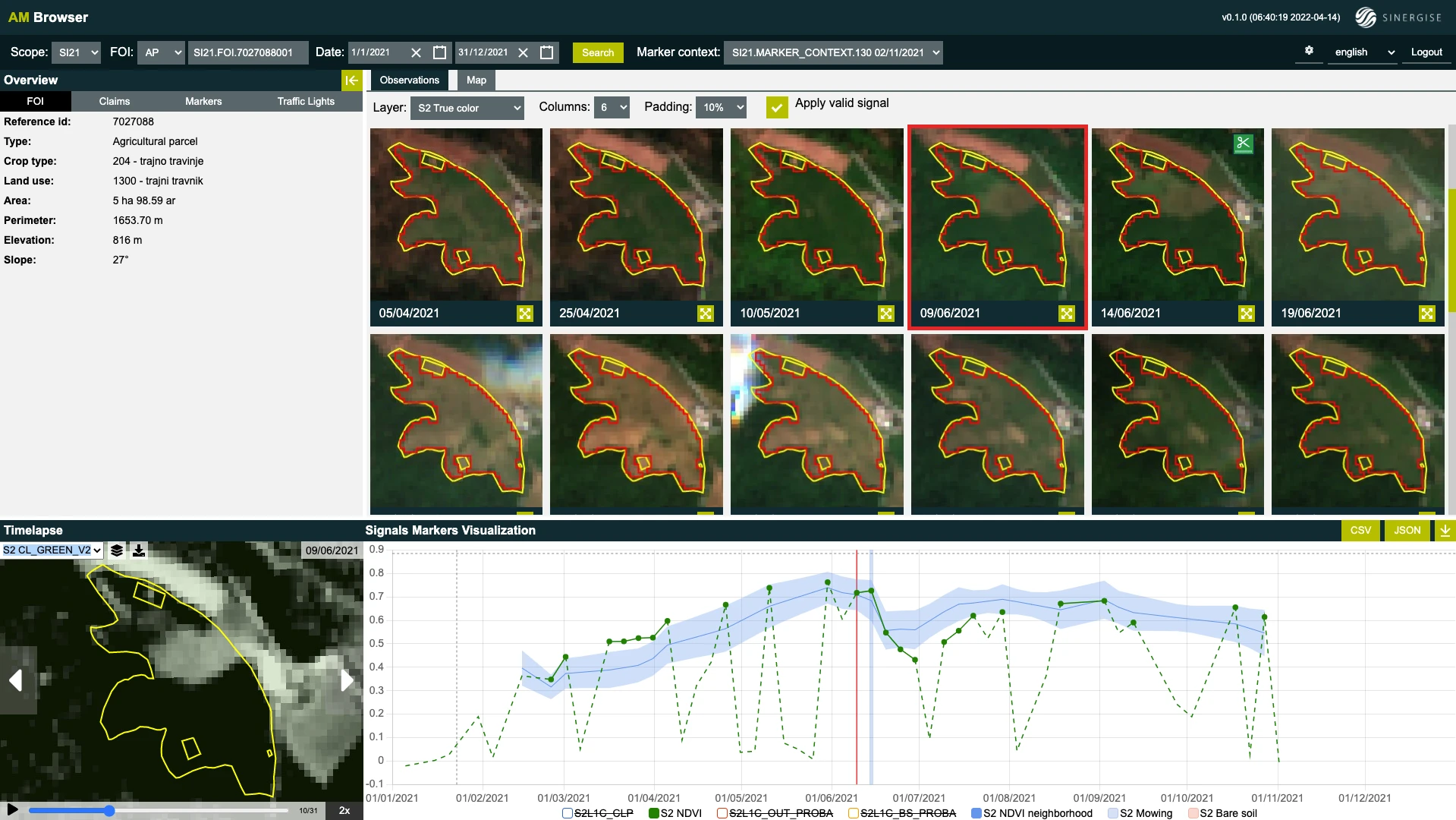
25km² [Visualize in the Browser →](https://insights.planet.com/analyze/browser/?zoom=14\&lat=-16.59673\&lng=-48.78251\&themeId=PLANET_SANDBOX\&visualizationUrl=https%3A%2F%2Fservices.sentinel-hub.com%2Fogc%2Fwms%2F11ce5d8a-4ae8-4f99-923c-334073b747a1\&datasetId=28eef896-9632-4546-a99e-cea34d74b21e\&fromTime=2022-11-17T00%3A00%3A00.000Z\&toTime=2022-11-17T23%3A59%3A59.999Z\&layerId=TRUE-COLOR\&demSource3D="MAPZEN") [![Cairo, Egypt](/data/imagery/planetscope/PS_EGY.webp)](https://insights.planet.com/analyze/browser/?zoom=14\&lat=30.05862\&lng=31.47\&themeId=PLANET_SANDBOX\&visualizationUrl=https%3A%2F%2Fservices.sentinel-hub.com%2Fogc%2Fwms%2F11ce5d8a-4ae8-4f99-923c-334073b747a1\&datasetId=28eef896-9632-4546-a99e-cea34d74b21e\&fromTime=2022-11-20T00%3A00%3A00.000Z\&toTime=2022-11-20T23%3A59%3A59.999Z\&layerId=TRUE-COLOR\&demSource3D="MAPZEN") Cairo, Egypt 2022-05-01 to 2023-04-30
25km² [Visualize in the Browser →](https://insights.planet.com/analyze/browser/?zoom=14\&lat=30.05862\&lng=31.47\&themeId=PLANET_SANDBOX\&visualizationUrl=https%3A%2F%2Fservices.sentinel-hub.com%2Fogc%2Fwms%2F11ce5d8a-4ae8-4f99-923c-334073b747a1\&datasetId=28eef896-9632-4546-a99e-cea34d74b21e\&fromTime=2022-11-20T00%3A00%3A00.000Z\&toTime=2022-11-20T23%3A59%3A59.999Z\&layerId=TRUE-COLOR\&demSource3D="MAPZEN") [![Perth, Australia](/data/imagery/planetscope/PS_AUS.webp)](https://insights.planet.com/analyze/browser/?zoom=14\&lat=-32.1112\&lng=116.0231\&themeId=PLANET_SANDBOX\&visualizationUrl=https%3A%2F%2Fservices.sentinel-hub.com%2Fogc%2Fwms%2F11ce5d8a-4ae8-4f99-923c-334073b747a1\&datasetId=28eef896-9632-4546-a99e-cea34d74b21e\&fromTime=2023-04-19T00%3A00%3A00.000Z\&toTime=2023-04-19T23%3A59%3A59.999Z\&layerId=TRUE-COLOR\&demSource3D="MAPZEN") Perth, Australia 2022-05-01 to 2023-04-30
25km² [Visualize in the Browser →](https://insights.planet.com/analyze/browser/?zoom=14\&lat=-32.1112\&lng=116.0231\&themeId=PLANET_SANDBOX\&visualizationUrl=https%3A%2F%2Fservices.sentinel-hub.com%2Fogc%2Fwms%2F11ce5d8a-4ae8-4f99-923c-334073b747a1\&datasetId=28eef896-9632-4546-a99e-cea34d74b21e\&fromTime=2023-04-19T00%3A00%3A00.000Z\&toTime=2023-04-19T23%3A59%3A59.999Z\&layerId=TRUE-COLOR\&demSource3D="MAPZEN") --- Copy for LLM[View as Markdown](https://docs.planet.com/data/imagery/planetscope/techspec/) # Technical Specification ### Download the PDF [Download PlanetScope Product Specifications →](https://assets.planet.com/docs/Planet_PSScene_Imagery_Product_Spec_letter_screen.pdf) --- Copy for LLM[View as Markdown](https://docs.planet.com/data/imagery/rapideye/) # RapidEye ![Header Thumbnail](/data/imagery/rapideye/re_thumbnail.webp) RapidEye, formerly operated by Planet, is a retired constellation of five satellites operating from 2009 to 2020. RapidEye images are approximately 5 meters per pixel resolution and are still available for download through Planet platforms. The RapidEye satellite constellation consisted of a single launch of five high-resolution satellites. ## RapidEye Imagery Products RapidEye products, such as Scene and Orthotile, are available for search and download via the Planet APIs, User Interfaces, and Integrations. The platform encodes these products as a set of Item Types and Asset Types. A **RapidEye Scene Product** is a framed scene captured by the satellite in its line scan of the Earth. Scenes within a strip overlap and are not organized according to any particular tiling grid system. RapidEye Scene Products range from 75 x 50 square kilometers to 75 x 300 square kilometers. They are represented in the Planet Platform as the `REScene` item type. A **RapidEye OrthoTile Product** is a 25 x 25 square kilometers orthorectified and tiled product generated from consecutive scenes within a strip (usually 1 or 2), based on a worldwide, fixed UTM grid system. They are represented in the Planet Platform as the `REOrthoTile` item type. ### Asset Types #### Basic Analytic Basic Analytic (`basic_analytic`) assets are non-orthorectified, calibrated, multispectral imagery products corrected for sensor artifacts and transformed to Top of Atmosphere (at-sensor) radiance. These products are designed for data science and analytic applications and for users who wish to geometrically correct the data (leveraging the associated rational polynomial coefficient Asset Type). #### Analytic Analytic (`analytic`) assets are orthorectified, calibrated, multispectral imagery products that have been corrected for sensor artifacts and terrain distortions, and transformed to Top of Atmosphere (at-sensor) radiance. These products are designed for data science and analytic applications that require imagery with accurate geolocation and cartographic projection. #### Visual Visual (`visual`) assets are orthorectified and color-corrected to optimize colors seen by the human eye, providing images as they would look if viewed from the satellite's perspective. These products are designed for simple and direct visual inspection, and can be used and ingested directly into a Geographic Information System or application. #### Surface Reflectance Surface Reflectance (`analytic_sr`) assets are orthorectified and radiometrically corrected to ensure consistency across localized atmospheric conditions and to minimize uncertainty in spectral response across time and location. These products are designed for temporal analysis and monitoring applications, especially in agriculture and forestry sectors. ### Product Naming The name of each acquired RapidEye image is designed to be unique and allow for easier recognition and sorting of the imagery. It includes the date and time of capture, the satellite's ID, product level, and product type. The name of each downloaded image product is composed of the following elements: #### RapidEye scene downloaded product name The name consists of the following elements: * `{acquisition-date}T{acquisition-time}_{satellite-id}_{product-level}_{band-product}.{extension}` ##### Example: * **2018-09-29T163919\_RE1\_1B\_band1.tif** #### RapidEye orthoTile downloaded product name The name consists of: * `{tileid}_{acquisition-date}_{satellite-id}_{product-level}_{band-product}.{extension}` ##### Example: * **1657017\_2018-09-29\_RE1\_3A\_Analytic.tif** ## Processing Steps Several processing steps are applied to RapidEye imagery to produce the data products that are available for download. ![](/assets/images/re_image_processing_chain-5f5bdd0c27d7f2f9613a905b4b480b23.webp) ### Sensor and Radiometric Calibration **Flat Field Correction:** Flat fields were collected for each optical instrument before launch. These fields were used to correct image lighting and CCD element effects to match the sensor's optimal response area. **Temporal Calibration:** To achieve cross-calibration, corrections were applied such that all RapidEye cameras read the same DN (digital number) regardless of when the image was taken during the mission lifetime. **Absolute Calibration:** As a last step, the spatially and temporally adjusted datasets were transformed from digital number values into physical based radiance values (scaled to W/(m²strμm)\*100). ### Orthorectification Removes terrain distortions. This process consists of two steps: 1. The rectification tiedown process wherein tie points are identified across the source images and a collection of reference images (ALOS, NAIP, Landsat) and RPCs are generated. 2. The actual orthorectification of the scenes using the RPCs, to remove terrain distortions. The terrain model used for the orthorectification process is derived from multiple sources (Intermap, NED, SRTM and other local elevation datasets), which are periodically updated. Snapshots of the elevation datasets used are archived (helps identify the DEM used for any given scene at any given point). ### Visual Product Processing Presents the imagery as natural color, optimized as seen by the human eye. This process consists of three steps: 1. Nominalization - Sun angle correction to account for differences in latitude and time of acquisition. This makes the imagery look like it was acquired at the same sun angle by converting the exposure time to the nominal time (noon). 2. Unsharp mask (sharpening filter) applied before the warp process. 3. Custom color curve applied post-warping. ### Surface Reflectance Product Processing Removes atmospheric effects. This process consists of the following steps: 1. Top of Atmosphere (TOA) reflectance calculation using coefficients supplied with the at-sensor radiance product. 2. Lookup table (LUT) generation using the 6SV2.1 radiative transfer code and MODIS near-real-time data inputs. 3. Conversion of TOA reflectance to surface reflectance for all combinations of selected ranges of physical conditions and for each satellite sensor type using its spectral response and estimates of the state of the atmosphere. For detailed technical information on RapidEye images, refer to [Planet Imagery Product Specification](https://planet.widen.net/content/dtzlv15tk3/original/Planet-UserDocument-CombinedImagery-ProductSpec.pdf). --- Copy for LLM[View as Markdown](https://docs.planet.com/data/imagery/rapideye/item-types/reorthotile/) # REOrthoTile ## REOrthoTile Item Type Loading resource data... Loading... ## Item Properties | Field | Description | Data Type | | ----- | ----------- | --------- | --- Copy for LLM[View as Markdown](https://docs.planet.com/data/imagery/rapideye/item-types/rescene/) # REScene ## REScene Item Type Loading resource data... Loading... ## Item Properties | Field | Description | Data Type | | ----- | ----------- | --------- | --- Copy for LLM[View as Markdown](https://docs.planet.com/data/imagery/skysat/) # SkySat ![Header Thumbnail](/data/imagery/skysat/thumbnail.webp) SkySat, operated by Planet, is a high resolution constellation of 15 satellites, able to image revisit any location on Earth up to 10x daily (a daily collection capacity of 4,000 km2/day). SkySat supports the Planet high resolution [tasking](https://docs.planet.com/platform/get-started/access-data/task-imagery.md), which allows you to choose when and where to capture SkySat imagery. SkySat produces 4-band and panchromatic imagery and is sampled at 50 centimeters per pixel when orthorectified. The SkySat satellite constellation consists of multiple launches of the Planet SkySat-C generation satellites, first launched in 2016. Each satellite is 3-axis stabilized and agile enough to slew between different targets of interest. Each satellite has four thrusters for orbital control, along with four reaction wheels and three magnetic torquers for attitude control. Currently, the SkySat constellation consists of morning and afternoon sun-synchronous satellites with an operational altitude of 475 km. The minimum and maximum latitude coverage is up to ±80°, but depends on season. SkySat collects approximately a 5.73 km swath. All SkySat satellites contain Cassegrain telescopes with a focal length of 3.6 m, with three overlapping 5.5 megapixel CMOS imaging detectors making up the focal plane. The central detector is slightly offset from the side detectors, giving SkySat imagery its unique tuning fork outline. SkySat can collect frame imagery, stereo imagery, and video in day or night collects. SkySat images are typically collected in short exposures, coregistered, and stacked to improve the SNR and GSD with super-resolution. SkySat collects RGB, NIR and panchromatic imagery. | Band | Name | Wavelength | | ---- | ------------ | ------------ | | 1 | Blue | 450 - 515 nm | | 2 | Green | 515 - 595 nm | | 3 | Red | 605 - 695 nm | | 4 | Near IR | 740 - 900 nm | | NA | Panchromatic | 450 - 900 nm | ## SkySat Imagery Products SkySat imagery products are available for search, ordering, and download via Planet's APIs, User Interfaces, and Integrations. Planet offers several `item` types for SkySat imagery. Small AOIs that are covered by a single SkySat frame image may be ordered as `SkySatScene` item. Larger strips are available as coregistered, stacked, mosaiced scenes with the `SkySatCollect` item. Videos are delivered with the `SkySatVideo` item. For `SkySatScene` and `SkySatCollect`, different levels of image processing for the final product can be specified via the `Asset` type. More information on Planet `Item` and `Asset` types is available [here](https://docs.planet.com/develop/apis/data/items.md). ### SkySat Item Types A **SkySat Scene Product** is an individual framed scene within a strip, captured by the satellite in its line-scan of the Earth. SkySat Satellites have three cameras per satellite, which capture three overlapping strips. Each of these strips contain overlapping scenes, not organized to any particular tiling grid system. SkySat Scene products are approximately 1 x 2.5 sq km in size and are represented in the Planet Platform as the `SkySatScene` item type. You can find an image that covers an area of interest larger than a SkySat Scene and order a SkySat Collect Product. A **SkySat Collect Product** is created by composing many SkySat Scenes along an imaging strip into an orthorectified segment. Collects are often composed of 60 or more scenes and will be at least 5 km long. They are represented in the Planet Platform as the `SkySatCollect` item type. This product may be easier to handle, if you're looking at larger areas of interest with SkySat imagery. Due to the image rectification process involved in creating this product, Collect is generally recommended over the Scene product when the AOI spans multiple scenes, particularly if a mosaic or composite image of the individual scenes is required. Collect performs necessary rectification steps automatically. This is especially useful for users who don't feel comfortable doing orthorectification manually. A **SkySat Video Product** is a full motion video are collected between 30 and 120 seconds by a single camera from any of the SkySat satellites. Its size is comparable to a SkySat Scene, about 1 x 2.5 square kilometers. They are represented in the Planet Platform as the `SkySatVideo` item type. ![SkySat Scene and Collect](/data/imagery/skysat/collect_and_scene.webp) SkySat Scene and Collect ### SkySat Imagery Asset Types SkySat Scene and Collect products are available for download in the form of imagery assets. Multiple asset types are available for Scene and Collect products, each with differences in radiometric processing and/or rectification. Asset Type availability varies by Item Type. Further details on the supported assets by item type are indicated on each Item Types' documentation site. **Basic L1A Panchromatic** (`basic_l1a_panchromatic_d`) assets are non-orthorectified, uncalibrated, panchromatic-only imagery products with native sensor resolution. They are typically ready two hours after capture and before all other SkySat asset types are available in the catalog. These products are designed for time-sensitive, low-latency monitoring applications. They can be geometrically corrected with associated rational polynomial coefficients (RPCs) assets derived from satellite telemetry. **Basic Analytic** (`basic_analytic`) assets are non-orthorectified, calibrated, multispectral imagery products with native sensor resolution, that have been transformed to Top of Atmosphere (at-sensor) radiance. The multispectral bands have been co-registered to each other and to the ground. Rational polynomial coefficients (RPCs) assets (ground control applied) are provided for users who wish to geometrically correct the data themselves. This product is designed for data science and analytic applications. **Basic Panchromatic** (`basic_panchromatic`) assets are non-orthorectified, calibrated, super-resolved, panchromatic-only imagery products that have been transformed to Top of Atmosphere (at-sensor) radiance. Rational Polynomial coefficients (RPCs) assets (ground control applied) are provided if you want to geometrically correct the data. A basic panchromatic image is coregistered with the associated basic analytic image. This product is designed for data science and analytic applications which depend on a wider spectral range (Pan: 450 - 900 nm). **Ortho Analytic** (`ortho_analytic`) assets are orthorectified, calibrated, multispectral imagery products with native sensor resolution that have been transformed to Top of Atmosphere (at-sensor) radiance. These products are designed for data science and analytic applications which require imagery with accurate geolocation and cartographic projection. **Ortho Analytic Surface Reflectance** (`ortho_analytic_sr`) assets are corrected for the effects of the Earth's atmosphere, accounting for the molecular composition and variation with altitude along with aerosol content. Combining the use of standard atmospheric models with the use of MODIS water vapor, ozone and aerosol data, this provides reliable and consistent surface reflectance scenes over Planet's varied constellation of satellites as part of our normal, on-demand data pipeline. **Ortho Panchromatic** (`ortho_panchromatic`) assets are orthorectified, calibrated, super-resolved, panchromatic-only imagery products that have been transformed to Top of Atmosphere (at-sensor) radiance. Final image products are sampled at 50 cm. These products are designed for data science and analytic applications which require a wider spectral range (Pan: 450 - 900 nm), highest available resolution, and accurate geolocation and cartographic projection. **Ortho Pansharpened** (`ortho_pansharpened`) assets are orthorectified, uncalibrated, super-resolved, multispectral imagery products. Lower resolution multispectral bands are sharpened to match the resolution of the super-resolved panchromatic band. Final image products are sampled at 50 cm resolution. These products are designed for multispectral applications which require highest available resolution and accurate geolocation and cartographic projection. **Ortho Visual** (`ortho_visual`) assets are orthorectified, color-corrected, super-resolved, RGB imagery products. Color corrections are applied that are optimized for the human eye, providing images as they would look if viewed from the perspective of the satellite. Lower resolution multispectral bands are sharpened by the super-resolved panchromatic band. Final image products are sampled at 50 cm resolution. These products are designed for simple and direct visual inspection, and can be used and ingested directly into a Geographic Information System or application. Additional details about formatting, calibration, and data scheme are available in the [Imagery Product Specification document](https://planet.widen.net/s/np6knvxnzh/planet-userdocument-combinedimagery-productspec). Planet customers can review our quarterly SkySat image reports [here](https://support.planet.com/hc/en-us/articles/360037649594-L1-Data-Quality-Report-for-the-SkySat-Constellation). ### SkySat Video Asset Types Download the SkySat Video for an overview of supported assets by SkySatVideo item type [here](https://docs.planet.com/data/imagery/skysat/item-types/skysatvideo.md). **Video File** (`video_file`) assets are video mp4 files, produced with Basic L1a Panchromatic scene assets captured as part of the full-motion video. Currently, no stabilization is applied to video. **Video Frames** (`video_frames`) assets are compressed folders which include all of the frames used to create the Video File, packaged as Basic L1a Panchromatic scene assets with accompanying rational polynomial coefficients (RPCs). These products are designed primarily for customers interested in using video frames for 3D reconstruction. ### Product Naming The name of each acquired SkySat image is unique and allows for easier recognition and sorting of the imagery. Currently, it includes the date and approximate time of capture, as well as the satellite id that captured it. The name of each downloaded image product is composed of the following elements: #### SkySatScene {acquisition date}\_{acquisition time}\_{satellite\_id}{camera\_id}\_{frame\_id}\_{asset}.{extension} Example: **20200814\_162132\_ssc4d3\_0021\_analytic.tif** #### SkySat Collect {acquisition date}\_{acquisition time}\_{satellite\_id}\_{frame\_id}\_{bandProduct}.{extension} Example: **20200815\_091045\_ssc6\_u0002\_visual.tif** note A `frame_id` with a leading `u`, as in `u0002` above, indicates a Collect product. A `frame_id` that is only a number, as in `0021`, indicates an individual Scene product. #### SkySat Video {acquisition date}\_{acquisition time}\_{satellite\_id}{camera\_id}\_video.mp4 Example: **20200808\_133717\_ssc3d1\_video.mp4** ## Processing Several processing steps are applied to SkySat imagery to produce the set of data products available for download. ![SkySat Processing](/data/imagery/skysat/skysat_image_processing_chain.webp) SkySat Processing ### Sensor & Radiometric Calibration **Darkfield/Offset Correction:** Corrects for sensor bias and dark noise. Master offset tables are created by averaging on-orbit darkfield collects across 5-10 degree temperature bins and applied to scenes during processing based on the CCD temperature at acquisition time. **Flat Field Correction:** Flat fields are collected for each optical instrument prior to launch. These fields are used to correct image lighting and CCD element effects to match the optimal response area of the sensor. Flat fields are routinely updated on-orbit during the satellite lifetime. **Camera Acquisition Parameter Correction:** Determines a common radiometric response for each image (regardless of exposure time, number of TDI stages, gain, camera temperature and other camera parameters). **Inter-Sensor Radiometric Response (Intra-Camera):** Cross calibrates the 3 sensors in each camera to a common relative radiometric response. The offsets between each sensor is derived using on-orbit cloud flats and the overlap regions between sensors on SkySat spacecraft. **Super Resolution (Level 1B Processing):** Super resolution is the process of creating an improved resolution image by fusing information from low resolution images, with the created higher resolution image being a better description of the scene. ### Orthorectification Removes terrain distortions. This process consists of two steps: 1. The rectification tiedown process wherein tie points are identified across the source images and a collection of reference images (ALOS, NAIP, Landsat) and RPCs are generated. 2. The actual orthorectification of the scenes using the RPCs, to remove terrain distortions. The terrain model used for the orthorectification process is derived from multiple sources (Intermap, NED, SRTM and other local elevation datasets) which are periodically updated. Snapshots of the elevation datasets used are archived (helps in identifying the DEM that was used for any given scene at any given point). ### Visual Product Processing Presents the imagery as natural color, optimized as seen by the human eye. This process consists of three steps: 1. Nominalization - Sun angle correction, to account for differences in latitude and time of acquisition. This makes the imagery appear to look like it was acquired at the same sun angle by converting the exposure time to the nominal time (noon). 2. Unsharp mask (sharpening filter) applied before the warp process. 3. Custom color curve applied post warping. ## API Access Information | API | Available | Notes | | ----------------- | --------- | --------------------------------------------------------- | | Data API | ✅ | | | Orders API | ✅ | See orders docs and bundle reference for more information | | Subscriptions API | ✅ | | | Analytics API | ❌ | | | Basemaps API | ❌ | | --- Copy for LLM[View as Markdown](https://docs.planet.com/data/imagery/skysat/item-types/skysatcollect/) # SkySatCollect ## SkySatCollect Item Type Loading resource data... Loading... ## Item Properties | Field | Description | Data Type | | ----- | ----------- | --------- | --- Copy for LLM[View as Markdown](https://docs.planet.com/data/imagery/skysat/item-types/skysatscene/) # SkySatScene ## SkySatScene Item Type Loading resource data... Loading... ## Item Properties | Field | Description | Data Type | | ----- | ----------- | --------- | --- Copy for LLM[View as Markdown](https://docs.planet.com/data/imagery/skysat/item-types/skysatvideo/) # SkySatVideo ## SkySatVideo Item Type Loading resource data... Loading... ## Item Properties | Field | Description | Data Type | | ----- | ----------- | --------- | --- Copy for LLM[View as Markdown](https://docs.planet.com/data/imagery/skysat/sandbox/) # SkySat Sandbox Data This Planet Sandbox Data collection for SkySat provides sample data over specific areas and times of interest. The data is available to paid and trial accounts that include processing units and is available under the CC-BY-NC license. Learn more about [Planet Sandbox Data](https://docs.planet.com/data/planet-sandbox-data.md). ## Data Collections Metadata | Source ID | Collection Name | Collection ID | Time Range | | -------------------------------- | ---------------------------- | ----------------------------------------- | ----------------------- | | Ortho\_analytic (analytic\_udm2) | Planet Sandbox Data - SkySat | BYOC-fc704520-fc81-439f-9016-5e162c32e736 | 2021-01-01 - 2022-12-31 | ## Planet Sandbox Data Areas This collection includes 61 sandbox regions. Download the GeoJSON file below the map for exact polygon boundaries. View all 61 regions | Location | Area (km²) | Time Range | Center (lat, lon) | | --------------------------------------------------- | ---------- | ----------------------- | ----------------- | | Madre de Dios, Province of Tambopata, Peru | 25 | 2021-08-11 – 2022-08-15 | -12.94, -70.04 | | Madre de Dios, Province of Tambopata, Peru | 25 | 2021-08-17 – 2022-08-15 | -12.93, -70.09 | | Madre de Dios, Province of Manú, Peru | 25 | 2021-08-17 – 2022-08-22 | -12.76, -70.56 | | Madre de Dios, Province of Manú, Peru | 25 | 2021-09-11 – 2021-10-28 | -12.60, -70.15 | | Acre, North Region, Brazil | 25 | 2022-10-05 – 2022-10-13 | -8.15, -70.29 | | Madre de Dios, Province of Tambopata, Peru | 33 | 2021-09-06 – 2022-08-19 | -12.98, -69.90 | | Madre de Dios, Province of Tambopata, Peru | 45 | 2021-08-11 – 2021-11-26 | -12.87, -70.01 | | Amazonas, North Region, Brazil | 25 | 2022-05-28 – 2022-07-13 | -4.73, -61.34 | | Amazonas, North Region, Brazil | 22 | 2021-05-06 – 2022-09-20 | -3.57, -69.23 | | Suriname | 81 | 2022-04-05 – 2022-08-12 | 5.10, -54.48 | | Paraná, South Region, Brazil | 23 | 2021-04-20 – 2021-05-04 | -24.36, -51.23 | | São Paulo, Southeast Region, Brazil | 25 | 2021-01-05 – 2022-12-31 | -23.61, -46.48 | | Goiás, Central-West Region, Brazil | 14 | 2022-08-05 – 2022-08-05 | -16.60, -48.80 | | Bahia, Northeast Region, Brazil | 25 | 2021-01-04 – 2022-12-28 | -9.47, -40.83 | | Paraíba, Northeast Region, Brazil | 14 | 2022-10-01 – 2022-10-04 | -7.41, -36.35 | | Cross River State, Nigeria | 25 | 2021-01-03 – 2022-11-30 | 6.66, 9.17 | | Borno State, Nigeria | 20 | 2021-10-31 – 2021-11-01 | 10.60, 11.98 | | Castile-La Mancha, Spain | 25 | 2021-02-01 – 2022-12-25 | 40.09, -4.49 | | Galicia, Spain | 25 | 2021-06-03 – 2022-09-15 | 43.10, -8.42 | | Autonomous Community of the Basque Country, Spain | 23 | 2021-06-11 – 2022-08-30 | 43.24, -3.02 | | Veneto, Italy | 25 | 2022-09-01 – 2022-10-12 | 45.90, 12.29 | | Auvergne-Rhône-Alpes, Metropolitan France, France | 25 | 2021-02-19 – 2021-09-07 | 46.33, 2.60 | | Ile-de-France, Metropolitan France, France | 19 | 2022-06-11 – 2022-06-11 | 48.31, 3.02 | | England, United Kingdom | 20 | 2022-08-12 – 2022-08-12 | 50.83, -3.81 | | Lower Saxony, Germany | 25 | 2021-04-30 – 2021-10-25 | 52.25, 9.24 | | Flevoland, Netherlands | 25 | 2021-11-18 – 2022-12-29 | 52.34, 5.52 | | England, United Kingdom | 25 | 2021-04-07 – 2022-06-26 | 53.76, -1.33 | | Central District, Botswana | 14 | 2022-12-05 – 2022-12-27 | -21.65, 24.49 | | Oshikoto, Namibia | 25 | 2021-05-18 – 2022-10-26 | -19.02, 16.74 | | Malanje Province, Angola | 21 | 2021-09-13 – 2022-02-11 | -9.56, 16.33 | | Western Bahr el Ghazal State, South Sudan | 25 | 2021-01-03 – 2022-12-01 | 7.71, 27.98 | | Borno State, Nigeria | 24 | 2021-03-05 – 2022-05-02 | 11.78, 13.17 | | Borno State, Nigeria | 25 | 2021-02-05 – 2022-04-14 | 12.67, 13.60 | | Bulgaria | 25 | 2021-06-04 – 2021-07-11 | 42.39, 25.96 | | Bulgaria | 23 | 2021-08-10 – 2022-05-23 | 43.79, 23.30 | | Southwest, Czechia | 24 | 2021-06-25 – 2021-06-25 | 49.29, 14.50 | | Czechia | 13 | 2022-12-16 – 2022-12-16 | 49.74, 15.48 | | Brandenburg, Germany | 25 | 2021-02-12 – 2022-02-21 | 52.94, 12.64 | | KwaZulu-Natal, South Africa | 19 | 2021-03-05 – 2022-12-14 | -28.94, 31.54 | | Tigray, Ethiopia | 44 | 2021-03-31 – 2022-08-29 | 14.07, 36.57 | | Cairo, Egypt | 25 | 2021-04-16 – 2022-09-22 | 30.06, 31.47 | | Gaza Strip, Palestinian Territories | 25 | 2021-05-20 – 2022-12-18 | 31.28, 34.27 | | Kursk Oblast, Central Federal District, Russia | 20 | 2022-04-10 – 2022-04-15 | 51.98, 35.60 | | Tver Oblast, Central Federal District, Russia | 21 | 2021-02-08 – 2022-03-22 | 56.38, 34.11 | | Galgaduud, Somalia | 24 | 2021-01-03 – 2022-12-01 | 6.15, 46.63 | | Baghdad Governorate, Iraq | 25 | 2021-01-26 – 2022-10-04 | 33.32, 44.45 | | West Azerbaijan Province, Iran | 23 | 2021-11-09 – 2022-05-01 | 36.15, 45.48 | | Eastern Anatolia Region, Turkey | 25 | 2022-06-24 – 2022-12-21 | 38.34, 38.15 | | Karabakh, Azerbaijan | 25 | 2021-02-12 – 2022-11-13 | 39.82, 46.75 | | Karabakh, Azerbaijan | 25 | 2022-08-20 – 2022-08-20 | 40.03, 46.69 | | Astrakhan Oblast, Southern Federal District, Russia | 25 | 2021-02-18 – 2022-03-24 | 47.76, 46.40 | | Western Australia, Australia | 25 | 2021-02-14 – 2022-10-05 | -32.34, 115.80 | | Western Australia, Australia | 25 | 2021-01-01 – 2022-12-28 | -32.11, 116.01 | | Stung Treng, Cambodia | 20 | 2021-03-06 – 2021-08-06 | 13.18, 105.85 | | Maharashtra, India | 25 | 2022-09-03 – 2022-09-03 | 17.21, 73.64 | | Chattogram Division, Bangladesh | 25 | 2021-03-23 – 2022-09-23 | 21.19, 92.18 | | Jharkhand, India | 25 | 2021-01-13 – 2022-11-07 | 22.78, 86.07 | | Sikkim, India | 25 | 2022-08-12 – 2022-08-15 | 27.30, 88.32 | | Surxondaryo Region, Uzbekistan | 16 | 2021-09-05 – 2021-09-05 | 37.37, 66.73 | | North Pyongan, North Korea | 25 | 2021-03-22 – 2022-06-15 | 39.99, 124.61 | | Japan | 15 | 2021-09-07 – 2021-09-07 | 40.16, 140.92 | [Download GeoJSON](https://docs.planet.com/data/imagery/skysat/polygons.geojson) ## Highlights [![Bahia, Brazil](/data/imagery/skysat/skysat.webp)](https://insights.planet.com/analyze/browser/?zoom=14\&lat=-9.46769\&lng=-40.83146\&themeId=PLANET_SANDBOX\&visualizationUrl=https%3A%2F%2Fservices.sentinel-hub.com%2Fogc%2Fwms%2Fc0d9df19-9fb2-4191-89bd-4168678def5d\&datasetId=fc704520-fc81-439f-9016-5e162c32e736\&fromTime=2022-05-07T00%3A00%3A00.000Z\&toTime=2022-05-07T23%3A59%3A59.999Z\&layerId=TRUE-COLOR\&demSource3D="MAPZEN") Bahia, Brazil 2021-01-04 to 2022-12-28
25km² [Visualize in the Browser →](https://insights.planet.com/analyze/browser/?zoom=14\&lat=-9.46769\&lng=-40.83146\&themeId=PLANET_SANDBOX\&visualizationUrl=https%3A%2F%2Fservices.sentinel-hub.com%2Fogc%2Fwms%2Fc0d9df19-9fb2-4191-89bd-4168678def5d\&datasetId=fc704520-fc81-439f-9016-5e162c32e736\&fromTime=2022-05-07T00%3A00%3A00.000Z\&toTime=2022-05-07T23%3A59%3A59.999Z\&layerId=TRUE-COLOR\&demSource3D="MAPZEN") [![Cairo, Egypt](/data/imagery/skysat/SS_EGY.webp)](https://insights.planet.com/analyze/browser/?zoom=14\&lat=30.05862\&lng=31.47\&themeId=PLANET_SANDBOX\&visualizationUrl=https%3A%2F%2Fservices.sentinel-hub.com%2Fogc%2Fwms%2Fc0d9df19-9fb2-4191-89bd-4168678def5d\&datasetId=fc704520-fc81-439f-9016-5e162c32e736\&fromTime=2022-08-19T00%3A00%3A00.000Z\&toTime=2022-08-19T23%3A59%3A59.999Z\&layerId=TRUE-COLOR\&demSource3D="MAPZEN") Cairo, Egypt 2021-04-16 to 2022-09-22
25km² [Visualize in the Browser →](https://insights.planet.com/analyze/browser/?zoom=14\&lat=30.05862\&lng=31.47\&themeId=PLANET_SANDBOX\&visualizationUrl=https%3A%2F%2Fservices.sentinel-hub.com%2Fogc%2Fwms%2Fc0d9df19-9fb2-4191-89bd-4168678def5d\&datasetId=fc704520-fc81-439f-9016-5e162c32e736\&fromTime=2022-08-19T00%3A00%3A00.000Z\&toTime=2022-08-19T23%3A59%3A59.999Z\&layerId=TRUE-COLOR\&demSource3D="MAPZEN") [![Perth, Australia](/data/imagery/skysat/SS_AUS.webp)](https://insights.planet.com/analyze/browser/?zoom=14\&lat=-32.1112\&lng=116.0231\&themeId=PLANET_SANDBOX\&visualizationUrl=https%3A%2F%2Fservices.sentinel-hub.com%2Fogc%2Fwms%2Fc0d9df19-9fb2-4191-89bd-4168678def5d\&datasetId=fc704520-fc81-439f-9016-5e162c32e736\&fromTime=2022-10-19T00%3A00%3A00.000Z\&toTime=2022-10-19T23%3A59%3A59.999Z\&layerId=TRUE-COLOR\&demSource3D="MAPZEN") Perth, Australia 2021-01-01 to 2022-12-28
25km² [Visualize in the Browser →](https://insights.planet.com/analyze/browser/?zoom=14\&lat=-32.1112\&lng=116.0231\&themeId=PLANET_SANDBOX\&visualizationUrl=https%3A%2F%2Fservices.sentinel-hub.com%2Fogc%2Fwms%2Fc0d9df19-9fb2-4191-89bd-4168678def5d\&datasetId=fc704520-fc81-439f-9016-5e162c32e736\&fromTime=2022-10-19T00%3A00%3A00.000Z\&toTime=2022-10-19T23%3A59%3A59.999Z\&layerId=TRUE-COLOR\&demSource3D="MAPZEN") --- Copy for LLM[View as Markdown](https://docs.planet.com/data/imagery/skysat/techspec/) # Technical Specification ### Download the PDF [Download Planet Imagery Product Specifications →](https://assets.planet.com/docs/Planet_Combined_Imagery_Product_Specs_letter_screen.pdf) --- Copy for LLM[View as Markdown](https://docs.planet.com/data/imagery/superres/) ![Header Thumbnail](/data/imagery/superres/central-park-manhattan-new-york-super-res.webp) # SuperRes Overview Planet SuperRes uses the Enhanced Super-Resolution Generative Adversarial Network (ESRGAN) with a collection of 120,000 pairs of SkySat and PlanetScope imagery with a perceptual loss training technique to produce imagery that looks natural and remains faithful to the ground truth. We include a confidence layer to help assess the degree of accuracy of the generated pixel by evaluating various sources of error. Planet SuperRes is currently available as SuperRes [Mosaics](https://docs.planet.com/data/imagery/mosaics.md#superres-mosaics) and SuperRes [PlanetScope Scenes](https://docs.planet.com/data/imagery/planetscope/psscene.md). To learn more about Planet SuperRes, visit [Planet University - Introduction to Planet SuperRes](https://university.planet.com/introduction-to-planet-superres). They share the model features described below: ![Vinkeveen-Utrecht, Netherlands SuperRes Visual Mosaic November 2025](/data/imagery/superres/Vinkeveen-Utrecht_Netherlands_super_res.webp) Vinkeveen-Utrecht, Netherlands SuperRes Visual Mosaic November 2025 | | | | ---------------------- | ----------------------------------------------------------------------------------------------------------------------------------------------------------------------------------------------------------------------------------------------------------------------------------------------- | | Product Specifications | - - 2 meter resolution prediction: AI-enhanced resolution (reprojected to 2.4 m at the equator).- - Confidence layer: A per-pixel map identifying areas where the AI has high certainty versus where it made inferences.* * Self-service access: Direct access through familiar APIs and tools. | ## The Training Dataset The training dataset is the foundation of Planet Visual SuperRes. It consists of 120,476 high-quality image pairs, each comprising a 3 m PlanetScope scene and a 0.5 m SkySat scene of the same location. Dataset quality is ensured through strict curation standards: * **Temporal consistency:** Every pair was captured within a 12-hour window to minimize change on the ground between acquisitions. * **Geometric precision:** Sub-pixel co-registration was achieved via phase correlation; pairs with a phase correlation error exceeding 0.2 were discarded. * **Radiometric normalization:** Per-pixel normalization aligns the SkySat spectral response to PlanetScope, preventing radiometric artifacts in the model output. * **Clarity:** A minimum 95% clear-sky requirement was applied to both images in every pair, eliminating cloud contamination. The dataset spans diverse geographies, seasons, and land cover types — providing the broad training signal needed for reliable performance at a global scale. It is split into 100,476 training pairs, 10,000 validation pairs, and a held-out test set of 10,000 pairs. ## Model Architecture and Training Planet Visual SuperRes uses an Enhanced Super-Resolution Generative Adversarial Network (ESRGAN), a leading generative AI approach for single-image super-resolution. ![SuperRes Visual Mosaic, October 2025](/data/imagery/superres/superres-visual-mosaic-oct-2025-1.webp) SuperRes Visual Mosaic, October 2025 Key architectural elements include: * Residual-in-Residual Dense Blocks (RRDBs): Replace traditional residual blocks with denser connections for improved feature representation and training stability. * Perceptual Loss Function: Combines pixel-wise loss with perceptual loss derived from a pre-trained deep network, training the model to produce outputs that look sharp and natural to the human eye — not just pixel-accurate. * Adversarial Training: A discriminator network enforces realistic textures and fine details, enabling sharper outputs than traditional bicubic or convolutional methods. The production 1.5x model was further optimized for deployment: input channels were reduced from 8 to 4 bands with no performance loss, iterative pruning reduced the computational footprint, and the final model was quantized to half-precision (float16) for efficient inference at scale. ## The Confidence Layer The Confidence Layer is an auxiliary output channel added to the ESRGAN generator network. It is trained concurrently with the primary super-resolution task to predict the expected Mean Absolute Error (MAE) between the model's output and ground truth image, using an L1 loss function. At inference time, the layer produces a per-pixel MAE estimate from the low-resolution input alone with no reference high-resolution image required. The raw MAE output is rescaled to a 0–100 confidence score: * Confidence = 100 \* 1 - min((MAE / 2500), 1) ![SuperRes Visual Mosaic, October 2025](/data/imagery/superres/superres-visual-mosaic-oct-2025-2.webp) SuperRes Visual Mosaic, October 2025 ## Reliable Performance The production 1.5x model was evaluated against the 10,000-image held-out test set. Our primary metric is Learned Perceptual Image Patch Similarity (LPIPS), which evaluates image similarity based on deep network feature maps (AlexNet) and aligns most closely with human visual perception. We report 1 − LPIPS so that higher scores indicate better perceptual quality. | Metric | Score | | ----------------------------------------------------- | ----- | | 1 − Learned Perceptual Image Patch Similarity (LPIPS) | 0.961 | | Peak Signal-to-Noise Ratio (PSNR) | 33.53 | | Structural Similarity Index Measure (SSIM) | 0.876 | | Confidence Layer Accuracy\* | 0.993 | \**Confidence Layer Accuracy provides a direct comparison between the ground truth MAE and our predicted MAE.* In a world where the gap between coverage and clarity has constrained what satellite imagery can deliver, Planet Visual SuperRes offers something new: the persistent, near-daily global reach of PlanetScope, with sharper imagery that makes features easier to see, characterize, and monitor at scale. With a purpose-built training dataset, a model tuned for human visual perception, and a built-in Confidence Layer that provides per-pixel transparency, Planet SuperRes gives analysts a clearer view of the world — and more time to focus on what they see in it. ## Disclaimer Neural networks, including the processes used to create SuperRes Mosaics are a form of artificial intelligence (AI). While the per-pixel confidence layer (noted above) is intended to help Licensee identify the accuracy of each pixel of SuperRes, the SuperRes neural network may generate incorrect, incomplete, or misleading information, and may fail to identify (or may hallucinate) features or objects depicted. Planet does not warrant or guarantee the accuracy, completeness, or suitability of SuperRes Mosaics. Licensee is solely responsible for reviewing, validating, and approving any SuperRes pixel, particularly before Licensee takes action based on such SuperRes pixel, including, without limitation, visual comparison of each pixel with the corresponding standard visual mosaic. --- Copy for LLM[View as Markdown](https://docs.planet.com/data/imagery/tanager/) # Tanager ![Header Thumbnail](/data/imagery/tanager/tanager-plume.webp) ### Constellation & Sensor Overview The Tanager satellite is an imaging spectrometer capturing approximately 426 Bands with \~5 nm spacing between an approximate range of 380-2500 nm at 30 meters per pixel resolution, with the first launched in August 2024. Planet intends to launch additional Tanager satellites to meet market demands over the coming years. Each satellite is 3-axis stabilized and agile enough to slew between different targets of interest. Each satellite has a single electric propulsion (EP) thruster for orbital control, along with four reaction wheels and three magnetic torquers for attitude control. All Tanagers contain three-mirror anastigmat (TMA) telescopes with a focal length of 400 mm and Dyson form spectrometers, with a 640x480 pixel Mercury-Cadmium-Telluride (MCT) detector as the focal plane array. #### Sensitivity Collection Modes Tanager's hyperspectral imaging employs a minimum integration time of 8 ms, resulting in an approximately 58 m along-track pixel length in pushbroom mode, which causes pixels in geometrically corrected images to be rectangular, and for most use cases this pixel stretching is generally an undesirable effect. To mitigate this elongation and enhance signal-to-noise ratio (SNR), Tanager utilizes a technique called 'back-nodding.' This maneuver allows imaging to begin before and continue after the satellite passes directly over the target area, extending capture time and improving SNR for smaller regions. Find the table summary below describing each mode's minimum to maximum length. | TANAGER SENSITIVITY MODE DIMENSIONS | | | | ----------------------------------- | ----------------------------------------- | ----- | | Mode | Minimum to Maximum Collection Length (km) | Width | | Maximum Sensitivity (4x8ms) | 18 to 65.9 km | 18 km | | High Sensitivity (3x8ms) | 18 to 91.5 km | 18 km | | Medium Sensitivity (2x8ms) | 18 to 153.1 km | 18 km | | Standard Sensitivity (1x8ms) | 18 to 481.2 km | 18 km | | Glint (1x8) | 18 to 481.2 km | 18 km | ##### Standard Sensitivity Collection Mode In the Standard Sensitivity collection mode, also referred to as 1x8 ms, Tanager will perform back nodding to slow down its ground scan rate just enough to avoid pixel stretching. The goal of this mode is to maximize the swath length while still maintaining square pixels. ##### Maximum Sensitivity Collection Mode In the Maximum Sensitivity collection mode, also referred to as 4x8 ms, Tanager will perform much faster back nodding to drastically slow down its ground scan rate to achieve the highest possible SNR, allowing each point to be “seen” for a \~4 times longer duration. Because of this, the effective frame rate that is achieved is equivalent to 32 ms of exposure. The goal of this variant is to optimize SNR while remaining within the envelope of Tanager’s agility and orbital geometry. ### Tanager Imagery Products #### Tanager Chunking Strategy A single Tanager collection can be quite long and in order to process and deliver Tanager assets with more reasonable file sizes, the collections will be dynamically chunked. Each collect will be separated into TanagerScenes based on a set of rules: 1. A scene is at least 325 lines long. 2. A scene is at most 750 lines long. 3. The strategy seeks to produce square-ish scenes. 4. All scenes within a single collection are approximately the same size. The worst case scenario is that a collect will have only two different scene sizes. These two sizes will vary by only a single line. Example chunking below. Each | BOX | is a TanagerScene. 1700 line collect: | 0:567 | 567:1134 | 1134:1700 | 2600 line collect: | 0:650 | 650:1300 | 1300:1950 | 1950:2600 | #### Imagery Item Type Tanager Imagery products are available as either individual Basic or Ortho Scenes and Radiance or Surface Reflectance. Tanager imagery utilizes a native file format of HDF5. These products can be obtained from the Planet APIs through the TanagerScene item type. A **Tanager Scene Product** is an individual framed scene within a strip, captured by the satellite in its line-scan of the Earth. Tanager Scene products have a swath width of 18km and the length is variable in size dependent on Planet chunking. They are represented in the Planet Platform as the `TanagerScene` item type. #### Imagery Asset Types Tanager Scene products are available for download in the form of imagery assets. Multiple asset types are made available for Scene and Collect products, each with differences in radiometric processing and/or rectification. Asset Type availability varies by Item Type. You can find an overview of supported assets by item type here: [TanagerScene Supported Assets-Types](https://docs.planet.com/data/imagery/tanager/item-types/tanagerscene.md) You can find our complete [Imagery Product Specification here](https://planet.widen.net/s/wq9dsgzvv6/planet-userdocumentation-tanager). ### Tanager Methane Products #### Methane Item Type Each TanagerMethane item has had an automated methane detection algorithm run on it, derived from a matched filter (doi:10.5194/amt-8-4383-2015). TanagerMethane products are only offered in their orthorectified format. These products can be obtained from the Planet APIs through the TanagerScene item type. A **Tanager Methane Product** is representative of a methane detection attempt on a TanagerScene item. They have the same extent as a TanagerScene. They are represented in the Planet Platform as the `TanagerMethane` item type. #### Methane Asset Types Tanager Methane products are available for download in the form of imagery and geographic feature assets. Multiple asset types are made available for Methane products, each with differences in publication latency. Asset Type availability varies by Item Type. You can find an overview of supported assets by item type here: [TanagerMethane Supported Assets-Types](https://docs.planet.com/data/imagery/tanager/item-types/tanagermethane.md) ### Product Naming The name of each Tanager image and methane product is designed to be unique and allow for easier recognition and sorting. The name of each downloaded image product is composed of the following elements: *TanagerScene* `{acquisition-date}_{acquisition-time}_{acquisition-time-seconds-hundredths}_{satellite-id}_{asset-type}.{ext}` * Example: `20241005_062757_84_4001_ortho_radiance_hdf5.h5` * Searchable product in Data API is: TanagerScene `20241005_062757_84_4001` *TanagerMethane* TanagerMethane uses the same naming convention as TanagerScene. All TanagerMethane items have a corresponding TanagerScene item. However, TanagerMethane is only created where methane detection was requested, so many TanagerScene items will not have a corresponding TanagerMethane item. `{acquisition-date}_{acquisition-time}_{acquisition-time-seconds-hundredths}_{satellite-id}_{asset-type}.{ext}` * Example: `20241005_062752_00_4001_ortho_ql_ch4.tif` * Searchable product in Data API is: TanagerMethane `20241005_062752_00_4001` ### Processing Several processing steps are applied to Tanager imagery to produce the set of data products available for download. | TANAGER PROCESSING STEPS | | | ------------------------------------------ | ------------------------------------------------------------------------------------------------------------------------------------------------------------------------------------------------------------------------------------------------------------------------------------------------------------------------------------------------------------------------------------------------------------------------------------------------------------------------------------------------------------------------------------------------------------------------------------------------------------------------------------------------------------------------------------------------------------------------------------------------------------------------------------------------------------------------------------ | | Step | Description | | Dark Subtraction | Corrects for sensor bias and dark level to ensure that zero illumination corresponds to zero radiance. The correction is updated frequently by averaging dark frames acquired over the non-sunlit side of Earth. | | Pedestal Correction | Subtracts remaining residual error in the zero point after the dark frame is subtracted so that the numerical zero is equivalent to the radiometric zero. This residual is estimated by computing the median value of masked pixels located at the edges of the detector, which are physically blocked from external illumination. | | Flat Field Correction | Corrects relative differences in pixel sensitivities to match those in the optimal response area of the sensor. Flat fields are collected for each optical instrument in lab conditions prior to launch, and are routinely updated on-orbit during the satellite lifetime. | | Bad Pixel Correction | Fills in defective pixels on the detector following the method described in Chapman et al. (2019), which replaces pixels by linearly interpolating to the most similar spectrum within the frame. | | Optical Scatter Correction | Removes stray light artifacts from scatter in the optical elements to bring the spectral response function (SRF) towards a Gaussian distribution. These artifacts are modeled as concentric Gaussians convolved with the original spectrum, so correction involves deconvolving the stray response components from the spectrum with a method outlined in Thompson et al. (2018a). | | Optical Ghost Correction | Follows the correction approach of Zandbergen et al. (2020) to remove structured stray light artifacts (“ghosts”) that arise due to unwanted reflections within the optics. A ghost image is predicted for each frame and subsequently subtracted to remove the stray signal. | | Absolute Radiometric Calibration | Converts the observations from Digital Number (DN) values into physical radiance units (W/(m²*sr*μm)). | | Order Sorting Filter (OSF) Seam Correction | Interpolates over the radiometrically suspect rows where the order sorting filter (OSF) seams are located. | | Visual Product Processing | Presents the imagery as natural color, as seen by the human eye. Only applied to the ortho\_visual asset type. | | Orthorectification | The orthorectification process is a method to correct the geographic location of imagery. The orthorectification process depends on the accuracy of the reference imagery, the terrain model, satellite and sensor parameters. OneAtlas Airbus imagery is used as reference images during Tanager orthorectification and the terrain model used for the orthorectification process is derived from multiple sources (SRTM, Intermap, and other local elevation datasets) which are periodically updated. The orthorectification process consists of two key steps. The first step is a feature-based approach for coarse model refinement followed by area-based matching for fine model refinement. The algorithm provides an improved sensor model of the satellite state and sensor, allowing for more accurate georectification. | | Atmospheric Correction | Removes atmospheric effects and estimates surface reflectance. Per pixel surface reflectance values are calculated using the ISOFIT (v2.9.5) (Imaging Spectrometer Optimal FITting) python package. This uses an optimal estimation method for simultaneously solving for both the atmospheric composition and surface reflectance values using hyperspectral radiance imagery as the input. | --- Copy for LLM[View as Markdown](https://docs.planet.com/data/imagery/tanager/item-types/tanagermethane/) # TanagerMethane ## Methane Products Overview Each TanagerMethane item has an automated methane detection algorithm run on it, derived from a matched filter (doi:10.5194/amt-8-4383-2015). TanagerMethane products are only offered in their orthorectified format. These products can be obtained from the Planet APIs using the TanagerMethane item type. A **Tanager Methane Product** is representative of a methane detection attempt on a TanagerScene item. They have the same extent as a TanagerScene. They are represented in the Planet Platform as the `TanagerMethane` item type. The Methane QuickLook (MQL) bundle is designed for easy interpretation by methane experts with limited remote sensing knowledge. Within each bundle, you can access multiple imagery assets listed below for their purposes. ### Tanager Methane QuickLook Products Tanager’s Methane QuickLook is a low-latency, derived methane product that reveals point source emission locations and estimates of magnitude in kg/hr for observed plumes. It will be delivered to customers within 72 hours of acquisition, enabling you to identify and take action quickly when emissions are detected. ## Methane Plume Metadata Relevant for `ql_ch4_json` TanagerMethane assets. | Parameter | Description | Type | | ------------------------ | ------------------------------------------------------------------------------------------------------------------------------------------------------------------------------------------------------------------------------------------------------------------- | -------- | | plume\_id | Unique identifier for each plume. The format is `_`. The “part” postfix (For example, A, B, C) identifies multiple plumes captured in the same image in the order they were detected. | string | | plume\_quality | \*\* This field is used for Methane QuickLook, ql\_ch4\_json asset-type. \*\* Qualitative assessment of plume quality captured by a human operator during the plume detection process (good, questionable, or bad). More on the Plume quality classification below. | string | | plume\_provider | Identifies the organization who identified the plume. | string | | plume\_provider\_id | Plume ID according to the `plume_provider`. Planet assigns a new plume ID to match existing naming conventions. | string | | plume\_provider\_version | Plume provenance information. This information is not directly useful to customers, but can be used by Planet and the `plume_provider` to inspect data quality issues. | string | | datetime | Date and time of the acquisition in Coordinated Universal Time (UTC). | datetime | | ime | The total kilograms (kg) of methane in a plume above the background concentration at the time of image capture. | float | | fetch | Plume length, meters (m) | float | | emission | Quantified emission rate of a plume, estimated using the Integrated Methane Enhancement method. (Duren et al., 2019 - "California's Methane Super-Emitters", Nature) | | | emission\_uncertainty | The uncertainty in an emission rate is derived from uncertainty in IME and wind speed. | | | wind\_speed\_avg | Mean wind speed m/s | float | | wind\_speed\_std | Standard deviation wind speed m/s | float | | wind\_direction\_avg | Wind direction (degrees) | float | | wind\_direction\_std | Wind direction standard deviation (degrees) | float | | wind\_source | Wind source from reanalysis. (For example, Openmeteo, HRRR, ERA5) | string | | strip\_id | Strip ID of the Tanager collect used for plume detection. | string | ### Plume Quality Classification Planet classifies detected plumes into three categories: `Good`, `Questionable`, and `Bad`, based on the following criteria: * `Good`: The plume is unambiguous, with a well-defined shape and minimal artifacts, making it reliable for further analysis. * `Questionable`: The plume is clearly present, but there are issues. For example: irregular shape or retrieval artifacts that could affect the accuracy of quantification. A post-emission QC process will also assess whether `Questionable` plumes are suitable for publishing an emission rate or if only the detection will be reported. * `Bad`: It is unclear whether the detected feature is a plume. However, this is not a final state. After an initial review, a secondary post-emission quality control process is conducted. This review determines whether the detection should be discarded or reclassified as `Questionable`. ## TanagerMethane Item Type Loading resource data... Loading... ## Item Properties | Field | Description | Data Type | | ----- | ----------- | --------- | --- Copy for LLM[View as Markdown](https://docs.planet.com/data/imagery/tanager/item-types/tanagerscene/) # TanagerScene ## Imagery Products Overview The TanagerScene products include Visual, Radiance, and Surface Reflectance hyperspectral imagery in HDF5 file format. ### Tanager Chunking Strategy A single Tanager collection can be long and to process and deliver Tanager assets with more reasonable file sizes, the collections are dynamically chunked. Each collect is separated into TanagerScenes based on the following set of rules: 1. A scene is at least 325 lines long. 2. A scene is at most 750 lines long. 3. The strategy seeks to produce square-ish scenes. 4. All scenes within a single collection are approximately the same size. The worst case scenario is that a collect will have only two different scene sizes. These two sizes will vary by only a single line. Example chunking below. Each | BOX | is a TanagerScene. 1700 line collect: | 0:567 | 567:1134 | 1134:1700 | 2600 line collect: | 0:650 | 650:1300 | 1300:1950 | 1950:2600 | ### Tanager Ortho Products The Tanager Ortho Scene product is orthorectified and the product was designed for a wide variety of applications that require imagery with an accurate geolocation and cartographic projection. It has been processed to remove distortions caused by terrain and can be used for cartographic purposes. The Ortho Scenes are delivered as visual (RGB), top-of-atmosphere radiance and surface reflectance products. Ortho Scenes are radiometrically-, sensor-, and geometrically-corrected products that are projected to a cartographic map projection. The geometric correction uses fine Digital Elevation Models (DEMs) with a post spacing of between 10 and 90 meters. Ground Control Points (GCPs) are used in the creation of every image and the accuracy of the product will vary from region to region based on available GCPs. Computer vision algorithms are used for extracting feature points such as OpenCV’s STAR keypoint detector and FREAK keypoint extractor. The GCP and tiepoint matching is done using a combination of RANSAC, phase correlation and mutual information. ### Tanager Basic Products The Tanager Basic Scene products are unorthorectified, providing imagery as seen from Tanager without any geolocation corrections inherent in the imaging process. It has a scene based framing, and is not mapped to a cartographic projection. This product line is available in HDF-EOS5 format. The Tanager Basic Scene product contains the hyperspectral data in image space and a separate geolocation array (longitude and latitude information) that has been processed to remove distortions caused by terrain and geometric sensor distortions. The Basic Scene product is designed for users that want to orthorectify the product themselves with the help of the provided geolocation array or for users with advanced image processing capabilities and a desire to geometrically correct the product themselves. ## TanagerScene Item Type Loading resource data... Loading... ## Item Properties | Field | Description | Data Type | | ----- | ----------- | --------- | --- Copy for LLM[View as Markdown](https://docs.planet.com/data/imagery/tanager/techspec/) # Technical Specification ### Download the PDF [Download Tanager Product Specifications →](https://planet.widen.net/s/g7hkc69nvr/planet-userdocumentation-tanager) --- Copy for LLM[View as Markdown](https://docs.planet.com/data/imagery/udm/) # Usable Data Mask ![Header Thumbnail](/data/imagery/udm/clouds_shropshire_england_20231103_101837_21_2455_toar_with_cloud_map_6m_CLOUDS_flat_rotated_2880px_geo.webp) ## Overview Clouds, aerosols, and other surface conditions can impact the radiometry and usability of Earth observation data. To improve the consistency of data analysis of satellite imagery for research or commercial applications, Planet provides the Usable Data Mask (UDM) to accurately classify these phenomena in every image published in the Planet data catalog. UDM classifies each pixel in an image as Clear, Cloud, Haze, Cloud Shadow or Snow, allowing users to determine which pixels are usable for their analysis. UDM2.1 is the latest version developed by Planet, provided in multiband GeoTIFF format, with each band corresponding to a different semantic class and two additional bands offering supplementary information. ## Archive Availability As of November 29, 2023 all PlanetScope and SkySat imagery will be processed by UDM2.1. Any imagery acquired prior to November 29, 2023 were processed by UDM2.0. **Planetscope:** Usable Data Masks are available globally for PlanetScope imagery beginning in August, 2018. In specific agricultural regions, UDMs are available from January 2018. A small percentage of PlanetScope imagery after August 2018 will not include the UDM2 asset due to rectification or image processing failures. **SkySat:** Usable Data Masks are available for the SkySat imagery beginning from 2017. In rare instances, a UDM2 asset may not be available for specific SkySat items. **Pelican:** All Usable Data Masks for Pelican imagery will be processed by UDM2.1. ## Key differences between UDM2.1 and UDM2.0 Planet published a new Usable Data Mask version (UDM2.1) in November, 2023. UDM2.1 has significantly improved classification accuracy compared to previous versions of the product. In addition, there are some key differences between the UDM versions: * The classification schema for UDM was modified for UDM2.1 to contain a single Haze class, producing a more consistent, accurate, and understood product. * The Heavy Haze class from UDM2.0 has been deprecated in UDM2.1. This class had lower predictive accuracy, and was commonly misclassified with the Cloud and Light Haze classes. * A new dataset of ground truth images was labelled to train new models with the updated classification schema. See [Methodology](#udm21-classification-methodology) for more detail. * The Cloud class is defined as regions of a scene containing opaque atmospheric interference; objects on the ground cannot be seen through Cloud. Alternatively, Haze is defined as any interference that *can* be seen through to the ground. * In some instances, the Near-Infrared (NIR) band is required to distinguish between Cloud and Haze, due to the "atmospheric window" of infrared wavelengths. As a result, Haze classifications in UDM will occasionally appear opaque in a Visual product, but are transparent when viewed as a false color image with the NIR band. note The formatting has not changed between UDM2.0 to UDM2.1; the product still contains 8-bands for backwards compatibility. The prior Light Haze band (band 4) now contains the UDM2.1 Haze classification values. The values for the Heavy Haze band (band 5) and the heavy\_haze\_percent metadata will always be 0 for UDM2.1. ## UDM2.1 product bands The UDM2.1 asset is delivered as a 8-band GeoTIFF file, with the following bands and values: | Band | Class | Pixel Value Range | Description | | ---- | --------------- | ----------------- | ------------------------------------------------------------------------------------------------------------------------------------------------------------------------------------------------------------------------------------------------------------------------------------------------------------------------------------------------------------------------------------------------------------------------------------------------------------------------------------------------------------------------------------------------- | | 1 | Clear | 0,1 | Regions of a scene that are free of cloud, haze, cloud shadow and/or snow. | | 2 | Snow | 0,1 | Regions of a scene that are covered with snow or ice. | | 3 | Cloud Shadow | 0,1 | Shadows caused by clouds or haze and not by mountains, buildings, or other terrain features. | | 4 | Light Haze | 0,1 | Regions of a scene with thin, filamentous clouds, soot, dust, and smoke. You can see ground objects through haze. | | 5 | Heavy Haze | 0,1 | UDM2.1 does not support a heavy haze class, but this class name persists to support functional backwards compatibility with UDM2.0. Pixels will never be classified as Heavy Haze with UDM2.1. | | 6 | Cloud | 0,1 | Regions of a scene that contain opaque clouds. You cannot see ground objects through clouds. | | 7 | Confidence | 0-100 | Pixel-wise model prediction probability score. This is an estimate of how confident the model is that a pixel classification is correct. | | 8 | Unusable Pixels | 0-255 | Equivalent to the UDM1 asset (Bitwise-encoded). The bits are as follows. Bit 0: Blackfill; Bit 1: Likely cloud; Bit 2: Blue (Band 2) is anomalous; Bit 3: Green (Band 4) is anomalous; Bit 4: Red (Band 6) is anomalous; Bit 5: Red Edge (Band 7) is anomalous; Bit 6: NIR (Band 8) is anomalous; Bit 7: Coastal Aerosol (Band 1) and/or Green-I (Band 3) and/or Yellow (Band 5) is anomalous. See [Planet's Imagery Specification](https://assets.planet.com/docs/Planet_Combined_Imagery_Product_Specs_letter_screen.pdf) for complete details. | ## Model confidence The UDM2.1 classification model outputs a prediction probability score for each pixel in the image, estimating confidence or certainty that a pixel classification is correct. The confidence score can be used to define thresholds as to whether to use a given pixel’s classification. For example, if you want to increase the likelihood that all Cloud pixels in an image are masked, you can use a low confidence value to threshold all pixels classified in the Cloud class. Alternatively, a higher confidence threshold could be set for all Clear pixels, increasing the likelihood that usable pixels are correctly classified prior to an analysis. note There will be times where the model confidence for a given classification is high, but the prediction is still incorrect. For example, a pixel could be classified with high confidence as Clear, when in fact it is Cloudy. In these particular cases, we may need additional training data to improve the model accuracy under these conditions. Users are encouraged to report any issues to their Customer Support Representative so Planet can continue to improve the product. ## Metadata fields These metadata fields are based on the UDM product, and can be used to construct filters when searching for Planet imagery. To learn more, refer to the Planet help page [Search Filters](https://docs.planet.com/develop/apis/data/item-search.md#filters). | Field | Type | Value Range | Description | | ---------------------------- | ---- | ----------- | --------------------------------------------------------------------------------------------------------------------------------------------------------------------------------------------------------------------------------------------------------------------------------------------------------------------------------------------------------------------------------------------------------------------------------------------------------------------------------------- | | clear\_percent | int | \[0-100] | Percent of clear values in the image. Clear values represents Regions of a scene that are free of cloud, haze, cloud shadow and/or snow | | clear\_confidence\_percent | int | \[0-100] | percentage value: aggregated algorithmic confidence in 'clear' pixel classifications | | cloud\_percent | int | \[0-100] | Percent of cloud values in the image. Cloud values represent regions of a scene that contain thick clouds. You cannot see ground objects through clouds. | | heavy\_haze\_percent | int | \[0-100] | **Note:** UDM2.1 does not include a heavy haze classification. Any non-zero values for this field were generated by the UDM2.0 product.
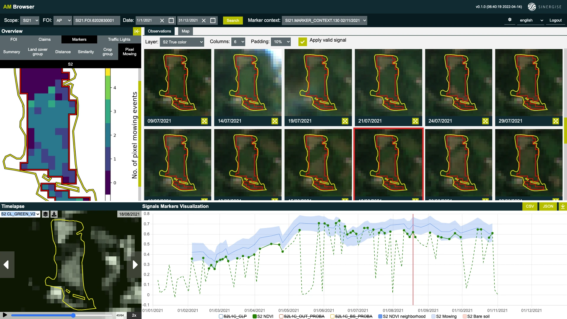
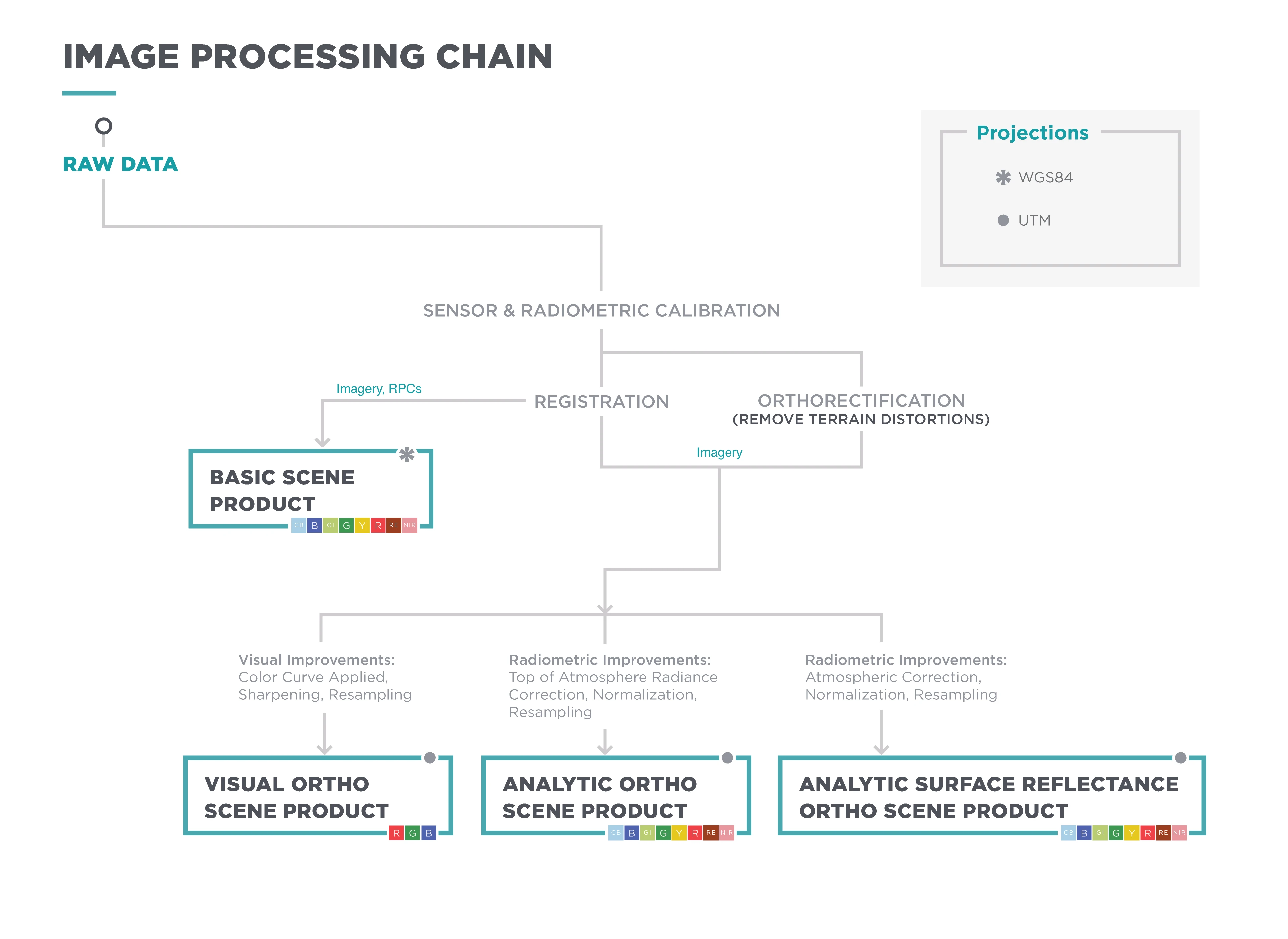
**For UDM2.0:** Percent of heavy haze values in the image. Heavy haze values represent scene content areas that contain thin low altitude clouds, higher altitude cirrus clouds, soot and dust which allow fair recognition of land cover features, but not having reliable interpretation of the radiometry or surface reflectance. | | light\_haze\_percent | int | \[0-100] | Percent of haze values in the image. Haze values represent regions of a scene with thin, filamentous clouds, soot, dust, and smoke. You can see ground objects through haze. | | shadow\_percent | int | \[0-100] | Percent of cloud shadow values in the image. Shadow values represent regions of the scene that are covered by shadows caused by clouds. | | snow\_ice\_percent | int | \[0-100] | Percent of snow and ice values in the image. Snow\_ice values represent regions of the scene that are hidden below snow and/or ice. | | visible\_percent | int | \[0-100] | Visible values represent the fraction of the scene content (excluding the portion of the image which contains blackfill) which comprises clear, light haze, shadow, snow/ice categories, and is given as a percentage ranging from zero to one hundred. | | visible\_confidence\_percent | int | \[0-100] | Average of confidence percent for clear\_percent, light\_haze\_percent, shadow\_percent and snow\_ice\_percent | \* Blackfill content refers to empty regions of a scene file that have no value ## UDM2.1 classification methodology Planet’s UDM2.1 classification approach is based on supervised machine learning techniques that use observation data from Planet satellites to train a classification model. The architecture for UDM2.1 is a modified UNET, a deep learning supervised segmentation model, that runs on 4-band (RGB-NIR) top-of-atmosphere radiance imagery. A diverse corpus containing tens of thousands of PlanetScope and SkySat images were hand-labeled to mark each pixel into one of the 5 classes noted above. The model was then trained using this labeled dataset so that it can classify new imagery into those same 5 classes. To ensure that the truth scenes dataset are representative of the global catalog of Planet images, Planet draws from a diversity of satellites, scene content, seasonality, geography and cloud types to contribute to the truth scene curation and classification process. ![](/assets/images/planetscope_udm21_production_heatmap_opacity_dots-5a0ea84f1869e7eff1117e45aaa0c1aa.webp) ![](/assets/images/skysat_udm21_production_heatmap_opacity_dots-7b21d26b247d879f7edfdc7630855b61.webp) ![](/assets/images/pelican_udm21_production_heatmap_dots-b3e8e9380dc0000c0c3e7db212a5c4cd.webp) ## Model Accuracy Planet evaluates the UDM by comparing model predictions to a sample of held-out labeled data called a validation dataset or ground truth dataset. We perform a quantitative evaluation of model accuracy by computing precision, recall and F1 metrics on a per class basis. For our validation datasets of thousands of images, we observed the following F1, precision and recall metrics: **PlanetScope** | Class | F1 | Precision | Recall | | ------------ | ----- | --------- | ------ | | Clear | 0.892 | 0.855 | 0.933 | | Snow | 0.829 | 0.836 | 0.822 | | Cloud Shadow | 0.602 | 0.597 | 0.607 | | Light Haze | 0.602 | 0.586 | 0.619 | | Heavy Haze | n/a | n/a | n/a | | Cloud | 0.948 | 0.933 | 0.964 | **Pelican** | Class | F1 | Precision | Recall | | ------------ | ----- | --------- | ------ | | Clear | 0.910 | 0.877 | 0.946 | | Snow | 0.849 | 0.827 | 0.872 | | Cloud Shadow | 0.528 | 0.494 | 0.567 | | Light Haze | 0.607 | 0.586 | 0.630 | | Heavy Haze | n/a | n/a | n/a | | Cloud | 0.962 | 0.955 | 0.970 | **SkySat** | Class | F1 | Precision | Recall | | ------------ | ----- | --------- | ------ | | Clear | 0.848 | 0.816 | 0.883 | | Snow | 0.803 | 0.780 | 0.87 | | Cloud Shadow | 0.442 | 0.391 | 0.508 | | Light Haze | 0.619 | 0.581 | 0.662 | | Heavy Haze | n/a | n/a | n/a | | Cloud | 0.924 | 0.905 | 0.944 | Planet engineering teams regularly review UDM cloud masks to identify new scenes to be added to our ground truth datasets. Additionally, customer reports of regions and specific scenes with poorly performing UDMs are an integral part of the feedback process to improve our training data and model performance. note Planet publishes imagery globally. Our goal is to ensure the highest quality in our model accuracy, but there can be anomalous behavior. If you observe poor quality, please contact your Customer Support Representative so Planet can address these issues with quarterly iterations of the model. --- Copy for LLM[View as Markdown](https://docs.planet.com/data/planet-sandbox-data/) # Planet Sandbox Data Planet Sandbox Data is a series of Data Collections that allow you to test Planet datasets. The data is made available under a [CC-BY-NC](https://creativecommons.org/licenses/by-nc/4.0/) license and is available for users with a paid subscription or [trial](https://insights.planet.com/sign-up/) accounts. Planet has made this data available for you to test out workflows, train a model, or see what a dataset looks like prior to [making a purchase](https://planet.com/pricing). We've set up data in a variety of locations to make it possible to test out different use cases. Requirements Planet Sandbox Data is available for all accounts which have processing units, both paid and trial. You can [sign up for a trial here](https://insights.planet.com/sign-up/). If you need more assistance, you can [contact our sales team](https://planet.com/contact-sales). ## Using Planet Sandbox Data To get started with using Planet Sandbox Data, you can use the following resources. ### [Explore Planet Sandbox Data via Browser →](https://insights.planet.com/analyze/browser/?tutorialIdToShow=PSD_TUTORIAL) [Quickly explore data through a web application and view pre-selected highlights.](https://insights.planet.com/analyze/browser/?tutorialIdToShow=PSD_TUTORIAL) ### [Explore Planet Sandbox Data via API →](https://github.com/planetlabs/notebooks/tree/master/jupyter-notebooks#planet-sandbox-data) [Deep dive into analysis workflows in Jupyter Notebooks from Planet's Github.](https://github.com/planetlabs/notebooks/tree/master/jupyter-notebooks#planet-sandbox-data) ## Planet Sandbox Data Locations Planet Sandbox Data is available in a subset of the [WorldStrat locations](https://worldstrat.github.io/), ranging from 25 to 200 sq km in size. The locations are spread across the world, assuring a diverse representation of different use cases. Each location has a time stack of images across a range of dates that you can use to see changes over time. ![Available locations of Planet Sandbox Data.](/data/planet-sandbox-data/world.webp) Available locations of Planet Sandbox Data. ## Available Data Collections The best way to find when and where data is available is to look at the respective sandbox data pages for each data layer in the documentation. You can find these pages below. Each page contains a map that you can use to find areas of interest and see when data is available. Select an area to find links to either open the data in the Browser or to copy the geojson to use in the APIs. [![](/data/imagery/arps/arps-2022-brazil-publish.gif)](https://docs.planet.com/data/imagery/arps/sandbox.md) ### [Analysis-Ready PlanetScope Sandbox Data](https://docs.planet.com/data/imagery/arps/sandbox.md) [![](/data/imagery/mosaics/thumbnail.webp)](https://docs.planet.com/data/imagery/mosaics/sandbox.md) ### [Mosaics Sandbox Data](https://docs.planet.com/data/imagery/mosaics/sandbox.md) [![](/data/imagery/planetscope/thumbnail.webp)](https://docs.planet.com/data/imagery/planetscope/sandbox.md) ### [PlanetScope Sandbox Data](https://docs.planet.com/data/imagery/planetscope/sandbox.md) [![](/data/imagery/skysat/thumbnail.webp)](https://docs.planet.com/data/imagery/skysat/sandbox.md) ### [SkySat Sandbox Data](https://docs.planet.com/data/imagery/skysat/sandbox.md) [![](/data/planetary-variables/forest_carbon_diligence/header-amazon.webp)](https://docs.planet.com/data/planetary-variables/forest-carbon-diligence/sandbox.md) ### [Forest Carbon Diligence Sandbox Data](https://docs.planet.com/data/planetary-variables/forest-carbon-diligence/sandbox.md) [![](/data/planetary-variables/forest_carbon_monitoring/zimbabwe_docs.webp)](https://docs.planet.com/data/planetary-variables/forest-carbon-monitoring/sandbox.md) ### [Forest Carbon Monitoring Sandbox Data](https://docs.planet.com/data/planetary-variables/forest-carbon-monitoring/sandbox.md) [![](/data/planetary-variables/land-surface-temperature/lst_thumbnail.webp)](https://docs.planet.com/data/planetary-variables/land-surface-temperature/sandbox.md) ### [Land Surface Temperature Sandbox Data](https://docs.planet.com/data/planetary-variables/land-surface-temperature/sandbox.md) [![](/data/planetary-variables/soil-water-content/swc_thumbnail.webp)](https://docs.planet.com/data/planetary-variables/soil-water-content/sandbox.md) ### [Soil Water Content Sandbox Data](https://docs.planet.com/data/planetary-variables/soil-water-content/sandbox.md) --- Copy for LLM[View as Markdown](https://docs.planet.com/data/planetary-variables/) # Planetary Variables [![](/data/planetary-variables/crop_biomass/thumbnail.webp)](https://docs.planet.com/data/planetary-variables/crop-biomass.md) ### [Crop Biomass](https://docs.planet.com/data/planetary-variables/crop-biomass.md) [![](/data/planetary-variables/field_boundaries/thumbnail.webp)](https://docs.planet.com/data/planetary-variables/field-boundaries.md) ### [Field Boundaries](https://docs.planet.com/data/planetary-variables/field-boundaries.md) [A set of polygons that represents the boundaries of agricultural fields.](https://docs.planet.com/data/planetary-variables/field-boundaries.md) [![](/data/planetary-variables/forest_carbon_diligence/header-amazon.webp)](https://docs.planet.com/data/planetary-variables/forest-carbon-diligence.md) ### [Forest Carbon Diligence](https://docs.planet.com/data/planetary-variables/forest-carbon-diligence.md) [Data on forest carbon in 30m resolution.](https://docs.planet.com/data/planetary-variables/forest-carbon-diligence.md) [![](/data/planetary-variables/forest_carbon_monitoring/zimbabwe_docs.webp)](https://docs.planet.com/data/planetary-variables/forest-carbon-monitoring.md) ### [Forest Carbon Monitoring](https://docs.planet.com/data/planetary-variables/forest-carbon-monitoring.md) [Data on forest carbon in 3m resolution.](https://docs.planet.com/data/planetary-variables/forest-carbon-monitoring.md) [![](/data/planetary-variables/land-surface-temperature/lst_thumbnail.webp)](https://docs.planet.com/data/planetary-variables/land-surface-temperature.md) ### [Land Surface Temperature](https://docs.planet.com/data/planetary-variables/land-surface-temperature.md) [![](/data/planetary-variables/soil-water-content/swc_thumbnail.webp)](https://docs.planet.com/data/planetary-variables/soil-water-content.md) ### [Soil Water Content](https://docs.planet.com/data/planetary-variables/soil-water-content.md) --- Copy for LLM[View as Markdown](https://docs.planet.com/data/planetary-variables/crop-biomass/) # Crop Biomass ![Header Thumbnail](/data/planetary-variables/crop_biomass/thumbnail.webp) Crop Biomass provides cloud-free, analysis-ready data every day. By combining optical (Sentinel-2 and PlanetScope) with radar data (Sentinel-1), this product offers users the opportunity to monitor agricultural fields, even during periods with a persistent cloud cover. Crop Biomass users get a daily raster independently of weather conditions with the data from the most updated direct observation from the day before. Each pixel has a relative measure of biomass with values that range from 0 to 1. A detailed description of Crop Biomass' methodology can be found in [Burger et al. (2024)](https://doi.org/10.3390/rs16050835). Extensive validation has been conducted on different crops. Examples of this validation can be found for grain crops in [Guillevic et al. (2024)](https://doi.org/10.1016/j.fcr.2024.109511) and for alfalfa in [Lucero et al. (2024)](https://www.mdpi.com/2072-4292/16/18/3379). ## Use Cases **Monitor crop growth and development** - You can track the growth and development of crops throughout the growing season, helping them to identify any issues early on and take appropriate action. **Detect and respond to stressors** - Frequent updates on Crop Biomass data can help you detect stressors such as pests, diseases, or nutrient deficiencies. Timely access to this information allows you to respond more quickly and effectively, minimizing potential negative impacts on crop health and yield. **Optimize inputs and interventions** - By tracking biomass dynamics, you can make better-informed decisions about the timing and application of inputs such as fertilizers and pesticides, as well as plan targeted interventions to address issues in specific areas of the field. **Improve harvest planning and efficiency** - Access to up-to-date Crop Biomass data can help you plan harvests more effectively, by identifying areas of the field with higher biomass that may require adjusted harvest strategies or equipment settings. **Estimate crop yield** - Peer-reviewed scientific article in Field Crops Research: Planet’s Biomass Proxy for monitoring aboveground agricultural biomass and estimating crop yield [Guillevic et al., 2024](https://doi.org/10.1016/j.fcr.2024.109511) ## Published Scientific Peer-Reviewed Articles: * The Biomass Proxy: Unlocking Global Agricultural Monitoring through Fusion of Sentinel-1 and Sentinel-2 [Burger et al., 2024](https://doi.org/10.3390/rs16050835) * Planet’s Biomass Proxy for monitoring aboveground agricultural biomass and estimating crop yield [Guillevic et al., 2024](https://doi.org/10.1016/j.fcr.2024.109511) ## Blog Posts * [Planet's Crop Biomass for Agriculture Monitoring and Yield Forecasting](https://medium.com/planet-stories/planets-crop-biomass-for-agriculture-monitoring-and-yield-forecasting-8211f03f14ca) * [Next Generation Agriculture Monitoring at Scale with Planet's Crop Biomass](https://www.planet.com/pulse/next-generation-agriculture-monitoring-at-scale-with-planets-crop-biomass/) ## API Access Information | API | Available | Notes | | ----------------- | --------- | ----- | | Data API | ❌ | | | Orders API | ❌ | | | Subscriptions API | ✅ | | | Analytics API | ❌ | | | Basemaps API | ❌ | | ### Subscriptions Access #### Crop Biomass 3 m Loading... #### Crop Biomass 10 m Loading... The area of interest for Crop Biomass should correspond to a single agricultural field. If the AOI of a subscription includes multiple fields, whether they contain different crops or the same crop managed differently, the resulting Crop Biomass data will not accurately reflect conditions within any specific field. For more information on the Subscriptions API and code samples, see the [API documentation](https://docs.planet.com/develop/apis/subscriptions/sources.md#planetary-variable-and-analysis-ready-source-types). ## Additional Resources [🎓Planet University](https://university.planet.com/intro-to-crop-biomass) [Learn the Crop Biomass basics with this introduction course.](https://university.planet.com/intro-to-crop-biomass) [📖Subscriptions API](https://docs.planet.com/develop/apis/subscriptions.md) [Get started with the Subscriptions API.](https://docs.planet.com/develop/apis/subscriptions.md) [📓Jupyter Notebooks](https://github.com/planetlabs/notebooks/tree/master/jupyter-notebooks/api_guides/subscriptions_api/crop_biomass) [Access Crop Biomass and create visualizations with this tutorial.](https://github.com/planetlabs/notebooks/tree/master/jupyter-notebooks/api_guides/subscriptions_api/crop_biomass) [📖EvalScripts](https://custom-scripts.sentinel-hub.com/custom-scripts/planetary-variables/crop-biomass/) [Visualize Crop Biomass and extract insights with EvalScripts.](https://custom-scripts.sentinel-hub.com/custom-scripts/planetary-variables/crop-biomass/) --- Copy for LLM[View as Markdown](https://docs.planet.com/data/planetary-variables/crop-biomass/products/) # Products ## Crop Biomass 3 m Loading... ## Crop Biomass 10 m Loading... --- Copy for LLM[View as Markdown](https://docs.planet.com/data/planetary-variables/crop-biomass/techspec/) # Technical Specification ## Overview The Crop Biomass is a fusion of microwave and optical satellite imagery, using the advantages of each to accurately estimate relative aboveground crop biomass regardless of cloud cover and at spatial resolutions of 3 and 10 meters. Crop Biomass is only available over agricultural fields. This product integrates microwave data from the European Space Agency (ESA) Sentinel-1 satellites and optical images from Sentinel-2 and PlanetScope. The output from these combined data sources is fused in an algorithm designed to provide a reliable measurement of crop biomass over agricultural areas. This is a relative measure of biomass, so each pixel value has a value of 0 (low biomass) to 1 (high biomass). The product is provided daily and in near real time (latency less than 24 hours). ## Planet's Crop Biomass: A Planetary Variable The Crop Biomass uses the vegetation signal derived from cross polarizations of microwave observations in combination with a vegetation index from Sentinel-2 and PlanetScope. The vegetation signal in the microwave region is different to the one in the optical domain. The microwave signal is a direct function of the vegetation water content, dielectric properties of the water within the vegetation, and the vegetation structure ([Ulaby et al., 1986](https://doi.org/10.1017/S0016756800015831); [Kerr et al., 1994](https://www.taylorfrancis.com/chapters/edit/10.1201/9781003424062-20/vegetation-models-observations-review-yann-kerr-jean-pierre-wigneron)). Considering the strong relationship between vegetation water content and vegetation biomass, this microwave information is, in this case, used as a biomass indicator for crops ([Vreugdenhil et al., 2018](https://doi.org/10.3390/rs10091396); [Khabbazan et al., 2019](https://doi.org/10.3390/rs11161887)). On the other hand, in optical imagery, spectral indices are used to estimate the vegetation conditions. The spectral measurements in the visible region are sensitive to the chlorophyll content, while the measurements in the near infrared are sensitive to the mesophyll structure of the leaves ([Townshend, 1993](https://catalogue.nla.gov.au/catalog/99070)). Planet offers Crop Biomass with the following features: * Daily for timely decision-making * Cloud-free for continuous and consistent feed of observations * Analysis-ready * Mid-resolution (3 and 10 m) ![](/data/planetary-variables/crop_biomass/cb_time_series.webp) *Figure 1: Measurements of Crop Biomass in eastern Mexico. The image above demonstrates both the spatial variability of the biomass for a single date (July 1, 2021), as well as the average biomass of the marked field over a timespan of four years.* ## Product Specifications | Data Resource | Crop Biomass 3 m | Crop Biomass 10 m | | --------------------- | ----------------------------------------------- | ----------------------------------------------- | | Source ID | BIOMASS-PROXY\_V5.0\_3 | BIOMASS-PROXY\_V4.0\_10 | | Unit | None (Typical Range 0 to 1) | None (Typical Range 0 to 1) | | Pixel Size | 0.000027° (±3x3 m) - EPSG:4326 | 0.000089° (±10x10 m) - EPSG:4326 | | Geographical Coverage | Global | Global | | Temporal Resolution | daily (365 observations per year) | daily (365 observations per year) | | Satellites Used | Sentinel-1, Sentinel-2, Dove (Planetscope) | Sentinel-1, Sentinel-2, Dove (Planetscope) | | Data Availability | January 2024 – present | January 2019 - present | | NRT Latency | Daily at 6am local time | Daily at 6am local time | | Archive Latency | Less than 4 hours after creating a subscription | Less than 4 hours after creating a subscription | Crop Biomass is a global product, but its geographic availability is limited in some areas between December 2021 and January 2025 due to the [failure and subsequent end of mission of Sentinel 1-B](https://www.esa.int/Applications/Observing_the_Earth/Copernicus/Sentinel-1/Mission_ends_for_Copernicus_Sentinel-1B_satellite). ### Metadata The daily GeoTIFF files include metadata that provides transparency regarding how the product is constructed. | Metadata | Description | | -------------------------------- | --------------------------------------------------------------------------------------------------------------------------------------------------------------------------------------------------------------------------------------------- | | AVERAGE\_NDVI | The average NDVI (Normalized Difference Vegetation Index) value for the date, derived from the optical data used in the product. | | CLOUD\_PROBABILITY | The cloud probability (0 to 1) from the optical imagery used. Higher values indicate cloudier conditions that may affect data quality. Derived from Sentinel-2 data and available only when a corresponding observation exists for that date. | | SURFACE\_WATER\_PROBABILITY | The probability of surface water within the field (0 to 1). Higher values indicate areas that may be affected by water or flooding. Derived from Sentinel-1 data and available only when a corresponding observation exists for that date. | | SNOW\_PROBABILITY | The probability of snow within the field (0 to 1). Higher values indicate areas that may be covered by snow. Derived from Sentinel-2 data and available only when a corresponding observation exists for that date. | | DATE\_LAST\_OPTICAL\_IMAGE\_USED | The date of the most recent optical image used in the product. This can support the understanding and interpretation of the signal, as it is an indication of the relative contribution of the optical data. | | DATE\_LAST\_S1\_IMAGE\_USED | The date of the most recent Sentinel-1 SAR image used in the product. This can support the understanding and interpretation of the signal, as it is an indication of the relative contribution of the radar data. | | LAST\_OPTICAL\_IMAGE\_SOURCE | The source of the most recent optical image used, either "PS" (PlanetScope) or "S2" (Sentinel-2). | | PERCENTAGE\_PIXELS\_MASKED | The percentage of pixels in the dataset that were masked due to issues such as cloud cover, water, snow, roads, or buildings. A value of "0.0" indicates that no pixels were masked, meaning the data is complete and unaltered. | | PRODUCT\_VERSION | The version of the product (for example, "v4" for 10 m, "v5" for 3 m), indicating the current version of the Crop Biomass product and reflecting the methodology and data processing used. | | SOFTWARE\_VERSION | The version of the biomass\_proxy software used to generate the product. Useful for debugging and tracing product lineage. | | WARNING | A warning message that appears when the field has been produced under extreme cloudy conditions. When present, it indicates that the spatial quality of the data may be impacted. | Below is a Python code snippet on how to extract the metadata from the `.tif` file of interest. ``` from osgeo import gdal def get_metadata_from_raster(file_path: str) -> dict: dataset = gdal.Open(file_path) metadata = dataset.GetMetadata() return metadata ``` ## Methodology ### Microwave data #### Sentinel-1 The Crop Biomass product leverages Sentinel-1's Synthetic Aperture Radar (SAR) data, focusing on the Cross Ratio (CR) index derived from VH (Vertical-Horizontal) and VV (Vertical-Vertical) polarizations. Sentinel-1's ability to penetrate clouds and collect data under all weather conditions makes it invaluable for agricultural monitoring, especially in regions with frequent cloud cover. The CR index highlights vegetation structure and water content while minimizing the influence of soil moisture and surface roughness, which can otherwise obscure the biomass signal. To ensure the accuracy of the CR index, the data undergoes preprocessing steps that include speckle filtering to reduce noise and orbit correction to normalize the effects of varying incidence angles and azimuth angles across different satellite passes. The resulting CR time series is then scaled to match the range of the Normalized Difference Vegetation Index (NDVI) from optical data. This scaling is crucial for fusing the radar and optical signals, allowing for a more accurate representation of crop biomass over time. ### Optical data #### Sentinel-2 Sentinel-2 provides high-resolution optical imagery, which is critical for capturing the spatial variability of crop biomass. The primary index used from Sentinel-2 is the Normalized Difference Vegetation Index (NDVI), calculated from the reflectance values in the red (Band 4) and near-infrared (Band 8) regions of the electromagnetic spectrum. NDVI is widely recognized for its sensitivity to chlorophyll content and vegetation health, making it an excellent proxy for biomass. Sentinel-2 data is preprocessed to remove clouds, snow, and any man-made structures such as green houses, roads, or buildings. To address gaps in temporal coverage due to clouds or infrequent satellite passes, a dynamic interpolation method is used, extrapolating partially cloud-covered images by referencing the most recent cloud-free image. This approach ensures a continuous time series of NDVI values. #### PlanetScope PlanetScope imagery, with its higher revisit frequency, complements Sentinel-2 by filling in temporal gaps. This additional data source is especially valuable in regions with persistent cloud cover or during critical growing periods when timely biomass data is essential. The integration of PlanetScope data enhances the spatial and temporal resolution of the Crop Biomass product, making it more robust and reliable. ### Data Inputs Table 1: List of inputs for Crop Biomass production | Product | Description | | ------------------------------------- | --------------------------------------------------------------------------------------------------------------------------------------------------------------------------------------------------------------------------------------------------------------------------------------------------------------------------------------------------------------------------------------------------------------------------------------------------------------------------------------------------------------------------------------------------------------------------------------------------------------------------------------------------------------------------------------------------------------------------------------------------------------------------------------------------------------------------------- | | Radar backscatter | C-Band Synthetic Aperture Radar (SAR) data from the Sentinel-1A Level-1 ground range detected (GRD) product, in the IW mode (downloaded with the SentinelHub Asynchronous API). The product consists of focused SAR data that has been detected, multi-looked, and projected to ground range using the Earth ellipsoid model WGS84. This GRD product has a pixel spacing of 10 x 10 meters. Before December 2021, Sentinel-1B was also in orbit and is part of the archive data for CB. Detailed information is available [here](https://sentiwiki.copernicus.eu/web/document-library#Product-Definition-and-Specification). | | Reflectances Red and NIR bands (10 m) | Sentinel-2 Level-1C reflectances (downloaded with the SentinelHub Asynchronous API) for the two bands: red (around 665 nm) and NIR (near-infrared around 842 nm). This product provides orthorectified (geometric ortho-correction taking into account a DEM) Top Of Atmosphere reflectance (more details [here](https://sentiwiki.copernicus.eu/web/s2-processing)). The cloud masking is performed in-house using [S2Cloudless](https://www.pythonfmask.org/en/latest/). Detailed information is available [here](https://sentiwiki.copernicus.eu/web/document-library#Product-Specification-Documents). | | Reflectances Red and NIR bands (3 m) | PlanetScope Ortho Scene product provides orthorectified, multispectral imagery from the PlanetScope constellation, for the red (around 665 nm) and NIR (near-infrared around 865 nm) bands. The imagery is collected by the SuperDove satellites at a 3-meter ground sample distance (GSD) at nadir and has a pixel size of approximately 3 meters after orthorectification. The product is processed to remove geometric distortions, using ground control points (GCPs) and digital elevation models (DEMs), ensuring a positional accuracy of less than 10 meters RMSE at the 90th percentile. The [UDM 2.1](https://docs.planet.com/data/imagery/udm.md) cloudmask is applied to the product. Detailed information is available [here](https://assets.planet.com/docs/Planet_PSScene_Imagery_Product_Spec_letter_screen.pdf). | | Field Boundaries | Geospatial boundaries of agricultural fields, used to define the areas for biomass estimation. These boundaries are essential for accurate data fusion, as the product works at field-level. The boundaries are provided by the client in a GeoJSON format. | ### Data Fusion and Scaling The core innovation of the Crop Biomass product lies in its data fusion methodology, which integrates the temporally consistent radar signal from Sentinel-1 with the spatially detailed optical signal from Sentinel-2 and PlanetScope. You can read more about the methodology in the published paper: *The Biomass Proxy: Unlocking Global Agricultural Monitoring through Fusion of Sentinel-1 and Sentinel-2* ([Burger et al., 2024](https://doi.org/10.3390/rs16050835)). This fusion process is conducted in two main steps: 1. **Temporal Fusion**: The CR and NDVI time series are combined at the field level using a dynamic weighting strategy. This strategy assigns more weight to the most reliable and recent observations, ensuring that the temporal evolution of the biomass signal is accurately captured. 2. **Spatial Fusion**: Once the temporal signal is established, it is downscaled to a 10-meter resolution by integrating the spatial patterns observed in the optical data. This step involves applying a spatial weighting function that accounts for the variations in both radar and optical signals across the field, resulting in a high-resolution biomass map that combines the strengths of both data sources. ## Data Quality ### Validation We have rigorously evaluated the CB against both field measurements and other remote sensing products, such as NDVI. Given the wide range of potential use cases—such as crop monitoring, event detection, and yield forecasting—the validation process is an ongoing effort. To illustrate its value, we will briefly explore two common use cases: crop monitoring and yield forecasting. NDVI is commonly used for crop monitoring as it effectively measures plant greenness. However, many widely cultivated crops change color as they approach the final stages of growth before harvest. For instance, barley (or other grains) and canola exhibit significant differences when comparing CB with NDVI. As barley ripens, it changes color from green to light brown, and canola’s yellow flowers reflect more red light, leading to a decrease in NDVI values. In contrast, the CB product accounts for the actual biomass of the crops, enabling a more accurate estimation of the harvest date. This capability to measure biomass directly distinguishes CB from NDVI, particularly in assessing crop maturity and planning harvests. ![](/data/planetary-variables/crop_biomass/cb_timeseries_validation.webp) *Figure 2. The Crop Biomass and NDVI time series for barley and canola, demonstrating different features associated with color changes.* ([Burger et al., 2024](https://doi.org/10.3390/rs16050835)) You can read more about the yield-related validation in the published paper *Planet’s Biomass Proxy for monitoring aboveground agricultural biomass and estimating crop yield* ([Guillevic et al., 2024](https://doi.org/10.1016/j.fcr.2024.109511)) In the validation paper, you will find a comprehensive analysis of the product's performance in yield estimation for corn, wheat, and soybean—some of the most widely cultivated crops globally. The product's performance is assessed by correlating either the maximum or an aggregated value of biomass to the yield. Data points were collected from several fields in Mead, Nebraska, and Kellogg, Michigan. This analysis demonstrates both the Crop Biomass' ability to forecast yield before the end of the growing season, as well as to capture the intra-field variability of the biomass. ![](/data/planetary-variables/crop_biomass/cb_yield_validation.webp) *Figure 3. Relationships between crop yield and three different yield indicators based on time series of Biomass Proxy (BP): the maximum value of BP through the crop season (a), the mean values of BP from crop emergence to BP max (b) and the mean value of BP over growing-degree-days (GDD) -based integration periods.*([Guillevic et al., 2024](https://doi.org/10.1016/j.fcr.2024.109511)) ### Quality Control Quality control of the Crop Biomass product is conducted on two levels: within the algorithm itself and through metadata. The algorithm ensures quality in several ways, beginning with the quality of the input data. Each observation is assigned a quality factor based on the number of valid pixels (for example, those without clouds, water, snow, roads, buildings, etc.) and this factor decreases over time. This mechanism, along with extensive preprocessing of all input data, ensures that the product remains as up-to-date and accurate as possible. See the [Metadata description](https://docs.planet.com/data/planetary-variables/crop-biomass/products.md#Metadata) for more details. ### Limitations The following are some key limitations that need to be considered: * Sentinel-1 signal is not NDVI: The agricultural market is “trained” on NDVI. The cross-ratio is an index derived from different Sentinel-1 polarizations. The differences in behavior between radar-based and optical index must be considered when offering this product. * Behavior in pastures, grasslands and other low-growing vegetation: Crop Biomass is generally not recommended for pastures, grasslands, or other low-growing vegetation. The product relies heavily on Sentinel-1 C-band radar. When vegetation is low to the ground, the radar signal penetrates completely to the soil. As a result, the signal becomes dominated by soil moisture rather than actual vegetative biomass. This creates unreliable, artificial "spikes" in Crop Biomass values. * Possible changes upon re-request: There may be relatively small changes in Crop Biomass values when re-requesting data for the same field and date. This is due to [subtle changes in the underlying PlanetScope data](https://docs.planet.com/data/imagery/planetscope.md#planetscope-publishing-lifecycle) that may occur as items are republished with quality improvements. ## Frequently Asked Questions #### Will the Crop Biomass PV work for smallholder farms? We tested the product in different regions with small-scale fields. While the data shows consistency up to 0.2 hectares, its quality will also depend on the presence of mixed crops. #### Is there demo data available? Demo data should be prepared by pre-sales on-demand. #### Can customers use the Crop Biomass in Sentinel Hub? Yes, subscriptions can be generated and visualized in the EO Browser. Also, subscriptions can be hosted in Sentinel Hub through Planet’s API. #### Does Crop Biomass work for orchards and vineyards? We tested our data in different crops including orchards and vineyards. As mentioned above, the behavior of Sentinel-1 derived indices is different from the ones from optical-derived sources. Our team can share information with prospective customers that are crop-specific. #### How can I extract the metadata? The simplest way to inspect the metadata is with the command line: ``` gdalinfo your_tif_file.tif ``` This will show a list of specifics of the file, such as the coordinate reference system, the pixel size, the extent, and the metadata. Alternatively, you can also do this in Python as shown in [the quality control section](#quality-control). --- Copy for LLM[View as Markdown](https://docs.planet.com/data/planetary-variables/field-boundaries/) # Field Boundaries ![Header Thumbnail](/data/planetary-variables/field_boundaries/thumbnail.webp) Field Boundaries is an enabling Planetary Variable that provides critical infrastructure required to answer many of the larger scale questions about agriculture production. Field delineation is the process of automatically tracing the boundaries of agricultural parcels from satellite or aerial imagery. An agricultural parcel is a spatially homogeneous land unit used for agricultural purposes, where a single crop is grown. The result of field delineation is field boundaries, a set of closed vector polygons marking the extent of each agricultural parcel. Such polygons are the input to a multitude of applications, ranging from the management of agricultural resources, such as Area Monitoring, precision farming, to the estimation of damages to crop yield due to natural disasters like drought and floods, and human-made disasters like war. Automatic estimation of parcels with high fidelity in a timely manner allows to characterize changes of agricultural landscapes due to agricultural practices and climate change consequences. ## Use Cases * Yield estimation * Agricultural Monitoring and Food Security * Commodity Trading * Sustainable Agriculture Monitoring (including CAP and EUDR) * Supply Chain Monitoring * Benchmarking * Product Supply Forecasting * Biofuels * Environmental Impact Assessment * Proof of Permit and Regulatory Compliance * Risk Assessment * Agricultural Insurance (underwriting, pricing, claims validation) * E\&R (Scientific publications and research grants) * Field Isolation ## API Access Information | API | Available | Notes | | ----------------- | --------- | ----- | | Data API | ❌ | | | Orders API | ❌ | | | Subscriptions API | ✅ | | | Analytics API | ❌ | | | Basemaps API | ❌ | | ### Subscriptions Access Loading... Each request made using the Subscriptions API, delivers a GeoPackage that includes field boundaries for the specified TOI and AOI. Polygons with an area lower than 50 sqm are removed from the output. Polygons with Maximum Inscribed Circle Diameter (MICD) lower than 30 m are flagged as unreliable. For more information on the Subscriptions API and code samples, refer to the [API documentation](https://docs.planet.com/develop/apis/subscriptions/sources.md#planetary-variable-and-analysis-ready-source-types). ## Additional Resources [📖Subscriptions API Guide](https://docs.planet.com/develop/apis/subscriptions.md) [Learn how to work with Planet subscriptions API through the Quickstart guide.](https://docs.planet.com/develop/apis/subscriptions.md) [🎓Planet University](https://university.planet.com/intro-to-field-boundaries) [Explore video tutorials about Field Boundaries](https://university.planet.com/intro-to-field-boundaries) [📰Field Delineation Release](https://medium.com/sentinel-hub/automatic-field-delineation-new-release-1c2938399f0) [Research and development that led to the new version of Planet Field Boundaries.](https://medium.com/sentinel-hub/automatic-field-delineation-new-release-1c2938399f0) [📰AI4Boundaries & EuroCrops](https://medium.com/sentinel-hub/utility-of-ai4boundaries-and-eurocrops-as-training-datasets-for-field-delineation-ff514471d067) [Analysis of training datasets for field delineation.](https://medium.com/sentinel-hub/utility-of-ai4boundaries-and-eurocrops-as-training-datasets-for-field-delineation-ff514471d067) --- Copy for LLM[View as Markdown](https://docs.planet.com/data/planetary-variables/field-boundaries/products/) # Products ## Field Boundaries Loading... ### Assets Loading... ### Attributes More details are available in the [Technical Specification](https://docs.planet.com/data/planetary-variables/field-boundaries/techspec.md#attributes-description) --- Copy for LLM[View as Markdown](https://docs.planet.com/data/planetary-variables/field-boundaries/techspec/) # Technical Specification ## Overview ## Planet's Field Boundaries: A Planetary Variable The Field Boundaries (FB) dataset is a Planetary Variable™ containing a set of polygons that represents the boundaries of agricultural fields. Field delineation is the process that generates FBs by automatically tracing the boundaries of agricultural fields from Sentinel-2 satellite imagery with 10 m spatial resolution. An agricultural field is a spatially homogeneous land unit utilized for agricultural purposes, where a single crop is grown. Planet’s Field Boundaries algorithm leverages the similarity of spatial, spectral, and temporal properties of pixels belonging to the same field. A deep neural network based on the popular U-net architecture is used to estimate the field’s extent, boundary, and the distance of the segmented image pixels to the boundary. The estimated probability images are then combined into a single pseudo-probability image representing the extent of the fields. In post-processing, the image prediction is converted into vector format, where each polygon represents the extent of a homogeneous agricultural field. The result is a set of closed vector polygons marking the extent of each agricultural field. Additionally, a quality assessment attribute is computed for each estimated FB polygon. ## Inputs For the specified TOI, Sentinel-2 satellite images are downloaded as well as the cloud masks. Sentinel-2 bands at 10 m spatial resolution are used, specifically B02, B03, B04, and B08. The dataMask band is used for handling pixels with no-data. No-data pixels are all pixels which lie outside of the area of interest, all pixels for which no source data was found, and all pixels for which source data was found but are invalid. Additionally, utilized alongside the native Sentinel-2 bands is s2cloudless, a machine learning algorithm for computing cloud masks and probabilities on Sentinel-2 imagery, sampled at 160 m resolution. They are available as Sentinel-2 bands named CLP (cloud probabilities) and CLM (cloud masks). ## Field Boundaries Product Information is available in the [Product Page](https://docs.planet.com/data/planetary-variables/field-boundaries/products.md) ### Attributes Description To facilitate characterization and interpretability of the resulting polygons, some attributes are added and a quality assessment attribute is computed for each estimated FB polygon. The attributes are listed in the [table](https://docs.planet.com/data/planetary-variables/field-boundaries/products.md#attributes) and details on these are provided below. **Polygon ID** To facilitate downstream usage and indexing of the FB polygons, a unique integer identifier is assigned to each polygon. Uniqueness of the identifier is guaranteed only within a delivered GeoPackage file for a subscribed AOI. The same identifier will correspond to different polygons for different deliveries of the same AOI, or for different AOIs. **Area** The area of the polygon in hectares is included as an attribute (1 ha is 10,000 sqm). The area is computed before conversion to the common WGS84 coordinate reference system. **Maximum Inscribed Circle Diameter (MICD)** While the polygon area is a general descriptor for the size of a polygon, it carries no information about its shape. While evaluating and validating the FB product, it was observed that the shape of the polygon correlates more with the performance of the algorithm, rather than its size only. This has to do with the limitations in spatial resolution of the input imagery, which affect the minimum side (for example, height or width) of the polygon that can be detected. A very narrow but long polygon can have a large value of area, but nevertheless cannot be reliably detected by the algorithm due to its narrower side. MICD was identified to be a suitable metric for estimating the polygon width. The maximum inscribed circle is the largest circle which can be inscribed within the polygon, see Figure 2. MICD is added as an attribute, and used to flag polygons of uncertain accuracy. ![](/data/planetary-variables/field_boundaries/fb_polygons_micd.webp) *Figure 1: Illustration of an example of MICD for three different polygons. The central polygon is unlikely to be correctly delineated despite its non-negligible area, due its width, which is smaller than the Sentinel-2 spatial resolution. This highlights that area is not a good proxy for performance of the algorithm.* **Circumference-Area ratio (CA ratio)** A normalized Circumference-Area ratio is added to each polygon to additionally describe its shape. The CA ratio can be used in conjunction to the Area and MICD attributes to identify polygons of circular shape (for example, with CA ratio close to 0), of squared shape (for example, with CA ratio around 1), or of more irregular shape, having CA ratio larger than 10. Examples of CA ratio are shown in Figure 3. ![](/data/planetary-variables/field_boundaries/fb_polygons_ca_ratio.webp) *Figure 2: Examples of polygons with different CA ratios: 0,08 (left), 1,05 (middle) and 45,47 (right).* **Quality Assessment Attribute** A quality assessment (QA) attribute denotes polygons with known limitations. The attribute is an unsigned integer. The values presented in the table below are provided for the current version of the FB product. Table 4: Values and their description of the QA attribute. | QA Value | Description | | -------- | -------------------------------------------------------------------------------------------------------------------------------------------------- | | 0 | Polygons for which the validation scores are representative, for example with MICD > 30 m. | | 1 | Polygons for which the validation scores are not representative, for example with MICD < 30 m. The quality for these polygons is likely to be low. | | 2 | Polygons that are intersecting the border of the data availability grid. | The provided example illustrates four types of polygons. Polygons outside of the AOI are removed from the output. The remaining ones (depicted with solid and diagonal fill) intersect with the AOI and are therefore kept in the output. Polygons that are intersecting the border of the data availability grid are also kept in the output and are assigned a value of qa==2. We suggest removing such polygons from further analyses, as they only partially cover the underlying field. ![](/data/planetary-variables/field_boundaries/fb_da_grid.webp) *Figure 3: Example of four types of polygons.* ### Data Availability The additional output of the FB product includes a data availability map - a vector file suffixed \_da. This map consists of a grid, representing the customer's AOI split during processing. Each grid cell has an attribute called ‘has\_valid\_observations.’ When this attribute is set to ‘false,’ it indicates that there were no valid Sentinel-2 observations available for the TOI defined by the customer. Consequently, the model failed to predict field boundaries within that specific grid cell. On the other hand, when ‘has\_valid\_observations’ is set to ‘true,’ it indicates that valid observations were available for the specific grid cell, leading to the successful production of field boundaries. Table 6: Data availability map specifications. | Attribute | Description | | ------------------------ | ------------------------------------- | | Type of product | Vector | | Input data source | Sentinel-2 (10 m) | | Input data time interval | Output based on 1 month of data (TOI) | | Attribute | has\_valid\_observations | ## Delivery The output of FB is a GeoPackage (GPKG), which contains a vector data layer of delineated polygons representing fields within the chosen Area of Interest (AOI). Moreover, Planet provides a data availability map as an additional output. FB is delivered through the Subscription API into a designated storage cloud bucket. Subsequently, the customer receives a notification regarding the availability of the data. Table 7: Vector properties of FB outputs. ## Methodology Planet carries out the following steps to produce boundaries of the agricultural fields: * split the AOI into a grid to parallelize and speed up processing * retrieve remote sensing imagery for the time period of interest * spatially coregister the multiple images * inference of the pre-trained deep learning model on the input imagery, obtaining pseudo-probability maps of field boundary estimates * post-processing of the pseudo-probabilities to obtain a single vector file of merged agricultural field boundaries * compute attributes ![](/data/planetary-variables/field_boundaries/fb_production_pipeline.webp) *Figure 4: Production pipeline.* The AOI is split into a regular grid, which allows massive parallelization of the processing. For each grid cell, Planet performs data download, pre-processing, model prediction and post-processing. Predictions across all grid cells are merged in a complete map during the final stages of the process. Accurate field delineation requires clear-sky observations. For the selected TOI, satellite images, as well as cloud and no-data masks are downloaded for each grid cell using Batch API. Estimates of cloud coverage are produced for each grid cell. If cloudless scenes exist (for example, with a cloud coverage below 10%), only these are considered to generate a consensus. If no cloudless scenes are available, a consensus is generated using all scenes in the grid cell, by only considering pixels not covered by clouds. This is performed in order to ensure that clouds and related artifacts do not affect the estimation of boundaries. When no valid Sentinel-2 observations are available for a specific grid cell during the TOI defined by the customer, the model fails to predict field boundaries within that specific grid cell. In the additional output Data Availability map these grid cells have the value of the has\_valid\_observations attribute set to false. Co-registration of the input satellite time-series within a grid cell is applied to reduce frame-to-frame misalignments, and therefore to reduce noise when creating a temporal consensus. Each input Sentinel-2 band is normalized using statistics pre-computed over a large area. Following normalization, a pretrained U-net network, inspired by [Waldner and Diakogiannis (2020)](https://doi.org/10.1016/j.rse.2020.111741), is employed to infer extent, boundary and distance to boundary of each detected agricultural field for each input observation of the time-series. The U-net network has been trained on pre-processed data from the EuroCrops dataset in a separate training phase. As the model is not trained on temporal data, and significant differences may exist in predictions made between different observations, different temporal predictions are temporally merged into a single prediction. The resulting image has continuous values that can be treated as a level set function, and can therefore be thresholded to obtain smooth contours. In the final step, Planet merges vector predictions over grid cells (and over UTM zones), resolving the duplication of vectors in overlapping regions of neighboring grid cells. To correctly produce field boundaries, an assumption about the dimensional limits of the polygons needs to be made. Polygons of area lower than 50 sqm, for example half the size of a Sentinel-2 pixel, are removed from the database. These are noisy predictions mostly due to post-processing. Very large and very long polygons that spread over large distances may also present an issue for producing accurate results. Maximum Inscribed Circle Diameter (MICD) is the largest circle which can be inscribed within the polygon, and is an intuitive proxy for the width of a field. We mark polygons as unreliable (qa value 1) in Quality Assessment attribute if their MICD is less than 30 meters, which essentially means their minimum/shorter side is less than 30 meters. For each estimated polygon, Planet computes attributes that facilitate the characterization and analysis of the results for downstream applications. The provided attributes for each polygon are: an ID, area in hectares, MICD, which is used to compute the Quality Assessment attribute, and the Circumference-Area ratio. These attributes can be combined to filter polygons of lower quality by the end user. ### Validation We evaluated the FB product extensively on the largest source of reference data in Europe, for example, EuroCrops dataset. The dataset is based on GSAA polygons, which have known quality limitations (described in [Utility of AI4Boundaries and EuroCrops as training datasets for field delineation](https://medium.com/sentinel-hub/utility-of-ai4boundaries-and-eurocrops-as-training-datasets-for-field-delineation-ff514471d067) blog post), leading to under-estimation of the delineation performance. However, such a dataset allows us to evaluate the algorithm on a diverse set of samples, in terms of sizes, shapes and semantic definitions. As can be expected due to the limitations of the spatial resolution of the input imagery, the performance increases as the size of the fields increases, with median IoU scores greater than 0.8 for fields having minimum side larger than 150m, reaching a IoU up to 0.98 for for fields with minimum side larger than 240m. Check out the [validation report](https://planet.widen.net/s/wbbfbnznlv/planet-whitepaper-fieldboundariesvalidationreport-letter) for more detailed information. ### Limitations When assessing the FB dataset it is crucial to consider the following points about the model: 1. TRAINED FOR DELINEATING ARABLE LAND: the deep learning model was trained to delineate arable land; 2. TRAINING DATA SOURCE: The model was trained on GeoSpatial Aid Application (GSAA) data, annual crop declarations made by European farmers for Common Agricultural Policy (CAP) area-based support measures. This data is not always aligned with boundaries seen on the ground at a certain acquisition and can be incomplete and outdated, since national paying agencies are not yet obliged to maintain such a dataset; 3. RESOLUTION LIMITATION: Predictions are based on Sentinel-2 imagery with a 10 m spatial resolution. The following limitations have been identified: * The majority of the EuroCrops data covers central and northern European countries, therefore the model has been primarily exposed to, and trained on, data from these regions. * The model was trained to delineate agricultural areas (for example, annual crops), therefore the quality of field boundaries over grassland (pastures, meadows) and areas with permanent crops (orchards, vineyards, olive groves) is lower. * The FBs are constructed from cloud-free observations over the AOI from the time interval of one month. In some cases over cloudy areas the single-month approach might not produce fields over some areas, as shown in the availability maps. A vector file containing a data availability map that highlights areas lacking valid Sentinel-2 observations for field boundary prediction is provided. It assists customers in identifying data gaps. * The performance is less favorable in arid regions, particularly evident in Mediterranean countries, attributed to the challenge of less distinct field boundaries in arid landscapes, and a lack of training samples in such areas. * Due to the model being based on Sentinel-2 imagery with a 10 m resolution, predictions for fields with MICD less than 30 m may be of low quality or, in some cases, may be missing. For this reason, a data quality flag will identify such polygons. * Some resulting field boundaries might be joined at either end of the field as a result of the super-resolution layers. This generates larger field boundaries that are however not fully disconnected. * Predictions might present holes, which in some cases can correspond to actual non-arable land objects, such as trees, large boulders or wind mills, but can also in some cases correspond to uncertain boundaries not completely detected. ![](/data/planetary-variables/field_boundaries/fb_polygons_holes.webp) *Figure 5: Example of undesired holes due to uncertain boundaries on the left, while the right figure shows holes that correctly detect non-arable land objects.* * The FB dataset might not be suitable for variable rate application, as the polygons can not compare to digitized polygons in terms of quality and size, due to limitations of the spatial resolution of the input Sentinel-2 imagery. They tend to be systematically smaller than the ground truth field boundaries, and they exhibit rounded corners. ## Frequently Asked Questions #### What imagery is used to create the Field Boundaries PV and why? The first version of Field Boundaries uses data from Sentinel-2 with 10 m resolution. Historically, FBs were created by Sinergise within an European Commission funded research project on Sentinel-2, and the results for large fields are reliable even with using Sentinel-2 data. #### Which TOI is recommended? We generally suggest choosing a month that represents the early growing phase of crops, such as May or June for the northern hemisphere. #### Does the Field Boundary PV work for smallholder farms? V1 of the Field Boundary PV is not well suited to smallholder farms due to the 10m resolution of the Sentinel data that was used to create this first version of the product. #### Field Boundaries fault towards underestimation of area versus overestimation. How much area is underestimated on average? There is high variability depending on the shape and size of the polygons, but on average around 10 %. --- Copy for LLM[View as Markdown](https://docs.planet.com/data/planetary-variables/forest-carbon-diligence/) # Forest Carbon Diligence ![Header Thumbnail](/data/planetary-variables/forest_carbon_diligence/header-amazon.webp) The Forest Carbon Diligence product is composed of a bundle of data resources: Canopy Height, Canopy Cover, and Aboveground Live Carbon at 30-meter spatial resolution. These data resources are produced annually over the entire landmass of the Earth (between 75° N and 60° S). We use an extensive library of airborne LiDAR to train deep learning models to predict canopy height and canopy cover from satellite imagery. We use these predictions paired with 11 million spaceborne lidar (GEDI) footprints to train a model to estimate aboveground live carbon. The archive currently extends back to 2013. See the Technical Specification for more details. ## Basic Facts | **Property** | **Info** | | ---------------------- | --------------------------------------------------------------------------------------------------------------------------------------------------------------- | | Spatial resolution | 30 m | | Sensor/Input Data | Airborne LiDAR, LiDAR (GEDI), Landsat 8, Sentinel 2, ALOS-PALSAR-2, Wood density, Digital Elevation Model (DEM) | | Revisit time | Annual | | Spatial coverage | Global | | Data availability | Global since 2013 | | Available measurements | Canopy Height, Canopy Cover, and Aboveground Live Carbon | | Common usage/purpose | Planet's Forest Carbon Diligence products quantify—globally and annually—how much carbon is stored in trees, the area occupied by trees, and how tall they are. | Forest Carbon Diligence Data Releases New Forest Carbon Diligence data is released mid year, depending on the release of [ALOS PALSAR data](https://www.eorc.jaxa.jp/ALOS/en/dataset/fnf_e.htm). See the [changelog](https://docs.planet.com/develop/changelog.md) for the latest releases and to stay notified of new releases. ## Use Cases **Forest Carbon Projects** - Forest Carbon Diligence enables the quantification of carbon stocks and forest area over time to accurately quantify losses and gains. The accuracy is comparable to airborne approaches but the data is orders of magnitude less expensive while being globally available, providing a cost-effective solution for comprehensive monitoring. The high precision, accuracy, and granularity offered by the Forest Carbon Diligence provides an objective foundation for identifying and implementing improvements in carbon initiatives. **Deforestation Monitoring for Supply Chains** - Forest Carbon Diligence data provides comprehensive monitoring by quantifying deforestation on a high-frequency cadence. Stakeholders can report on their supply chains to forests globally with unprecedented granularity and confidence. In the context of the EU Deforestation Regulation (EUDR), the Forest Carbon Diligence dataset offers more precise data, aligning with the regulation’s focus on defining deforestation boundaries and providing crucial context regarding forest degradation and carbon loss. ## API Access Information | API | Available | Notes | | ----------------- | --------- | ----- | | Data API | ❌ | | | Orders API | ❌ | | | Subscriptions API | ✅ | | | Analytics API | ❌ | | | Basemaps API | ❌ | | ### Subscriptions Access #### Canopy Height 30m Loading... #### Canopy Cover 30m Loading... #### Aboveground Carbon Density 30m Loading... For each request you make using the Subscriptions API, you'll get a dataset that includes forest carbon estimations for the specified TOI and AOI. For more information on the Subscriptions API and code samples, see the [API documentation](https://docs.planet.com/develop/apis/subscriptions/sources.md#planetary-variable-and-analysis-ready-source-types). ### Subscriptions Time of Interest The table below provides an example of the temporal periods and the date tags associated with Forest Carbon Diligence data. When creating a subscription, the 'start\_time' must be set to the date tag or earlier, while the 'end\_time' must be set to a date after the date tag. | **Year** | **Start** | **End** | **Date Tag** | | -------- | ---------- | ---------- | -------------------- | | 2023 | 2023-01-01 | 2023-12-31 | 2023-01-01T00:00:00Z | ## Example Workflows Below are links to a series of Python workflows that highlight ways you can access and analyze the Forest Carbon Diligence data. ## Analyze Historical Trends Without Downloading Data This workflow walks you through how to create a subscription with the Subscriptions API, deliver the data to a cloud bucket, and then retrieve and analyze the data directly from the cloud (for example, without having to download it locally). [Go to Guide →](https://docs.planet.com/guides/analyze-historical-forest-carbon.md) ## Mapping Forest Cover Change via Planet Insights Platform This workflow demonstrates how to map changes in forest cover between two dates based on the Forest Carbon Diligence product using the Processing API. [Go to Guide →](https://github.com/planetlabs/notebooks/blob/master/jupyter-notebooks/use_cases/forest_carbon_dilligence/pv-forest-change.ipynb) ## Additional Resources [📖Technical Specification](https://docs.planet.com/data/planetary-variables/forest-carbon-diligence/techspec.md) [Get the details in the Forest Carbon Diligence Technical Specification](https://docs.planet.com/data/planetary-variables/forest-carbon-diligence/techspec.md) [🎓Planet University](https://university.planet.com/intro-to-forest-carbon-diligence-and-monitoring) [Get Started with Planet’s Forest Carbon Planetary Variable product for: global tree height, canopy cover and carbon raster.](https://university.planet.com/intro-to-forest-carbon-diligence-and-monitoring) [📓Guides](https://docs.planet.com/guides.md) [Visit our Guides page to find related Jupyter Notebooks for hands-on learning.](https://docs.planet.com/guides.md) [📚APIs](https://docs.planet.com/develop/apis/subscriptions.md) [Learn more about the Planet Subscriptions API to obtain Forest Carbon data.](https://docs.planet.com/develop/apis/subscriptions.md) --- Copy for LLM[View as Markdown](https://docs.planet.com/data/planetary-variables/forest-carbon-diligence/products/) # Products Below you will find a list of Data Resources available for the Forest Carbon Diligence product. Each Data Resource has a series of associated Data Assets. We are continuously working to improve the product, and periodically release new versions. We provide access to older versions of our products, but only produce data using the latest version at new timesteps. We recommend using the latest product version and reviewing the [version history in the changelog](https://docs.planet.com/develop/changelog.md?tag=forestCarbonDiligence) associated with each release. ## Canopy Height 30m Loading... ## Canopy Cover 30m Loading... ## Aboveground Carbon Density 30m Loading... --- Copy for LLM[View as Markdown](https://docs.planet.com/data/planetary-variables/forest-carbon-diligence/sandbox/) # Forest Carbon Diligence Sandbox Data This Planet Sandbox Data collection for Forest Carbon Diligence provides sample data over specific areas and times of interest. The data is available to paid and trial accounts that include processing units and is available under the CC-BY-NC license. Learn more about [Planet Sandbox Data](https://docs.planet.com/data/planet-sandbox-data.md). ## Data Collections Metadata | Source ID | Collection Name | Collection ID | Time Range | | ---------------------------------------- | ----------------------------------------------- | ----------------------------------------- | ----------------------- | | CANOPY\_HEIGHT\_v1.1.0\_30 | Planet Sandbox Data - PV FCD Canopy Height | BYOC-f3312c82-edea-42a1-8c9d-ada86ddcc857 | 2013-01-01 - 2017-01-01 | | CANOPY\_COVER\_v1.1.0\_30 | Planet Sandbox Data - PV FCD Canopy Cover | BYOC-e3d2a21c-cb75-4311-86ac-024385c85b9c | 2013-01-01 - 2017-01-01 | | ABOVEGROUND\_CARBON\_DENSITY\_v1.1.0\_30 | Planet Sandbox Data - PV FCD Aboveground Carbon | BYOC-cc31cada-80d8-46fe-a746-43ac2f87b5da | 2013-01-01 - 2017-01-01 | ## Planet Sandbox Data Areas This collection includes 4 sandbox regions. Download the GeoJSON file below the map for exact polygon boundaries. View all 4 regions | Location | Area (km²) | Time Range | Center (lat, lon) | | ----------------------------------------------- | ---------- | ----------------------- | ----------------- | | Pará, North Region, Brazil | 568 | 2015-01-01 – 2017-01-01 | -6.77, -52.37 | | Iowa, United States | 581 | 2015-01-01 – 2017-01-01 | 41.30, -93.95 | | Western Australia, Australia | 587 | 2015-01-01 – 2017-01-01 | -31.92, 116.15 | | Nouvelle-Aquitaine, Metropolitan France, France | 599 | 2015-01-01 – 2017-01-01 | 44.73, -0.68 | [Download GeoJSON](https://docs.planet.com/data/planetary-variables/forest_carbon_diligence/polygons.geojson) ## Highlights [![Bordeaux, France](/data/planetary-variables/forest_carbon_diligence/FCD_FRA.webp)](https://insights.planet.com/analyze/browser/?zoom=12\&lat=44.7345\&lng=-0.676\&themeId=PLANET_SANDBOX\&visualizationUrl=https%3A%2F%2Fservices.sentinel-hub.com%2Fogc%2Fwms%2Ff006c031-60da-4262-bdf7-6fc4f1532d13\&datasetId=cc31cada-80d8-46fe-a746-43ac2f87b5da\&fromTime=2017-01-01T00%3A00%3A00.000Z\&toTime=2017-01-01T23%3A59%3A59.999Z\&layerId=ABOVEGROUND-CARBON-DENSITY\&demSource3D=%22MAPZEN%22) Bordeaux, France 2015-01-01 to 2017-01-01
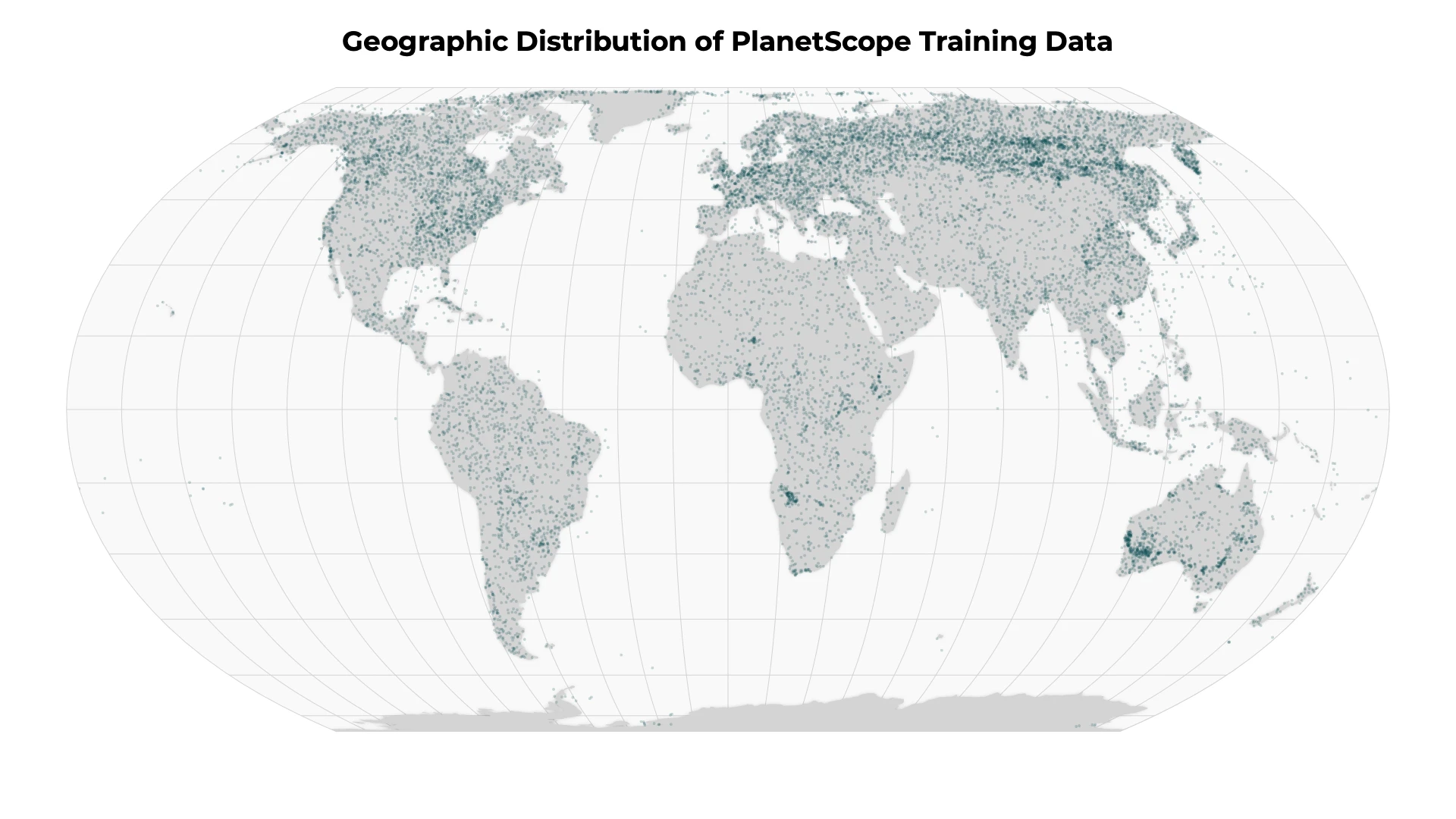
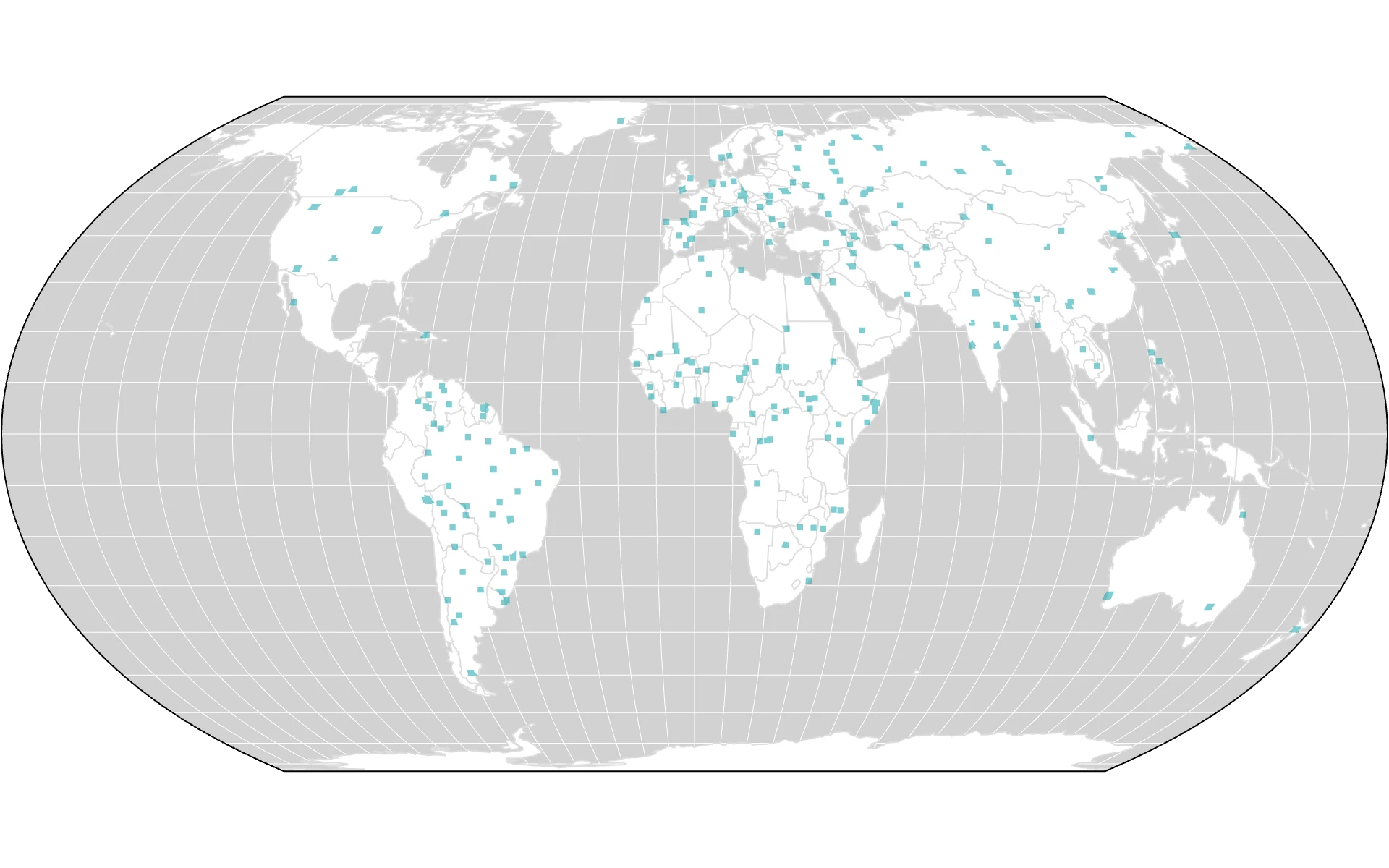
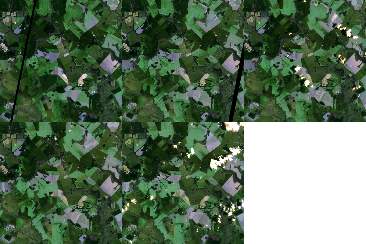
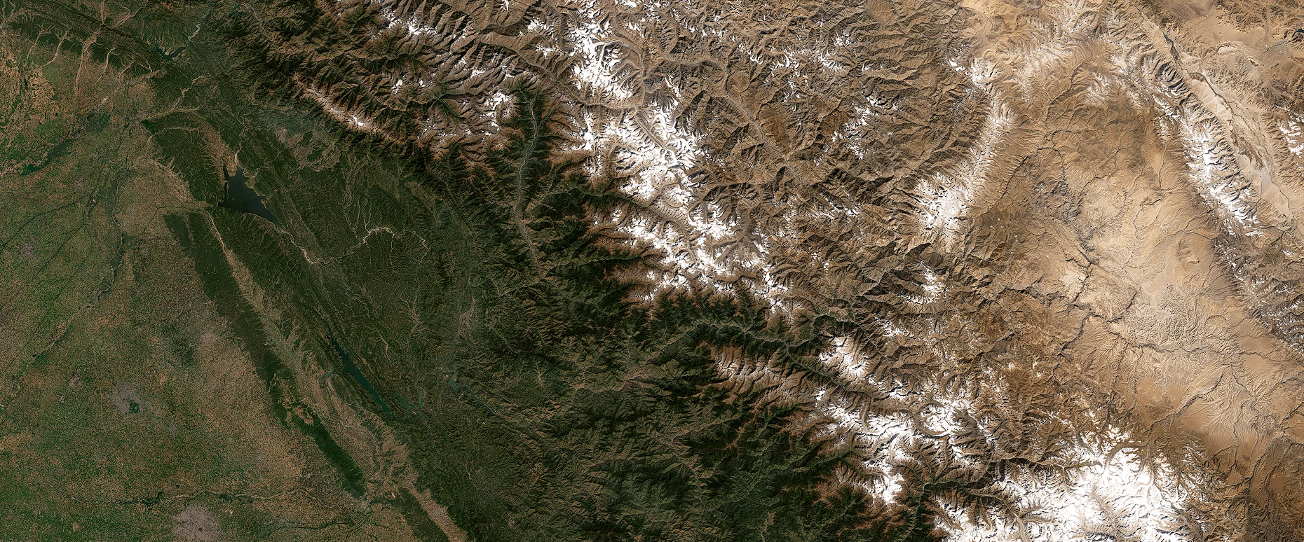
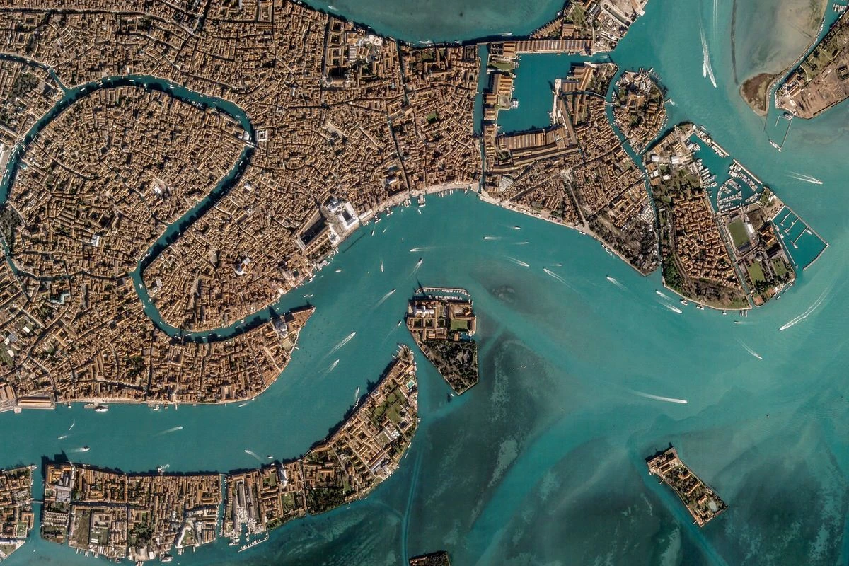
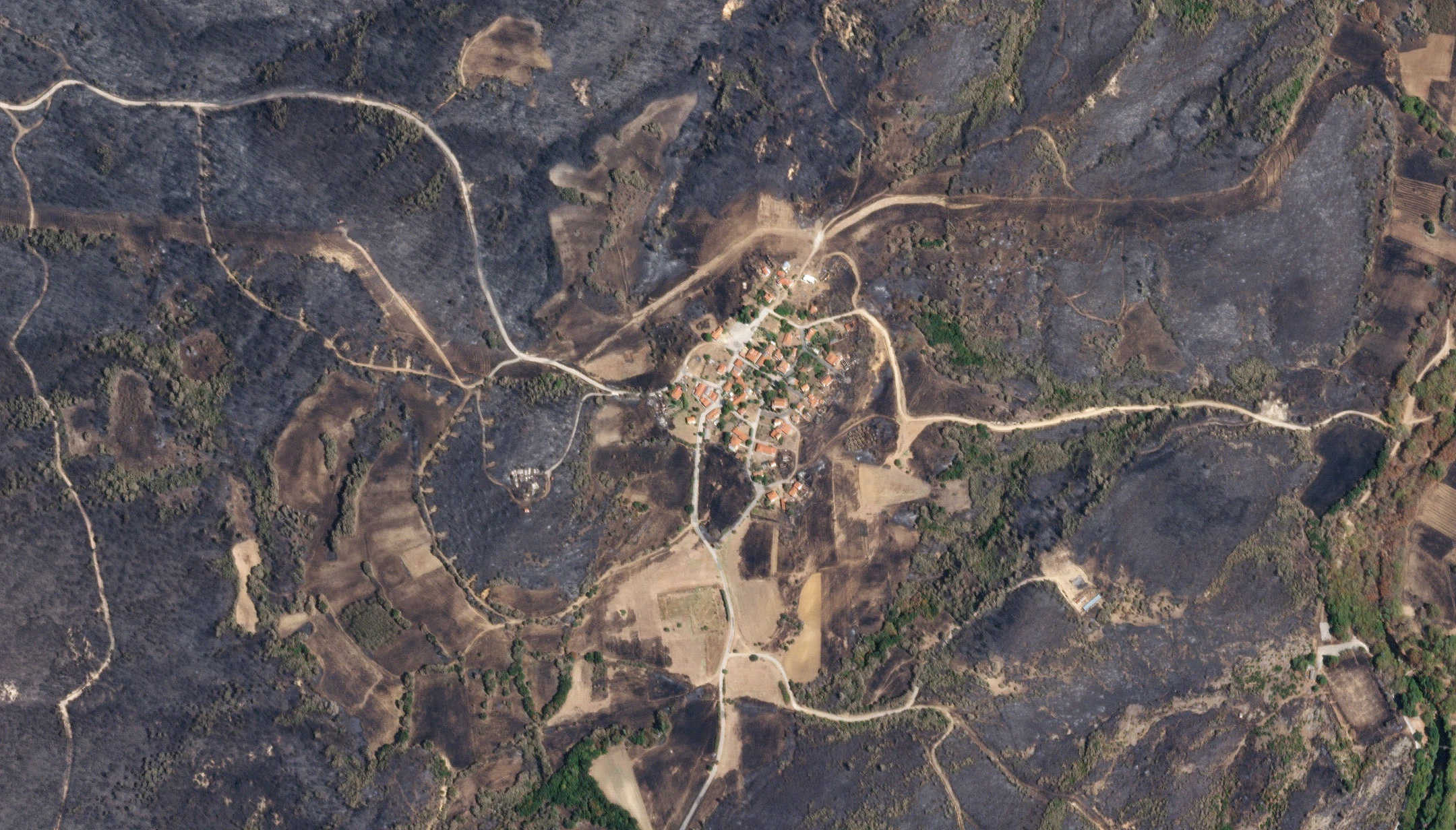
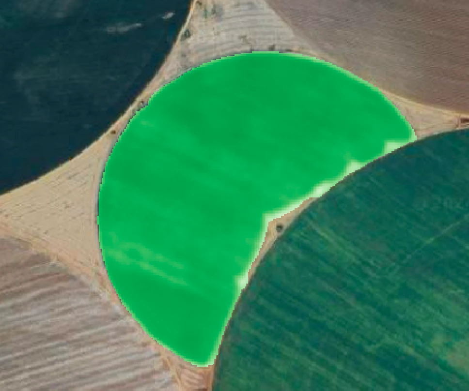
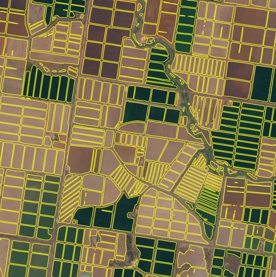





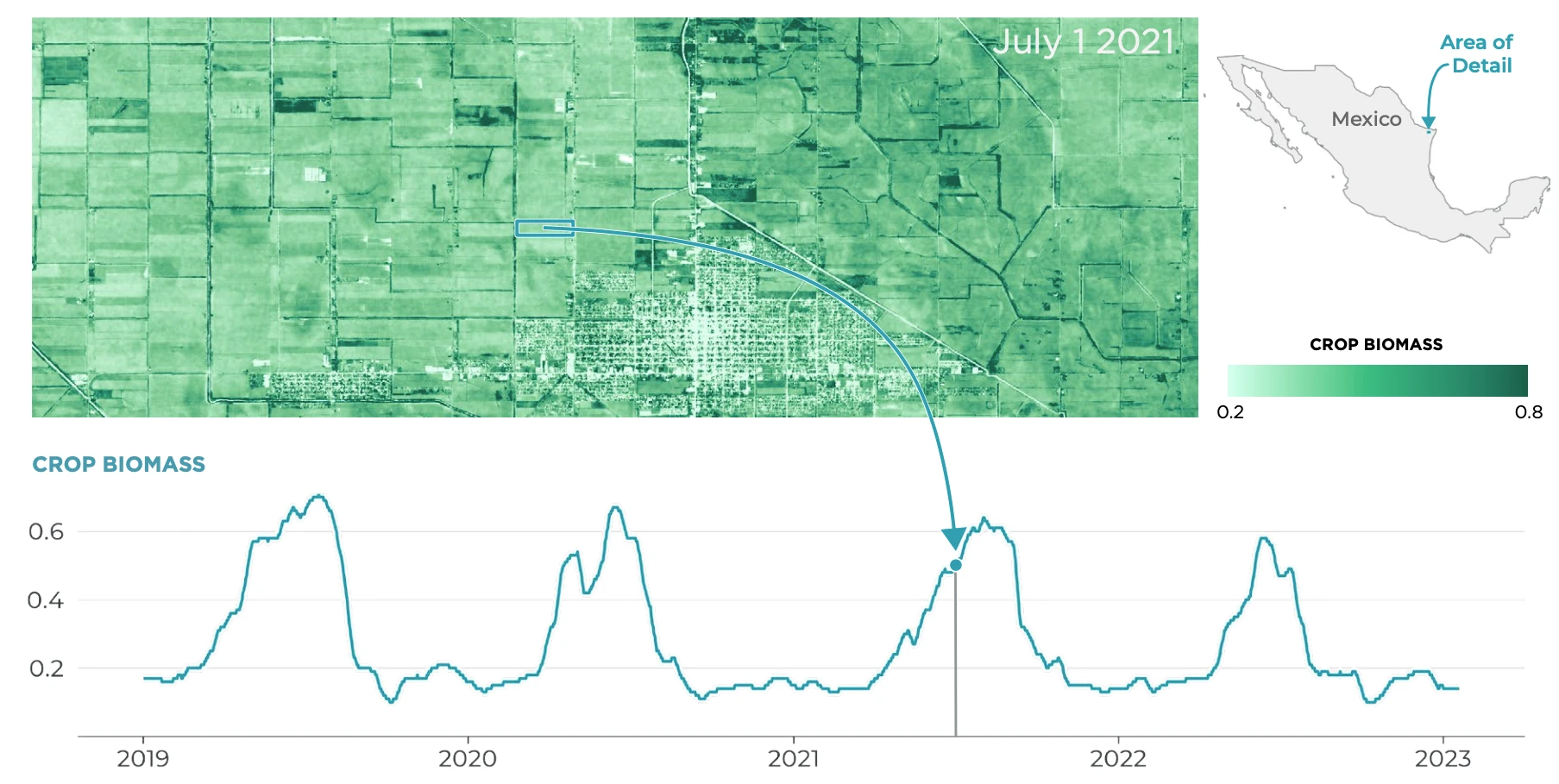
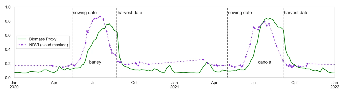


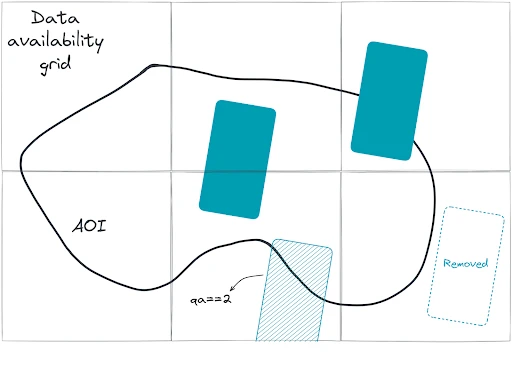
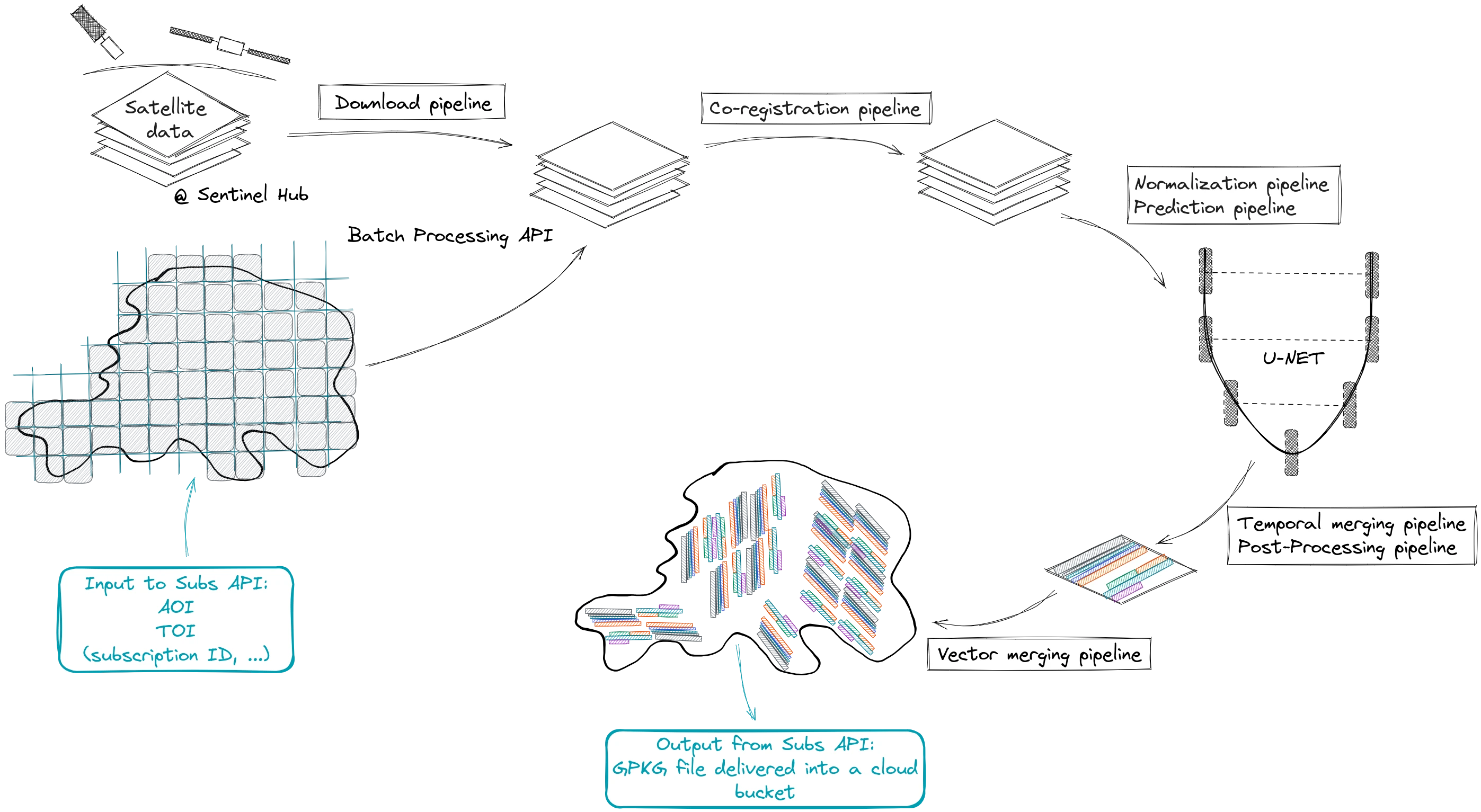
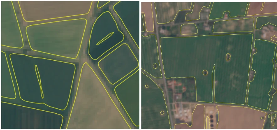

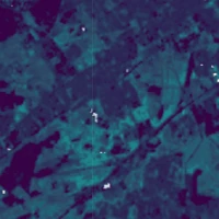
599km² [Visualize in the Browser →](https://insights.planet.com/analyze/browser/?zoom=12\&lat=44.7345\&lng=-0.676\&themeId=PLANET_SANDBOX\&visualizationUrl=https%3A%2F%2Fservices.sentinel-hub.com%2Fogc%2Fwms%2Ff006c031-60da-4262-bdf7-6fc4f1532d13\&datasetId=cc31cada-80d8-46fe-a746-43ac2f87b5da\&fromTime=2017-01-01T00%3A00%3A00.000Z\&toTime=2017-01-01T23%3A59%3A59.999Z\&layerId=ABOVEGROUND-CARBON-DENSITY\&demSource3D=%22MAPZEN%22) [![São Félix do Xingu, Brazil](/data/planetary-variables/forest_carbon_diligence/FCD_BRA.webp)](https://insights.planet.com/analyze/browser/?zoom=12\&lat=-6.7652\&lng=-52.3763\&themeId=PLANET_SANDBOX\&visualizationUrl=https%3A%2F%2Fservices.sentinel-hub.com%2Fogc%2Fwms%2Ff006c031-60da-4262-bdf7-6fc4f1532d13\&datasetId=e3d2a21c-cb75-4311-86ac-024385c85b9c\&fromTime=2017-01-01T00%3A00%3A00.000Z\&toTime=2017-01-01T23%3A59%3A59.999Z\&layerId=CANOPY-COVER\&demSource3D=%22MAPZEN%22) São Félix do Xingu, Brazil 2015-01-01 to 2017-01-01
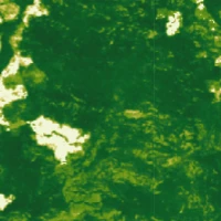
568km² [Visualize in the Browser →](https://insights.planet.com/analyze/browser/?zoom=12\&lat=-6.7652\&lng=-52.3763\&themeId=PLANET_SANDBOX\&visualizationUrl=https%3A%2F%2Fservices.sentinel-hub.com%2Fogc%2Fwms%2Ff006c031-60da-4262-bdf7-6fc4f1532d13\&datasetId=e3d2a21c-cb75-4311-86ac-024385c85b9c\&fromTime=2017-01-01T00%3A00%3A00.000Z\&toTime=2017-01-01T23%3A59%3A59.999Z\&layerId=CANOPY-COVER\&demSource3D=%22MAPZEN%22) [![Des Moines, USA](/data/planetary-variables/forest_carbon_diligence/FCD_USA.webp)](https://insights.planet.com/analyze/browser/?zoom=12\&lat=41.2969\&lng=-93.959\&themeId=PLANET_SANDBOX\&visualizationUrl=https%3A%2F%2Fservices.sentinel-hub.com%2Fogc%2Fwms%2Ff006c031-60da-4262-bdf7-6fc4f1532d13\&datasetId=f3312c82-edea-42a1-8c9d-ada86ddcc857\&fromTime=2016-01-01T00%3A00%3A00.000Z\&toTime=2016-01-01T23%3A59%3A59.999Z\&layerId=CANOPY-HEIGHT\&demSource3D=%22MAPZEN%22) Des Moines, USA 2015-01-01 to 2017-01-01

581km² [Visualize in the Browser →](https://insights.planet.com/analyze/browser/?zoom=12\&lat=41.2969\&lng=-93.959\&themeId=PLANET_SANDBOX\&visualizationUrl=https%3A%2F%2Fservices.sentinel-hub.com%2Fogc%2Fwms%2Ff006c031-60da-4262-bdf7-6fc4f1532d13\&datasetId=f3312c82-edea-42a1-8c9d-ada86ddcc857\&fromTime=2016-01-01T00%3A00%3A00.000Z\&toTime=2016-01-01T23%3A59%3A59.999Z\&layerId=CANOPY-HEIGHT\&demSource3D=%22MAPZEN%22) --- Copy for LLM[View as Markdown](https://docs.planet.com/data/planetary-variables/forest-carbon-diligence/techspec/) # Technical Specification ![Figure 1: Changes in total aboveground carbon stocks over a simulated forest carbon project boundary in Ucayali, Peru.](/data/planetary-variables/forest_carbon_diligence/forest-carbon-change-ucayali.webp) Figure 1: Changes in total aboveground carbon stocks over a simulated forest carbon project boundary in Ucayali, Peru. This document describes the Planet Forest Carbon Diligence product. It is intended for users of geospatial data interested in working with Forest Carbon Diligence, which estimates aboveground carbon density, canopy height, and canopy cover. Planet’s Forest Carbon Diligence products quantify—globally and annually—how much carbon is stored in trees, the area occupied by trees, and how tall they are. This is done using cutting edge machine learning models that fuse a rich archive of historical satellite observations with high quality, laser-derived reference data. Modeling benchmarks include an extensive archive of high resolution airborne LiDAR data for training and evaluating the height and cover models, and a global carbon dataset derived from two spaceborne LiDAR missions. This novel approach builds on decades of open data and open science, and was designed to maximize accuracy, transparency, and trust based on well-known standards. Mapping and monitoring forest carbon dynamics comes with uncertainty. Forest Carbon Diligence embraces uncertainty by reporting multiple pixel-level uncertainty metrics, including observation quality scores and prediction intervals for each dataset, each designed to support uncertainty propagation into user workflows. Jurisdictional and voluntary carbon monitoring programs require high quality, accessible, and globally consistent data on the state of the world’s forests, and how they are changing. The Forest Carbon Diligence products were designed to support these needs. Planet is committed to transparency and open science, and has published a full methods and validation report describing this product ([Anderson et al., 2025](https://doi.org/10.32942/X2KW7H)). **The features of Planet’s Forest Carbon Diligence data:** * A multi-year, GEDI-like forest carbon data product with wall-to-wall spatial coverage. * 12-year series quantifying annual patterns of aboveground carbon density, canopy cover and canopy height. * Full global coverage of the terrestrial biosphere at 30m resolution. * All models calibrated and evaluated with high quality reference data. * \>2 million km2 of airborne LiDAR used to train canopy cover and canopy height models. * \>80 million spaceborne LiDAR (GEDI, ICESat-2) samples used to train aboveground carbon model. * Novel cloud masking, pixel selection, multi-sensor fusion, and temporal harmonization techniques developed to minimize year-over-year measurement variability. * Calibrated, pixel-level prediction intervals support uncertainty propagation to downstream analyses. * Day-of-measurement and satellite data quality scores provide insights into prediction timing and quality. * GEDI-based model calibration enables independent validation of our product and simplifies intercomparison with a well-known global standard. ## Product Specifications Table 1: Forest Carbon Diligence product specification | Specification | Value | | ------------------- | ------------------------------------------------------- | | Metrics | Canopy cover, canopy height, aboveground carbon density | | Spatial extent | Global land mass > -60S and < 75N, excluding ice sheets | | Spatial resolution | 0.00025° (± 30 x 30 m) | | Temporal extent | 2013 - Present. | | Temporal resolution | Annual | | Temporal period | Jan 01 - Dec 31. | Canopy cover quantifies the percentage of area occupied by trees within a pixel, where a tree is defined as vegetation 5 meters or taller. This metric will be most sensitive to tree clearing events like timber harvest or deforestation, but is also sensitive to seasonal leaf-on variation and to drought. Canopy height quantifies the average stand height of trees within each pixel. Because this is a spatial average over a moderate resolution, the modeled height values are shorter than the tallest individual tree within a pixel. Aboveground carbon density quantifies the expected density of carbon stored in woody biomass across the landscape, measured in mass per area (megagrams of carbon per hectare). It is not a direct estimate of the total carbon in that pixel, as the spatial resolution of each pixel is less than one hectare. To estimate total carbon in a pixel, users should normalize these values to account for the size of each pixel, or average the density values to 1 hectare in an equal area projection. ## Asset Properties This tables specifies the properties of the data assets delivered by the [Planet Subscriptions API](https://docs.planet.com/develop/apis/subscriptions.md). Table 2: Forest Carbon Diligence data resource properties | Metric | Asset Name | Units | Type | Typical Range | No Data Value | Band Count | | -------------------------- | ---------- | ----- | ----- | ------------- | ------------- | ---------- | | Canopy Cover | cc | % | UINT8 | 0 - 100 | 255 | 1 | | Canopy Height | ch | m | UINT8 | 0 - 50 | 255 | 1 | | Aboveground Carbon Density | acd | Mg/ha | INT16 | 0 - 300 | 32767 | 1 | | CC Uncertainty | cc-uc | % | UINT8 | 0 - 100 | 255 | 2 | | CH Uncertainty | ch-uc | m | UINT8 | 0 - 80 | 255 | 2 | | ACD Uncertainty | acd-uc | Mg/ha | INT16 | 0 - 400 | 32767 | 2 | | CC Change Detection | cc-change | n/a | UINT8 | 0 - 2 | 255 | 1 | | CH Change Detection | ch-change | n/a | UINT8 | 0 - 2 | 255 | 1 | | Quality Flags | acd-qa | n/a | UINT8 | 0 - 224 | 255 | 1 | | Day of Year | acd-doy | day | INT16 | 0 - 366 | 32767 | 1 | The `cc`, `ch`, and `acd` assets contain the predicted values of canopy cover, canopy height, and aboveground carbon density in their natural units. Quality flag and day of year data are provided for all metrics (for example, `cc-qa`, `ch-qa`, `acd-qa`). They are only listed once in the table because they contain duplicate information across metrics. ### Uncertainty Bounds Table 3. Uncertainty band descriptions | Uncertainty Band | Description | | ---------------- | ---------------------------------------- | | Q05 (band 1) | Lower prediction bound (5th percentile) | | Q95 (band 2) | Upper prediction bound (95th percentile) | Uncertainty data are provided as calibrated 90% prediction intervals for each pixel in each year. These values are provided in the same units as their respective reference data. In other words, the pixel values and units are consistent between ACD and ACD-UC, between CC and CC-UC, and between CH and CH-UC. ### Change Assets Table 4. Change detection asset pixel values | Pixel Value | Description | | ----------- | -------------------------------------------------------------------- | | 0 | No change observed | | 1 | Fast change observed, such as deforestation or wildfire disturbance | | 2 | Slow change observed, such as reforestation or natural forest growth | The cc-change and ch-change assets classify annual changes that occur. These are the product of a time series model, which estimates whether a pixel experiences no change, fast change, or slow change from year to year. ### Quality Flags Table 5. QA pixel values | Pixel Value | Description | | ----------- | ----------------------------------------------------------------------------------------------------------------------------------------------------------------------------------------------------------------------------------------------------------------------------------------- | | 0-100 | Estimated observation quality. Low values indicate low quality observations, like hazy, cloudy, or off-season measurements. High values indicate high quality observations, like clear, cloud-free measurements captured during peak greenness. | | 213-214 | Year of closest available measurement. Some parts of the world experience persistent cloud cover or haze year-round, resulting in 0 valid measurements in a year. In these cases, the nearest-in- time clear observation is used. For example, 213 refers to 2013, and 222 refers to 2022 | Planet provides pixel-level QA data to indicate the relative quality of each pixel’s satellite data observation. These values are provided to diagnose whether observed changes might be the result of low quality measurements. ### Day of Year Table 6. DOY pixel values | Pixel Value | Description | | ----------- | ------------------------------------------------------------------------------------------------------------------------------------------------------------------- | | 0 | No measurement available. These primarily occur over water bodies where data are not provided. | | 1-366 | Julian day of the measurement. If this pixel has been filled with a nearest-in-time observation from a nearby year, the day of that year’s observation is reported. | Day of year pixel values encode the calendar day of the satellite observation. Since the number and quality of observations vary with the number of cloud-free observations, differences in observation dates between adjacent pixels can be large. This information can indicate seasonal differences between observations. It can also indicate whether an observation occurred prior to or following a disturbance. ## Input Data ![Figure 2: Extent and count of the airborne LiDAR data used for model training and evaluation.](/data/planetary-variables/forest_carbon_diligence/lidar-collection-training.webp) Figure 2: Extent and count of the airborne LiDAR data used for model training and evaluation. The Forest Carbon Diligence product uses multi-source, multi-scale earth observations data from a series of publicly available resources and derivative data products. The metrics derived from airborne and spaceborne LiDAR were treated as response variables, which were modeled using optical, radar, and derived feature data. Table 7: List of inputs for Forest Carbon Diligence production | Product | Description | | ----------------------------- | ------------------------------------------------------------------------------------------------------------------------------------------------------------------------------------------------------------------------------------------------------------------------------------------------- | | Airborne LiDAR | Point cloud data processed to canopy height and canopy cover rasters at 1m resolution then resampled to 30m resolution for model training | | Spaceborne LiDAR | [GEDI L4A](https://doi.org/10.3334/ORNLDAAC/1907) and [ICESat-2 ATLAS](https://doi.org/10.5067/D2E2L5GK7ER3) encode modeled estimates of aboveground biomass density. GEDI provides coverage over mid latitudes (<51.6 N, >51.6 S) and ICESat-2 provides coverage for high latitudes (>44.4 N) | | Surface Reflectance | The full scene archive of Landsat-8, Landsat-9, and Sentinel-2 were processed to BRDF-adjusted surface reflectance using FORCE ([Frantz 2019](http://doi.org/10.3390/rs11091124)). These scenes were masked for clouds, shadows, and haze and composited into annual best-available-pixel mosaics | | L-band RaDAR backscatter | L-band SAR mosaics from [ALOS PALSAR-2](https://www.eorc.jaxa.jp/ALOS/en/dataset/fnf_e.htm). Both HH and HV polarizations were downloaded for each year. No rescaling or normalization was applied to these data | | Wood density | Wood density estimates were used as features in the canopy height and canopy cover models. These estimates encode coarse scale (\~1 km) biogeographic information that might inform the mapping from remote sensing data to forest structural traits | | Digital Elevation Model (DEM) | Copernicus [GLO-30](https://doi.org/10.5270/ESA-c5d3d65) DEM are used for most of the global landmass, ALOS [AW3D30](https://www.eorc.jaxa.jp/ALOS/en/dataset/aw3d30/aw3d30_e.htm) is used where GLO-30 does not provide data | ## Methods ![Figure 3: Workflow diagram for Forest Carbon Diligence illustrating the flow of data for delivery.](/data/planetary-variables/forest_carbon_diligence/diligence-overview-diagram.webp) Figure 3: Workflow diagram for Forest Carbon Diligence illustrating the flow of data for delivery. The Forest Carbon Diligence products were created using multi-scale, publicly available EO data. These datasets were modeled in a stepwise process to balance the strengths and limitations of each dataset. Fully detailed methods, validation results, and data sources are described in [Anderson et al., 2025](https://doi.org/10.32942/X2KW7H). ### Airborne LiDAR Data Point cloud data were downloaded from a series of open data platforms, reprojected to a consistent coordinate system (EPSG:6933) and normalized in the Z dimension to height above ground. Ground point classifications provided in the source data were used for normalization. Buildings, bridges, noise, and other non-vegetation classes were removed from processing using the point classifications provided in the source data, when present. For datasets with no prior classifications, custom building and noise classifiers were used. Canopy height and canopy cover were rasterized from the normalized point cloud data at 1 m native resolution. Overall, 2,234,400 km2 of LiDAR data were processed and extracted for model training and evaluation (Fig. 2). Canopy height (m) was calculated as the tallest point within each grid cell using a modified pit-free canopy height model algorithm ([Khosravipour et al. 2014](https://doi.org/10.14358/PERS.80.9.863)). This is not restricted to trees as there is no height or size threshold for inclusion; the height of the tallest vegetation at each cell is recorded, be it grass, shrub, or tree. Canopy cover (%), also referred to as canopy density, is calculated as the number of LiDAR returns 5m and above divided by the total number of returns within each grid cell. This threshold tracks overstory vegetation cover, and can be interpreted as a proxy for canopy closure; cover increases in proportion to overstory foliage volumes. It can be interpreted as the complement to canopy gap fraction (CC = 1 − GF; [Coomes et al. 2017](http://dx.doi.org/10.1016/j.rse.2017.03.017)). Average resampling to a lower resolution reduces the range of observed canopy height values to approximately 0-40 m. Average resampling was selected because this implicitly weights pixel-level tree height measurements by crown diameter, and the combination of these variables is correlated with aboveground biomass across ecosystems ([Jucker et al. 2018](https://doi.org/10.1111/gcb.13388)). ### Spaceborne LiDAR Data AGBD estimates from GEDI v2.1 ([Dubayah et al. 2022](https://doi.org/10.3334/ORNLDAAC/2056)) and ICESat-2 ATLAS ([Montesano et al. 2024](https://doi.org/10.5067/D2E2L5GK7ER3)) were downloaded, merged, and organized into a harmonized dataset using a global equal area tile grid (see Gridding and Sampling). These two sources of AGBD estimates are complementary, with overlap, as GEDI provides coverage over mid latitudes (<51.6 N, >51.6 S) and ICESat-2 provides coverage for high latitudes (>44.4 N). A series of quality filters were applied to the GEDI observations, selecting samples from power beams, collected at night, excluding steep slopes, and excluding orbits with high geolocation error. ICESat-2 data were filtered by the data providers. Additional outlier detection was applied to both GEDI and ICESat-2 observations, which identified and removed anomalously tall RH98 observations, particularly over sparsely arbored areas. Overall, 586 million GEDI observations and 15 million ICESat-2 observations were retained after filtering (30% and 99% of the original observations, respectively). A final spatially balanced random sampling step yielded 81.6 million waveforms to be used for training and evaluation, reducing bias in oversampled regions and better approximating a geographically uniform random sample ([Meyer and Pebesma 2022](https://doi.org/10.1038/s41467-022-29838-9)). ### Surface Reflectance Multispectral surface reflectance data provided 6 of the 9 feature bands used for the forest structure models. Surface reflectance is sensitive to patterns of vegetation growth and structure, with optical variation driven by a combination of leaf-level and canopy-level growth and structure metrics ([Jordan 1969](https://doi.org/10.2307/1936256), [Knipling 1970](https://doi.org/10.1016/S0034-4257\(70\)80021-9), [Asner 1998](https://doi.org/10.1016/s0034-4257\(98\)00014-5), [Dalagnol et al. 2023](https://doi.org/10.5194/essd-15-345-2023)). The full scene archives of Landsat-8, Landsat-9, Sentinel-2A and Sentinel-2B were downloaded from public cloud storage. Each scene was processed to nadir BRDF-adjusted surface reflectance using the FORCE atmospheric correction and normalization algorithm ([Frantz 2019](https://doi.org/10.3390/rs11091124)). FORCE produces a scene-level QA mask classifying cloud, shadow, haze, water, and snow using a modified version of FMask ([Qiu et al. 2019](https://doi.org/10.1016/j.rse.2022.113375), [Skakun et al. 2022](https://doi.org/10.1016/j.rse.2022.112990)). Sentinel-2 scenes were average resampled to match Landsat’s resolution. To reduce false negative cloud detections, a custom cloud and shadow mask was applied to update each scene’s QA mask. Only the six bands shared across instruments were retained: \[B, G, R, NIR, SWIR-1, SWIR-2]. Annual surface reflectance mosaics were created beginning in 2013, which marks the launch of Landsat-8 ([Roy et al. 2014](https://doi.org/10.1016/j.rse.2014.02.001)). These mosaics were created using a custom best-available-pixel compositing method, adapted from White et al. 2014. Best-pixel methods show strong temporal consistency compared to percentile-based composites, though this may come at the expense of radiometric uniformity ([Matasci et al. 2018](https://doi.org/10.1016/j.rse.2018.07.024)). The following quality metrics were used: * **Haze score**. Aerosol optical depth (AOD) estimates from FORCE were used to indicate haze. Quality scores were set inversely proportional to AOD scores, where lower AOD indicates a higher quality score. * Distance to cloud score. Some cloud edges are not correctly classified by the strict cloud mask, so the euclidean distance to each cloudy pixel downranked pixels close to cloud detections. * **Solar zenith angle score**. Sun-sensor geometry is the primary driver of variation in surface reflectance, leading to large differences in observation conditions over the year, especially at high or low latitudes. Solar zenith angle was used as a quality metric to prioritize scenes collected during well-lit observation conditions, which improves retrieval of vegetation structural information ([Dalagnol et al. 2023](https://doi.org/10.5194/essd-15-345-2023)). * **Day of year score**. Because vegetation varies throughout the year in response to seasonal change, a day of year score was defined to prioritize spring measurements. * **Sensor score**. Landsat scenes were ranked lower than Sentinel-2 scenes because the Sentinel-2 cloud mask reports higher precision scores and includes fewer false negatives ([Frantz et al. 2018](https://doi.org/10.1016/j.rse.2018.04.046)). The pixel composite method addressed three needs. First was to maximize consistency in the observation conditions for each pixel. The compositor included scoring factors based on sun angle, expected time of peak greenness, distance to clouds, aerosol density, and instrument type. Pixel quality increased as solar elevation increased, at times closest to peak greenness, as aerosol content decreased, and for Sentinel-2 observations over Landsat-8/9 observations. The second goal of the compositor was to provide a quantitative flag for observation quality. Pixel quality scores provide information regarding the expected reliability of each observation, allowing users to filter or weight observations based on pixel quality. Finally, the compositor records the Julian day of the best pixel, providing a timestamp for when each observation occurred. ### L-Band RaDAR, Wood Density, and Elevation Data Annual, radiometrically balanced L-band Synthetic Aperture Radar mosaics from ALOS-PALSAR-2 were downloaded from JAXA’s HTTP server. The HH and HV polarizations comprise 2 of the 9 total predictor bands used for the canopy cover and canopy height models. Active microwave measurements are directly sensitive to aboveground plant water content, and L-Band measurements in particular are typically sensitive to the water content of large, woody biomass components, like tree trunks and branches, indirectly measuring key components of stand-level vegetation structure ([Shimada et al. 2011](https://doi.org/10.1109/JSTARS.2010.2077619), [Konings et al. 2019](http://dx.doi.org/10.1111/nph.15808)). The HH/HV polarization data were not transformed, save for data type and nodata value harmonization across datasets. Global estimates of wood density were generated at a 1 km resolution via gradient boosted regression of field-observed wood density against principal-component normalized WorldClim and Soilgrids data. This is the final predictor used for the canopy cover and canopy height models, and was included as an index of plant community biogeography to identify non-stationary relationships between target and predictor variables by vegetation type ([Hawkins 2011](https://doi.org/10.1111/j.1365-2699.2011.02637.x)). In total 396,694 field inventory plots were used for training, including data from national forest inventories, ecological monitoring networks, research consortiums, and open data repositories. Elevation data were used as a predictor for the aboveground carbon density model. This allowed the model to learn nonstationary carbon-topography relationships at local and regional scales, capturing fine-scale topoedaphic drivers of carbon storage in slopes and floodplains ([Marvin et al. 2014](https://doi.org/10.1073/pnas.1412999111), [Taylor et al. 2015](https://doi.org/10.1371/journal.pone.0126748), [Jucker et al. 2018](https://doi.org/10.1111/ele.12964)) and along elevation gradients ([Asner et al. 2014](https://doi.org/10.5194/bg-11-843-2014), [Mahli et al. 2017](https://doi.org/10.1111/nph.14189), [Marifatul Haq et al. 2022](https://doi.org/10.1016/j.foreco.2022.120442)). Elevation data were primarily sourced from the Global 30 m Copernicus Digital Elevation Model ([ESA 2022](https://dataspace.copernicus.eu/explore-data/data-collections/copernicus-contributing-missions/collections-description/COP-DEM)). Since this dataset does not include data over Armenia and Azerbaijan, values for those countries were derived from the ALOS World-3D DEM ([Tadono et al. 2014](https://www.eorc.jaxa.jp/ALOS/en/dataset/aw3d30/aw3d30_e.htm)). ### Canopy Height and Canopy Cover Models Deep learning regression models were trained to predict mean canopy height and canopy cover independently at 30 m nominal resolution using surface reflectance, HH/VV backscatter, and wood density data as feature variables and airborne LiDAR as response variables. The feature and response variables were normalized to a common range using robust scaling. U-Net convolutional neural network architectures were selected for their robust performance in mapping ecological patterns from EO data ([Ronneberger et al. 2015](https://doi.org/10.1007/978-3-319-24574-4_28), [Broderick et al. 2019](https://doi.org/10.1016/j.tree.2019.03.006), [Kattenborn et al. 2021](https://doi.org/10.1016/j.isprsjprs.2020.12.010), [Wagner et al. 2024](https://doi.org/10.3390/rs12101544)). Training data were generated by randomly sampling 128x128 pixel tiles from regions with coincident airborne LiDAR data. The year of the satellite data closest to the LiDAR acquisition was used for temporal matching. A total of 1,099,559 samples were extracted at an average sample density of 2 points per square kilometer using uniform random geographic sampling. Samples were randomly assigned to training/validation sets (67%) or interval calibration/testing (33%) sets. The training/validation data were then randomly split 70/30, and the interval calibration/testing data were randomly split 20/80. Training data were used to fit model parameters. Validation data were used to approximate out of sample predictive performance during training. Interval calibration data were used in conformal inference to generate 90% prediction intervals. Test data were used to evaluate predictive performance. ### Time Series Model ![Figure 4: Statistical model for estimating canopy height and canopy cover over time. (A) A time series is generated from the raw predictions for times t=1, … T. (B) Three models are fit for each pixel: a constant model to represent the mean (blue), a changepoint model to represent sudden change (red), and a spline model to represent gradual change (orange). (C) The preferred model for each pixel is used to generate expected values (green) and standard errors (blue) for each time step.](/data/planetary-variables/forest_carbon_diligence/fcd_denoising_conceptual.webp) Figure 4: Statistical model for estimating canopy height and canopy cover over time. (A) A time series is generated from the raw predictions for times t=1, … T. (B) Three models are fit for each pixel: a constant model to represent the mean (blue), a changepoint model to represent sudden change (red), and a spline model to represent gradual change (orange). (C) The preferred model for each pixel is used to generate expected values (green) and standard errors (blue) for each time step. The Diligence U-net models predict height and cover independently for each year, and these predictions contain non-structural variation related to phenology, illumination, and sensor calibration. This residual prediction variation was minimized using statistical models. For each pixel, three models were fit (Fig. 4): * A constant-in-time model, which represents stability over time * A spline model, which represents gradual change * A changepoint model, which represents fast change The constant model assumes that all variation in predictions is due to noise, and assumes height or cover remains stable over time or when changes are minimal relative to prediction noise (for example, slow growth that is not detectable). The spline and changepoint models capture slow and fast changes, respectively. Regularized B-splines are used to estimate non-linear trends, while the changepoint model included an additional discrete change point parameter at the timestep with the greatest change in predicted height or cover. The preferred model for each pixel was selected using Akaike's Information Criteria (AIC). An additional heuristic was applied to reduce noise: if the coefficient of variation (CV) over time for the selected model's predictions is below a threshold, the constant-in-time model was selected. This CV threshold is a hyperparameter tuned alongside the AIC threshold. Once a preferred model was selected for each pixel, predictions were generated and the standard errors were used to quantify pixel-level uncertainty for height and cover. Time series outputs for each year are provided as an additional data asset, with categorical classes mapping no change, fast change, and gradual change (classes \[0, 1, 2], respectively). ### Canopy Height and Canopy Cover Uncertainty Standard errors from the height and cover time series models were used to construct 90% prediction intervals: $[y_{pred} - \widehat{q} \cdot \sigma_{pred}, y_{pred} + \widehat{q} \cdot \sigma_{pred}]$ where $y_{pred}$ is a predicted value from the time series model, $\sigma_{pred}$ is the standard error of the prediction, and $\widehat{q}$ is a parameter estimated using withheld data via split conformal inference. Split conformal inference uses disjoint partitions of a dataset to produce well-calibrated prediction intervals. These are 90% prediction intervals that contain the true value approximately 90% of the time ([Angelopolous and Bates 2021](https://doi.org/10.48550/arXiv.2107.07511)). A calibration dataset is used to estimate $\widehat{q}$, a scalar quantity that determines the width of the interval relative to the standard error to achieve 90% coverage. After generating predictions with $\widehat{q}$, empirical interval coverage is quantified on a spatially non-overlapping test set. Test set coverage was 90.0% for canopy cover and 90.1% for canopy height. ### Aboveground Carbon Density Model Light gradient-boosting machine (LightGBM) regression models were trained to predict GEDI L4A and ICESat-2 aboveground biomass as a function of predicted mean canopy height, canopy cover, elevation, and location. Location data were encoded using SatCLIP positional embeddings ([Klemmer et al. 2023](https://doi.org/10.48550/arXiv.2311.17179)). The relationships between forest structure and aboveground biomass vary across plant communities, biomes, and topographic gradients, and these shifting relationships are explicitly encoded in the GEDI L4A biomass algorithm ([Jucker et al. 2018](https://doi.org/10.1111/gcb.13388), [Duncanson et al. 2022](https://doi.org/10.1016/j.rse.2021.112845), [Kellner et al. 2023](https://doi.org/10.1029/2022EA002516), [Ma et al. 2023](https://doi.org/10.1038/s41477-023-01543-5)). Incorporating location features into a tree-based regression model can represent multiple nonstationary relationships: specifically, between predictors and both the mean biomass density and its associated uncertainty ([Hawkins, 2011](https://doi.org/10.1111/j.1365-2699.2011.02637.x)). 10-fold spatial cross validation was used to assess out-of-sample predictive performance, where each of the 7,408 tiles containing GEDI or ICESat-2 biomass estimates were assigned to one of ten partitions ([Meyer and Pebesma 2022](https://doi.org/10.1038/s41467-022-29838-9)). For each fold, 5% of the training data were randomly withheld for uncertainty calibration. Model hyperparameters were evaluated using Bayesian optimization of cross-validation RMSE on a random 25% of data. The number of trees, the leaves in each tree, as well as both L1 and L2 regularization were modified. Final hyperparameter selection was also informed by visual inspection of predictions and external intercomparisons. Uncertainty was quantified via conformalized quantile regression, which yielded 90% prediction intervals where interval widths vary nonlinearly as a function of model predictors ([Romano et al. 2019](https://doi.org/10.48550/arXiv.1905.03222)). In particular, LightGBM quantile regressors were fit to estimate the 5% and 95% quantiles, then conformalized to obtain prediction intervals with strong coverage guarantees on unseen data ([Angelopolous and Bates 2021](https://doi.org/10.48550/ARXIV.2107.07511)). Conformalized quantile regression was selected for two reasons. First, nonstationary errors were expected to vary nonlinearly as a function of model inputs, including location. Second, reported uncertainties for footprint-level biomass estimates generally underestimate on-orbit uncertainties that arise from error in relative height estimates (Duncanson et al. 2022). Prediction intervals from conformal inference, in contrast, reflect the empirical distribution of on-orbit data, propagating both measurement- and model-based uncertainty. Finally, aboveground biomass density is converted to aboveground carbon density by multiplying by the global mean carbon concentration: 0.476 ([Martin et al. 2018](https://doi.org/10.1038/s41561-018-0246-x)). ### Post Processing Estimates of height, cover, and aboveground carbon density were minimally post-processed using simple heuristics. To reduce low noise, canopy cover values < 5% were set to zero. If canopy cover was zero at both the beginning and the end of the time series, then all annual cover values were set to zero. Where canopy cover was estimated as zero, canopy height and aboveground carbon density were also set to zero. ## Data Quality ![Figure 5: Model performance evaluated on withheld samples (n=360,853 tiles) for (A) mean canopy height and (B) canopy cover at 30 m resolution. Performance metrics were computed using the full withheld datasets but the plots were subset to 1 million random samples for visualization. (C) Aboveground biomass model performance evaluated against GEDI L4B data at 1 km resolution. A minimum of 20 points per grid cell were used for visualization.](/data/planetary-variables/forest_carbon_diligence/model-performance-scatter-plots.webp) Figure 5: Model performance evaluated on withheld samples (n=360,853 tiles) for (A) mean canopy height and (B) canopy cover at 30 m resolution. Performance metrics were computed using the full withheld datasets but the plots were subset to 1 million random samples for visualization. (C) Aboveground biomass model performance evaluated against GEDI L4B data at 1 km resolution. A minimum of 20 points per grid cell were used for visualization. The evaluation framework for this product includes two primary components: withheld data evaluation, and intercomparison. Withheld data evaluation refers to comparisons with samples of directly comparable observations, like airborne or spaceborne LiDAR data. Intercomparison evaluates modeled Diligence estimates against modeled estimates from external sources, like field plots and third party satellite observations. This distinction is particularly important when comparing carbon density or biomass density data. To fully evaluate the quality of this product, we hihgly recommend reading the full methods and validation report describing this product ([Anderson et al., 2025](https://doi.org/10.32942/X2KW7H)). ### Airborne LiDAR Comparison The canopy height model has a root mean squared error (RMSE) of $2.9\ m$, mean absolute error (MAE) of $1.5\ m$, bias of $0.04\ m$, and an $r^2$ value of $0.83$ (Fig. 5A). The canopy cover model has $RMSE = 14.3%$, $MAE = 8.25%$, $bias = 0.4%$, and $r^2 = 0.79$ (Fig. 5B). ### GEDI L4A and ICESat-2 Comparison Based on 10-fold geographic cross validation, the aboveground biomass model has a mean RMSE of $55.27\ Mg \cdot ha^{-1}\ (sd = 2.18)$, mean MAE of $24.2\ Mg \cdot ha^{-1}\ (sd = 0.87)$, mean bias of $-0.06\ (sd = 0.39)$, and a mean $r^2$ value of $0.638\ (sd = 0.01)$. Uncertainty estimation showed empirical interval coverage on withheld data was 92.07%, and the mean interval width is $100.9\ Mg \cdot ha^{-1}$. ### GEDI L4B Comparison Comparing mean aboveground biomass density at a 1 km scale against GEDI L4B — a product that statistically aggregates L4A footprints and is not independent from the training data — reports model performance scores of $RMSE = 30.77\ Mg \cdot ha^{-1}$, $MAE = 13.49 Mg \cdot ha^{-1}$, $bias = -5.0 Mg \cdot ha^{-1}$, and $r^2 = 0.819$ (Fig. 5C). Further resampling to 1 degree grid cells shows strong agreement between Diligence and GEDI L4B ($r=0.98$, $bias=-5.0$, $RMSE=14.03$, $MAE=8.37$) but identifies particularly high disagreement in mountainous regions. These results demonstrate the benefits of spatial aggregation, reducing noise in both the model predictions and the L4A footprints. ## Known Limitations and Caveats **Unmasked clouds/shadows/haze** may occur in certain cases. Significant effort went into developing minimizing cloud and atmospheric contamination from surface reflectance data, but in some cases commission errors can still be an issue. This is most common over the Congo Basin, which experiences year-round cloudy and smoky conditions. **Circular spatial artifacts** in model predictions arise due to the pixel selection logic that downweights pixel quality scores by distance to cloud edges. This can lead to large temporal differences between adjacent pixels. Information on expected pixel quality and the day of observation are encoded in the QA and DOY products, which can be used to filter out low quality observations from a change analysis. **Square spatial artifacts** are the result of the tile-based U-Net architecture, and are most prominent over heavily forested areas in the canopy height predictions. These artifacts are often predicted to be 1-2m taller than surrounding pixels, and are typically well within the uncertainty bounds, but are visually distinctive. Downsampling typically minimizes this effect. **Occasional over-prediction over the built environment** due to high rates of double-bounce radar backscattering among buildings. Interpret values over urban areas with caution. **Prediction intervals can be asymmetric**. For example, since carbon model predictions typically underestimate stocks, upper prediction intervals (p95) are often wider than the lower prediction interval (p05). On average, the prediction intervals will contain the true pixel value with probability of 0.9. ## Coverage Map ![Figure 7. Data availability map for the forest carbon diligence product. Land above 75 North or below 60 South are excluded. Some small islands were excluded](/data/planetary-variables/forest_carbon_diligence/fcd-global-coverage.webp) Figure 7. Data availability map for the forest carbon diligence product. Land above 75 North or below 60 South are excluded. Some small islands were excluded --- Copy for LLM[View as Markdown](https://docs.planet.com/data/planetary-variables/forest-carbon-diligence/validation/) # Validation Report This document provides validation and intercomparison results for the Planet Forest Carbon Diligence products. It is intended for users of geospatial data interested in working with Forest Carbon Diligence data, which estimates aboveground carbon density, canopy cover, and canopy height. The Forest Carbon Diligence products quantify — globally and annually — the density of carbon stored in trees, the area occupied by trees, and stand-level mean canopy height. These estimates are produced from machine learning models trained on historical satellite observations, airborne LiDAR data, and spaceborne LiDAR data. See the [Forest Carbon Diligence Technical Specification](https://docs.planet.com/data/planetary-variables/forest-carbon-diligence/techspec.md) for more information about methods. [Download Planet Forest Carbon Diligence Validation Report →](https://planet.widen.net/s/d669jncqld/planet-userdocumentation-forestcarbonvalidation) --- Copy for LLM[View as Markdown](https://docs.planet.com/data/planetary-variables/forest-carbon-monitoring/) # Forest Carbon Monitoring ![Header Thumbnail](/data/planetary-variables/forest_carbon_monitoring/zimbabwe_docs.webp) The Forest Carbon Monitoring product is composed of a bundle of data resources: Canopy Height, Canopy Cover, and Aboveground Live Carbon at 3-meter spatial resolution. These data resources are produced quarterly over the entire landmass of the Earth (between 75° N and 60° S). The archive currently extends back to 2021. See the Technical Specification for more details. ## Basic Facts | **Property** | **Info** | | ---------------------- | ------------------------------------------------------------------------------------------------------------------------------------------------------------------------------- | | Spatial resolution | 3 m | | Sensor/Input Data | Airborne LiDAR, LiDAR (GEDI), PlanetScope surface reflectance, Forest Carbon Diligence, Digital Elevation Model (DEM) | | Revisit time | Quarterly | | Spatial coverage | Global | | Data availability | Q1 2021 - present | | Available measurements | Canopy Height, Canopy Cover, and Aboveground Live Carbon | | Common usage/purpose | Planet's Forest Carbon Monitoring products provides timely, operational, near-tree-scale insights into global changes in canopy cover, canopy height, and above carbon density. | Forest Carbon Monitoring Data Releases New Forest Carbon Monitoring data are released quarterly (March, June, September, December) on the last day of the month. ## Use Cases **Reforestation Monitoring** - Forest Carbon Monitoring provides comprehensive data to identify and analyze reforestation and restoration projects. These efforts help trap carbon, support sustainable harvesting efforts, and may provide local economic benefits through tourism, public funding, or renewable resources. Stakeholders can use Forest Carbon to identify potential reforestation sites and monitor, analyze, and report on ongoing projects. **Degradation Monitoring** - Detect single tree selective harvest or other small disturbances with our 3m resolution product. Brings powerful monitoring capacity to REDD+ and improved forest management (IFM) based carbon projects. With updates every quarter, you and your stakeholders will no longer have to wait years to know if a project is on track. ## API Access Information | API | Available | Notes | | ----------------- | --------- | ----- | | Data API | ❌ | | | Orders API | ❌ | | | Subscriptions API | ✅ | | | Analytics API | ❌ | | | Basemaps API | ❌ | | ### Subscriptions Access #### Canopy Height 3m Loading... #### Canopy Cover 3m Loading... #### Aboveground Carbon Density 3m Loading... For each request you make using the Subscriptions API, you'll get a dataset that includes forest carbon estimations for the specified TOI and AOI. For more information on the Subscriptions API and code samples, see the [API documentation](https://docs.planet.com/develop/apis/subscriptions/sources.md#planetary-variable-and-analysis-ready-source-types). ### Subscriptions Time of Interest The table below provides an example of the temporal periods and the date tags associated with Forest Carbon Monitoring data. When creating a subscription, the 'start\_time' must be set to the date tag or earlier, while the 'end\_time' must be set to a date after the date tag. | **Season** | **Quarter** | **Start** | **End** | **Date Tag** | | ---------- | ----------- | ---------- | ---------- | -------------------- | | Winter | Q1 2024 | 2023-12-21 | 2024-03-20 | 2023-12-21T00:00:00Z | | Spring | Q2 2024 | 2024-03-21 | 2024-06-20 | 2024-03-21T00:00:00Z | | Summer | Q3 2024 | 2024-06-21 | 2024-09-20 | 2024-06-21T00:00:00Z | | Fall | Q4 2024 | 2024-09-21 | 2024-12-20 | 2024-09-21T00:00:00Z | ## Additional Resources [📖Technical Specification](https://docs.planet.com/data/planetary-variables/forest-carbon-monitoring/techspec.md) [Get the details in the Forest Carbon Monitoring Technical Specification](https://docs.planet.com/data/planetary-variables/forest-carbon-monitoring/techspec.md) [🎓Planet University](https://university.planet.com/intro-to-forest-carbon-diligence-and-monitoring) [Get Started with Planet’s Forest Carbon Planetary Variable product for: global tree height, canopy cover and carbon raster.](https://university.planet.com/intro-to-forest-carbon-diligence-and-monitoring) [📓Guides](https://docs.planet.com/guides.md) [Visit our Guides page to find a collection of Jupyter Notebooks for hands-on learning.](https://docs.planet.com/guides.md) [📚APIs](https://docs.planet.com/develop/apis/subscriptions.md) [Learn more about the Planet Subscriptions API to obtain Forest Carbon data.](https://docs.planet.com/develop/apis/subscriptions.md) --- Copy for LLM[View as Markdown](https://docs.planet.com/data/planetary-variables/forest-carbon-monitoring/products/) # Products Below you will find a list of Data Resources available for the Forest Carbon Monitoring product.Each Data Resource has a series of associated Data Assets. We are continuoulsy working to improve the product, and periodically release new versions. We provide access to older versions of our products, but only produce data using the latest version at new timesteps. We recommend using the latest product version and reviewing the [version history in the changelog](https://docs.planet.com/develop/changelog.md?tag=forestCarbonMonitoring) associated with each release. ## Canopy Height 3m Loading... ## Canopy Cover 3m Loading... ## Aboveground Carbon Density 3m Loading... --- Copy for LLM[View as Markdown](https://docs.planet.com/data/planetary-variables/forest-carbon-monitoring/sandbox/) # Forest Carbon Monitoring Sandbox Data This Planet Sandbox Data collection for Forest Carbon Monitoring provides sample data over specific areas and times of interest. The data is available to paid and trial accounts that include processing units and is available under the CC-BY-NC license. Learn more about [Planet Sandbox Data](https://docs.planet.com/data/planet-sandbox-data.md). ## Data Collections Metadata | Source ID | Collection Name | Collection ID | Time Range | | --------------------------------------- | ----------------------------------------------- | ----------------------------------------- | ----------------------- | | CANOPY\_HEIGHT\_v1.0.0\_3 | Planet Sandbox Data - PV FCM Canopy Height | BYOC-d09d8fd8-a3b3-49fb-9d78-47f3a5cc8ecc | 2020-12-31 - 2023-12-20 | | CANOPY\_COVER\_v1.1.0\_3 | Planet Sandbox Data - PV FCM Canopy Cover | BYOC-ca501757-cf8e-43a8-b1a4-1aa59ae22425 | 2020-12-31 - 2023-12-20 | | ABOVEGROUND\_CARBON\_DENSITY\_v1.0.0\_3 | Planet Sandbox Data - PV FCM Aboveground Carbon | BYOC-d4a2a179-0c1a-4426-8d54-e2ac82830e83 | 2020-12-31 - 2023-12-20 | ## Planet Sandbox Data Areas This collection includes 16 sandbox regions. Download the GeoJSON file below the map for exact polygon boundaries. View all 16 regions | Location | Area (km²) | Time Range | Center (lat, lon) | | ------------------------------------------------- | ---------- | ----------------------- | ----------------- | | Quintana Roo, Mexico | 7 | 2020-12-21 – 2023-09-21 | 20.55, -87.24 | | Iowa, United States | 569 | 2020-12-21 – 2023-09-21 | 41.30, -93.96 | | California, United States | 15 | 2020-12-21 – 2023-09-21 | 41.37, -124.05 | | Idaho, United States | 20 | 2020-12-21 – 2023-09-21 | 47.71, -116.33 | | Amazonas, North Region, Brazil | 36 | 2020-12-21 – 2023-09-21 | -4.42, -60.37 | | Georgia, United States | 4 | 2020-12-21 – 2023-09-21 | 32.68, -84.99 | | New Jersey, United States | 20 | 2020-12-21 – 2023-09-21 | 40.56, -74.32 | | Pará, North Region, Brazil | 567 | 2020-12-21 – 2023-09-21 | -6.77, -52.37 | | Ogooué-Lolo Province, Gabon | 162 | 2020-12-21 – 2023-09-21 | -1.07, 11.83 | | Nouvelle-Aquitaine, Metropolitan France, France | 565 | 2020-12-21 – 2023-09-21 | 44.73, -0.68 | | Atsimo-Andrefana, Province de Toliara, Madagascar | 25 | 2020-12-21 – 2023-09-21 | -22.25, 43.79 | | Kitui County, Kenya | 29 | 2020-12-21 – 2023-09-21 | -0.26, 38.23 | | Tshopo, Democratic Republic of the Congo | 288 | 2020-12-21 – 2023-09-21 | 1.22, 25.64 | | Western Australia, Australia | 575 | 2020-12-21 – 2023-09-21 | -31.92, 116.15 | | Riau, Sumatra, Indonesia | 20 | 2020-12-21 – 2023-09-21 | -0.18, 102.41 | | Khammouane, Laos | 20 | 2020-12-21 – 2023-09-21 | 17.15, 105.82 | [Download GeoJSON](https://docs.planet.com/data/planetary-variables/forest_carbon_monitoring/polygons.geojson) ## Highlights [![Khammouane, Laos](/data/planetary-variables/forest_carbon_monitoring/FCM_LAOS.webp)](https://insights.planet.com/analyze/browser/?zoom=14\&lat=17.1481\&lng=105.82251\&themeId=PLANET_SANDBOX\&visualizationUrl=U2FsdGVkX1%2Fa%2Bw4wG8eIVfMgk%2FvDmhHxrovEwT%2FEvdBTkh4WvmXCd68%2Fq06VUwKIkmD5TMpuNJSzHZ6vxk3aqMvRO%2FyXNDbNLXZoCl0eD8yclCUNEhnG53w9KwWdSo%2Fe\&datasetId=d4a2a179-0c1a-4426-8d54-e2ac82830e83\&fromTime=2023-09-21T00%3A00%3A00.000Z\&toTime=2023-09-21T23%3A59%3A59.999Z\&layerId=ABOVEGROUND-CARBON-DENSITY\&demSource3D="MAPZEN") Khammouane, Laos 2020-12-21 - 2023-09-21
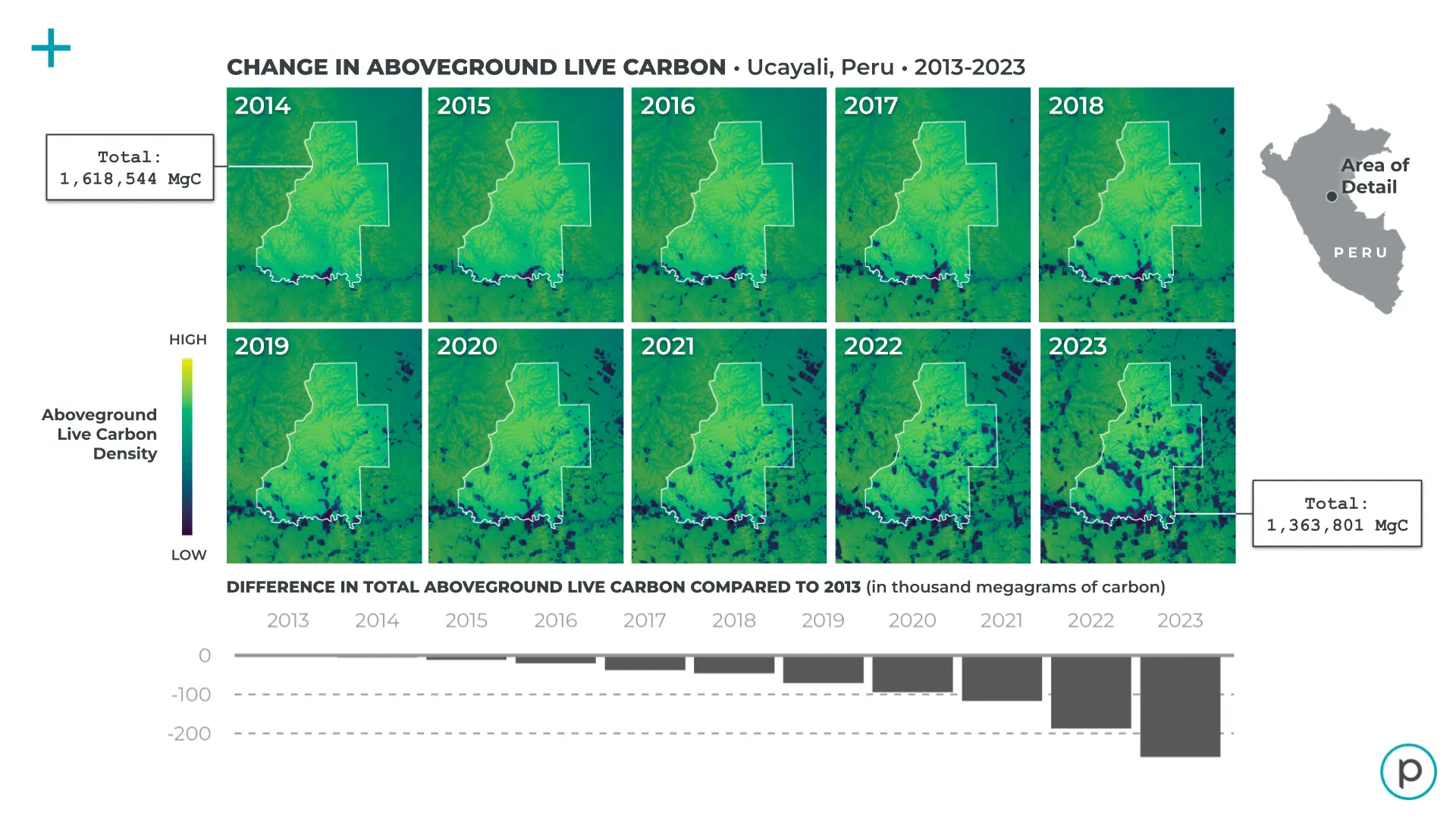
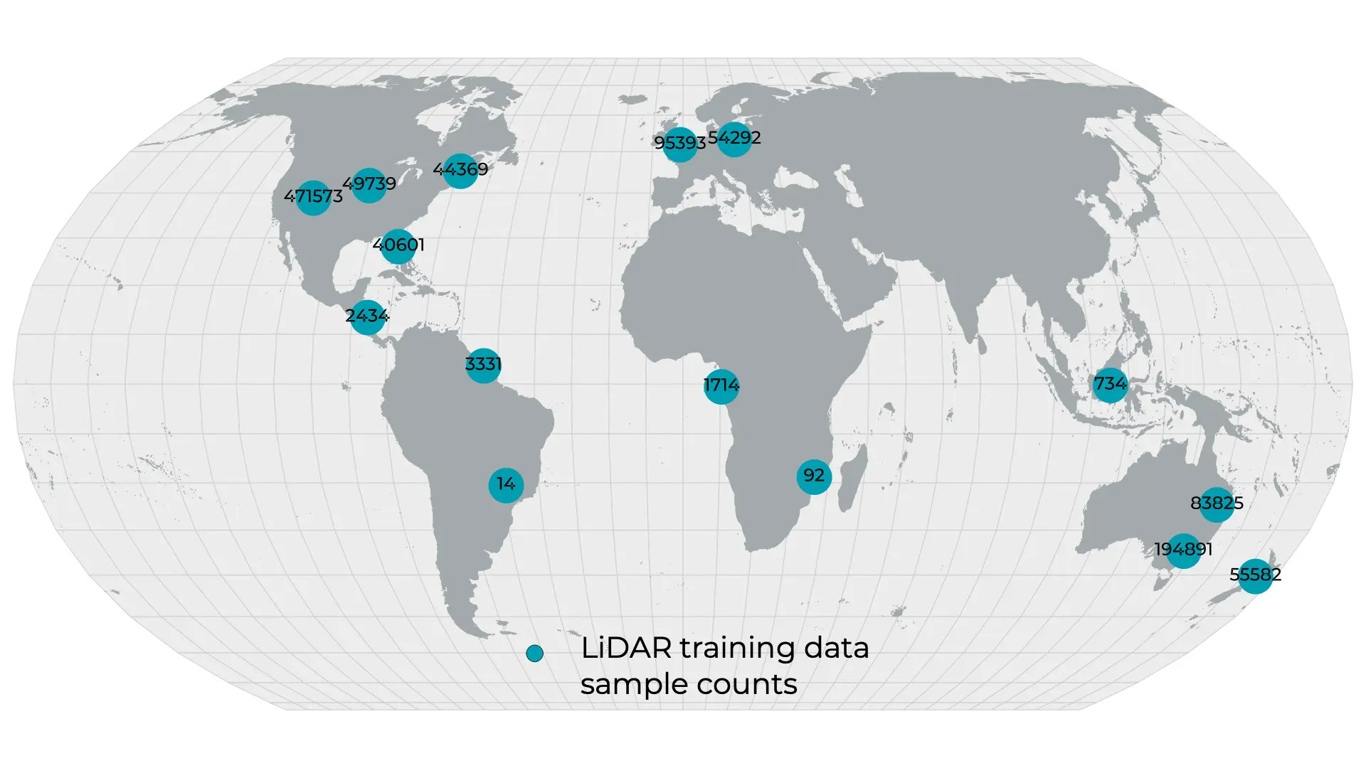
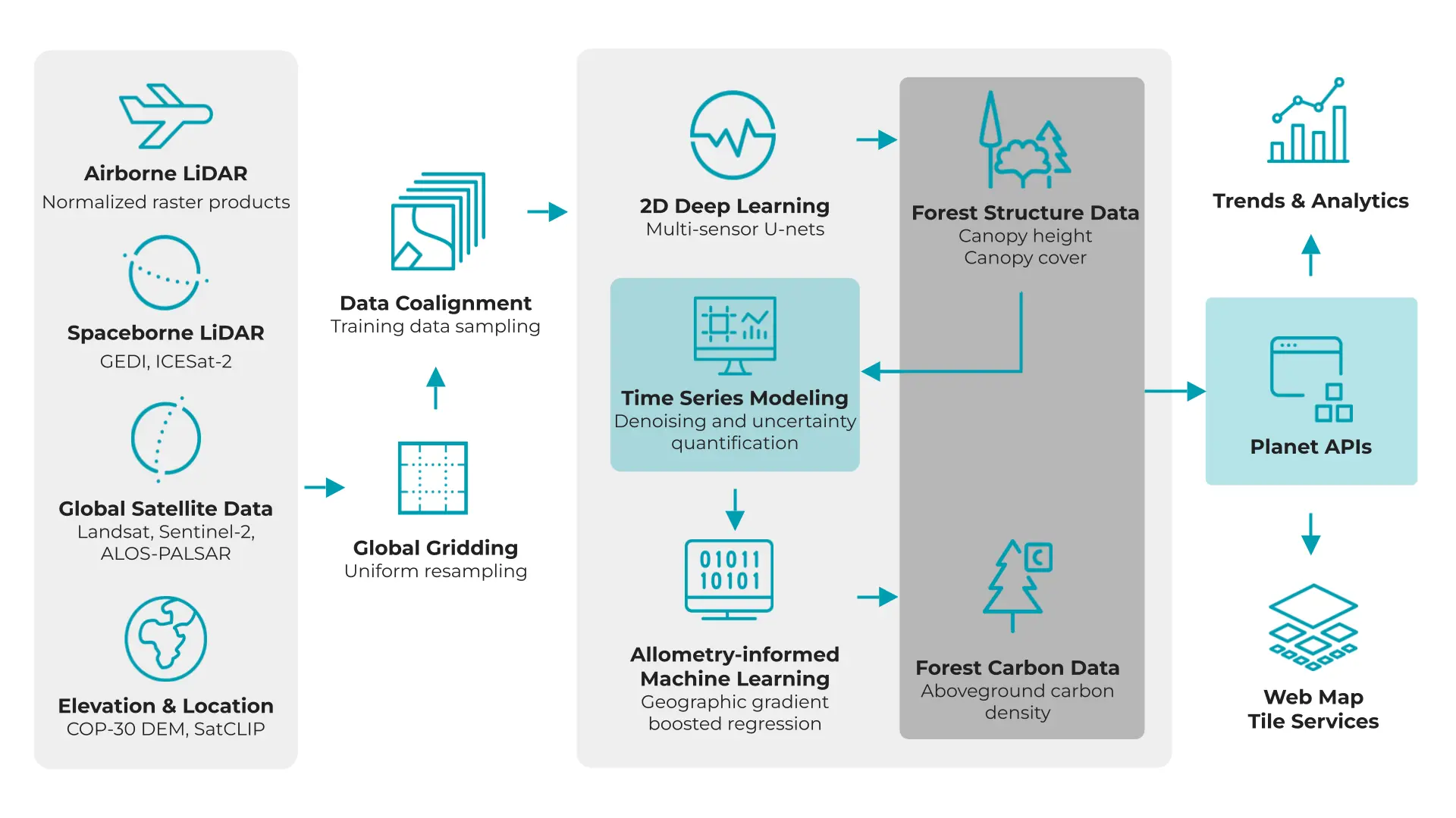
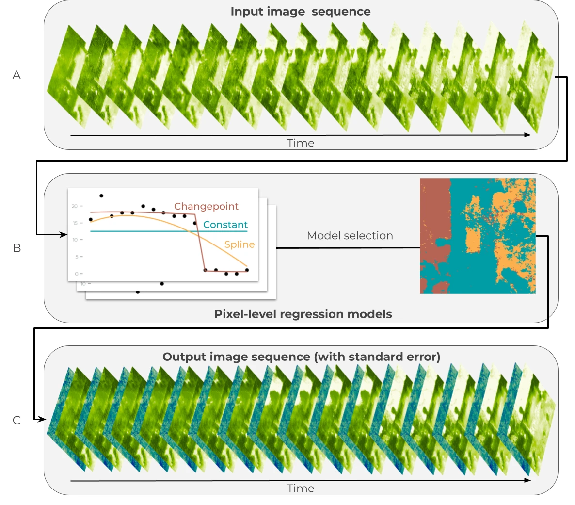
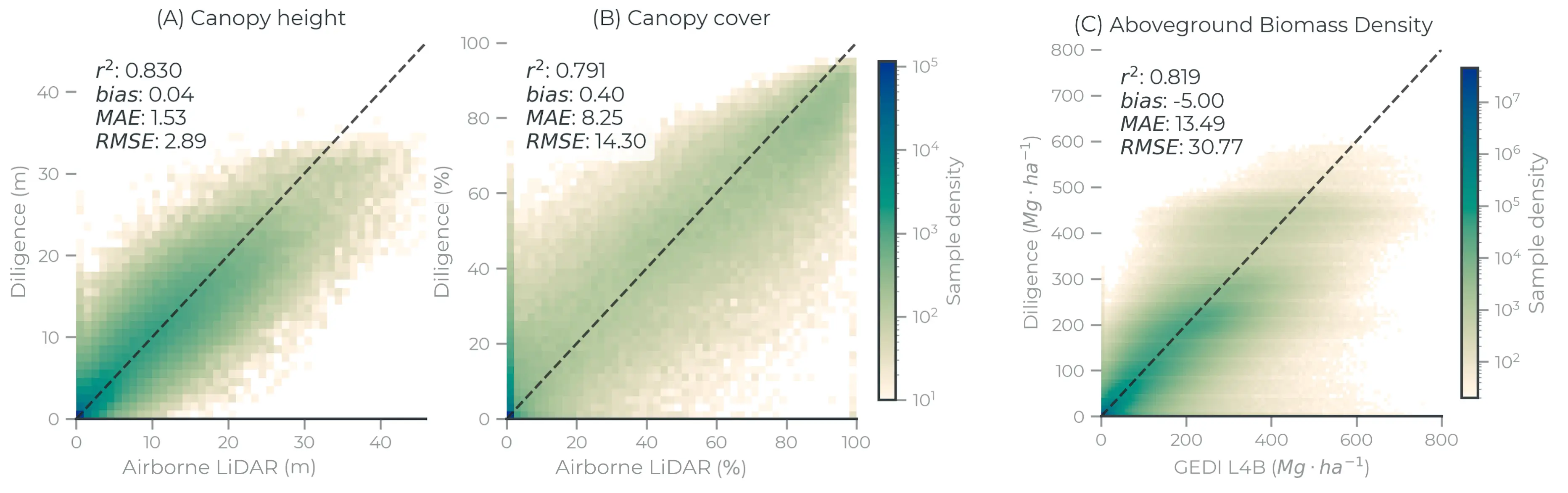

20km² [Visualize in the Browser →](https://insights.planet.com/analyze/browser/?zoom=14\&lat=17.1481\&lng=105.82251\&themeId=PLANET_SANDBOX\&visualizationUrl=U2FsdGVkX1%2Fa%2Bw4wG8eIVfMgk%2FvDmhHxrovEwT%2FEvdBTkh4WvmXCd68%2Fq06VUwKIkmD5TMpuNJSzHZ6vxk3aqMvRO%2FyXNDbNLXZoCl0eD8yclCUNEhnG53w9KwWdSo%2Fe\&datasetId=d4a2a179-0c1a-4426-8d54-e2ac82830e83\&fromTime=2023-09-21T00%3A00%3A00.000Z\&toTime=2023-09-21T23%3A59%3A59.999Z\&layerId=ABOVEGROUND-CARBON-DENSITY\&demSource3D="MAPZEN") [![Atsimo-Andrefana, Madagascar](/data/planetary-variables/forest_carbon_monitoring/FCM_MADAGASCAR.webp)](https://insights.planet.com/analyze/browser/?zoom=14\&lat=-22.2323\&lng=43.78691\&themeId=PLANET_SANDBOX\&visualizationUrl=U2FsdGVkX180XBAZynT8rOzF%2BQ44Xiaw0jjWE8kZ4I4pmiR8Z9sTnzKRpS3xqSik8pvp2FciGQyx1D8A9ooKBbyeflbMS55w3D%2FaBiRog85G13XWTnBALO%2BDzwYhV60n\&datasetId=ca501757-cf8e-43a8-b1a4-1aa59ae22425\&fromTime=2023-09-21T00%3A00%3A00.000Z\&toTime=2023-09-21T23%3A59%3A59.999Z\&layerId=CANOPY-COVER\&demSource3D="MAPZEN") Atsimo-Andrefana, Madagascar 2020-12-21 - 2023-09-21
26km² [Visualize in the Browser →](https://insights.planet.com/analyze/browser/?zoom=14\&lat=-22.2323\&lng=43.78691\&themeId=PLANET_SANDBOX\&visualizationUrl=U2FsdGVkX180XBAZynT8rOzF%2BQ44Xiaw0jjWE8kZ4I4pmiR8Z9sTnzKRpS3xqSik8pvp2FciGQyx1D8A9ooKBbyeflbMS55w3D%2FaBiRog85G13XWTnBALO%2BDzwYhV60n\&datasetId=ca501757-cf8e-43a8-b1a4-1aa59ae22425\&fromTime=2023-09-21T00%3A00%3A00.000Z\&toTime=2023-09-21T23%3A59%3A59.999Z\&layerId=CANOPY-COVER\&demSource3D="MAPZEN") [![Idaho, USA](/data/planetary-variables/forest_carbon_monitoring/FCM_USA.webp)](https://insights.planet.com/analyze/browser/?zoom=13\&lat=47.70965\&lng=-116.34633\&themeId=PLANET_SANDBOX\&visualizationUrl=U2FsdGVkX1%2B8RQf7awJj1vqgAQjivr9mg3%2FjJskyAAugtAOVN9ARX24T1EVtjuDj5K2e2IIUVW6%2FNtCZBQPVqsaPDbZYlF4cFwsfsmNnc7W94%2BF7ISJa8ivVLR7aFFsM\&datasetId=d09d8fd8-a3b3-49fb-9d78-47f3a5cc8ecc\&fromTime=2023-09-21T00%3A00%3A00.000Z\&toTime=2023-09-21T23%3A59%3A59.999Z\&layerId=CANOPY-HEIGHT\&demSource3D="MAPZEN") Idaho, USA 2020-12-21 - 2023-09-21
20km² [Visualize in the Browser →](https://insights.planet.com/analyze/browser/?zoom=13\&lat=47.70965\&lng=-116.34633\&themeId=PLANET_SANDBOX\&visualizationUrl=U2FsdGVkX1%2B8RQf7awJj1vqgAQjivr9mg3%2FjJskyAAugtAOVN9ARX24T1EVtjuDj5K2e2IIUVW6%2FNtCZBQPVqsaPDbZYlF4cFwsfsmNnc7W94%2BF7ISJa8ivVLR7aFFsM\&datasetId=d09d8fd8-a3b3-49fb-9d78-47f3a5cc8ecc\&fromTime=2023-09-21T00%3A00%3A00.000Z\&toTime=2023-09-21T23%3A59%3A59.999Z\&layerId=CANOPY-HEIGHT\&demSource3D="MAPZEN") --- Copy for LLM[View as Markdown](https://docs.planet.com/data/planetary-variables/forest-carbon-monitoring/techspec/) # Technical Specification ![Figure 1: Side-by-side view of PlanetScope Mosaics and aboveground carbon density data over the Amazon River in Amazonas, Brazil.](/data/planetary-variables/forest_carbon_monitoring/fcm_basemap_acd.webp) Figure 1: Side-by-side view of PlanetScope Mosaics and aboveground carbon density data over the Amazon River in Amazonas, Brazil. Forest Carbon Monitoring provides a series of data products for mapping forest change at high resolution worldwide. These products provide timely, operational insights into changes in canopy cover, canopy height, and aboveground carbon density with unprecedented detail, powered by Planet’s unique imaging constellation. The initial release includes quarterly observations starting in December 2020, providing rolling insights into forest structure and carbon. The Forest Carbon Monitoring products were primarily designed to support project and jurisdictional MRV1, as well as supply chain risk evaluations for EUDR2 compliance. The leading project type in carbon markets follows the REDD+3 framework of avoiding deforestation, and Forest Carbon Monitoring excels at tracking forest loss at fine scales and quantifying the resulting carbon losses. The power of quarterly, high resolution data is in detecting complex, diffuse patterns like degradation and regrowth. Not all forest loss is uniform, and it is crucial to map the selective harvests of individual trees or small groups of trees in order to accurately estimate forest inventories at scale. While detecting changes early in a tree's life history is often challenging, Forest Carbon Monitoring is sensitive to young tree growth. These data can be combined with in situ data for digital MRV of natural regeneration or explicit ARR4 interventions. When scaled up to sub-national or national scales, Forest Carbon Monitoring can support jurisdictional carbon accounting and policy implementations related to land-based climate mitigation. Acronyms 1. MRV: Monitoring, reporting and verification 2. EUDR: European Union Deforestation Regulation 3. REDD+: Reducing emissions from deforestation and forest degradation 4. ARR: Afforestation, reforestation and restoration ## Product Specifications Table 1: Forest Carbon Monitoring product specification | Specification | Value | | ------------------- | ------------------------------------------------------- | | Metrics | Canopy cover, canopy height, aboveground carbon density | | Spatial extent | Global land mass > -60S and < 75N, excluding ice sheets | | Temporal extent | Dec. 2020 - Present | | Temporal resolution | Quarterly | | Temporal periods | Q1: Dec 21 - Mar 20 | | | Q2: Mar 21 - Jun 20 | | | Q3: Jun 21 - Sep 20 | | | Q4: Sep 21 - Dec 20 | Canopy cover (CC) quantifies the percentage of area occupied by trees within a pixel, where a tree is defined as vegetation 5 meters or taller. This metric will be most sensitive to tree loss events like timber harvest or deforestation, and to increases in tree cover due to regeneration or ARR. Canopy height (CH) quantifies the average top-of-canopy height within each pixel. While this metric is sensitive to tree loss, it is less sensitive to large tree growth. Vertical growth is typically slower in mature trees compared to young trees, meaning quarter-over-quarter height increases are not frequently observed outside of regrowth contexts. Aboveground carbon density (ACD) quantifies the expected density of carbon stored in woody biomass, measured in units of mass per area (megagrams of carbon per hectare). It is not a direct estimate of the total carbon in each pixel or each tree, but an estimate of area-based carbon density. ## Asset Properties This tables specifies the properties of the data assets delivered by the [Planet Subscriptions API](https://docs.planet.com/develop/apis/subscriptions.md). Table 2: Forest Carbon Monitoring data resource properties | Metric | Asset Name | Units | Type | Typical Range | No Data Value | Band Count | Resolution | | -------------------------- | ---------- | ----- | ----- | ------------- | ------------- | ---------- | ------------------- | | Canopy Cover | cc | % | UINT8 | 0 - 100 | 255 | 1 | 0.000025° (±3x3 m) | | Canopy Height | ch | m | UINT8 | 0 - 50 | 255 | 1 | 0.000025° (±3x3 m) | | ACD: Minimum Mapping Unit | acd-mmu | Mg/ha | INT16 | 0 - 300 | 32767 | 1 | 0.00025° (±30x30 m) | | ACD: Downscaled | acd | Mg/ha | INT16 | 0 - 300 | 32767 | 1 | 0.000025° (±3x3 m) | | CC Uncertainty | cc-uc | % | UINT8 | 0 - 100 | 255 | 2 | 0.000025° (±3x3 m) | | CH Uncertainty | ch-uc | m | UINT8 | 0 - 80 | 255 | 2 | 0.000025° (±3x3 m) | | ACD MMU Uncertainty | acd-mmu-uc | Mg/ha | INT16 | 0 - 300 | 32767 | 2 | 0.00025° (±30x30 m) | | ACD Downscaled Uncertainty | acd-uc | Mg/ha | INT16 | 0 - 300 | 32767 | 2 | 0.000025° (±3x3 m) | Aboveground carbon density data are provided at two spatial resolutions. The 30m Minimum Mapping Unit (MMU) data estimates carbon density at the native resolution of the model. This product is straightforward to analyze and validate, and aligns with best mapping practices recommended by the [Committee on Earth Observing Systems](https://lpvs.gsfc.nasa.gov/PDF/CEOS_WGCV_LPV_Biomass_Protocol_2021_V1.0.pdf) (CEOS). The 3m Downscaled product provides carbon estimates that match the resolution of the canopy height and canopy cover products. The value of downscaled data is to quantify carbon density over small—but not sub-tree—areas, like smallholder farms, selective harvests, field plots, and carbon projects. Because the downscaled data are provided at a spatial resolution finer than the size of most tree crowns, downscaled carbon estimates should be aggregated across multiple pixels, which greatly improves prediction quality and interpretability. This product empowers users to flexibly aggregate data to the scales that fit their needs, particularly in use cases where coarse, gridded data pose analytical challenges. See the [Carbon Downscaling Method](#carbon-downscaling) section for more details on the downscaling approach, and the [Minimum Mapping Units](#minimum-mapping-units) section for guidance on aggregation. Table 3. Uncertainty band descriptions | Uncertainty band | Description | | ---------------- | ---------------------------------------- | | Q05 (band 1) | Lower prediction bound (5th percentile) | | Q95 (band 2) | Upper prediction bound (95th percentile) | Uncertainty data are provided as calibrated 90% prediction intervals for each pixel in each quarter. These values are provided in the same units as their respective reference data. In other words, the pixel values and units are consistent between the "cc" and "cc-uc" assets. ### Input Data Canopy height and canopy cover are estimated at high resolution using computer vision models. Airborne LiDAR data are the response variables, and a series of satellite-derived datasets are the feature variables. Forest carbon density is first estimated at 30m resolution using a gradient boosting regression model, then downscaled using a linear [downscaling model](#carbon-downscaling). GEDI L4A data are the response variable, and canopy height, canopy cover, and elevation data are the feature variables. Table 4: List of inputs for Forest Carbon Monitoring production | Product | Description | | ----------------------------- | ------------------------------------------------------------------------------------------------------------------------------------------------------------------------------------------------------------------------------ | | Airborne LiDAR | Point cloud data processed to rasters of canopy height and canopy cover at 1m resolution, then resampled to match the Surface Reflectance data. | | GEDI L4A | [GEDI L4A](https://doi.org/10.3334/ORNLDAAC/1907) data encode modeled estimates of aboveground biomass density across most of the terrestrial biosphere. | | Surface Reflectance | Quarterly, 4-band [PlanetScope Surface Reflectance Mosaics](https://assets.planet.com/products/basemap/planet-basemaps-product-specifications.pdf), spectrally normalized to Sentinel-2. | | Forest Carbon Diligence | 30m canopy height and canopy cover data from the [Forest Carbon Diligence](https://planet.widen.net/s/rv77kqctqw/planet-userdocumentation-forestcarbon) product. | | Digital Elevation Model (DEM) | Copernicus [GLO-30](https://doi.org/10.5270/ESA-c5d3d65) DEM are used for most of the global landmass, ALOS [AW3D30](https://www.eorc.jaxa.jp/ALOS/en/dataset/aw3d30/aw3d30_e.htm) is used where GLO-30 does not provide data. | ## Methods ![Figure 2: Workflow diagram for Forest Carbon Monitoring illustrating the flow of data for delivery.](/data/planetary-variables/forest_carbon_monitoring/fcm_overview_conceptual.webp) Figure 2: Workflow diagram for Forest Carbon Monitoring illustrating the flow of data for delivery. ### Global Gridding and Co-alignment A global grid was used to create deterministic, geographically independent samples, assigned to non-overlapping sets for model training, validation, and testing. This grid was specified using the [EASE Grid 2.0](https://doi.org/10.3390/ijgi1010032) equal area projection (EPSG:6933) at 3.4m resolution. EASE Grid offers an efficient layout design, storing only 60% of the pixel count compared to a geographic coordinate system at a comparable resolution. This cylindrical projection preserves area but distorts shapes close to the poles, which could introduce spatial artifacts in the vision model. A large amount of training data was acquired at high latitudes to mitigate this effect. Training data was generated by randomly sampling 128x128 pixel tiles from regions with high quality airborne LiDAR data, and a deterministic grid was used to define the sampling strategy. First, the grid was overlaid with the LiDAR extent, and tile centroids were sampled over non-overlapping valid data locations. Once the tile locations were selected, a coarser grid was used to split data into training, validation, and testing groups. 2x2 quads were split so that samples within two of the tiles were used for model training, one for validation, and one for testing. This resulted in an approximately 50-25-25 split with no spatial overlap between tiles. In total, this produced 27.5 million hectares of data for training and evaluation, with 806,826 samples used for training, 253,497 for validation, and 352,870 for testing. Quarterly, 4-band surface reflectance mosaics were produced starting in 2018 based on the quality and quantity of available PlanetScope data. Surface reflectance and LiDAR data were time matched to select temporally-coincident observations. LiDAR data collected prior to 2018 was matched to the 2018 surface reflectance mosaic. For LiDAR data with large or imprecise collection periods, the nearest leaf-on quarter was selected (corresponding to spring in the northern and southern hemisphere). Training data were spatially resampled to align in shape and resolution. Each sample was a 128x128 array at 3.4m resolution, projected to EASE Grid. The response data—LiDAR-derived canopy height and canopy cover—were average resampled to this scale. The feature data—surface reflectace mosaics and the 30m Forest Carbon Diligence data—were extracted with nearest-neighbor resampling then concatenated in the channel dimension, creating a 6-band feature stack. Diligence data from the time-matched year was selected for each sample. The Diligence data were included to provide contextual information to the model regarding the absolute canopy height and canopy cover values for each sample, and to improve alignment across products. ### 2D Deep Learning U-Net image regression models were trained to predict canopy height (m) and canopy cover (%) at 3.4m resolution, using surface reflectance mosaics and 30m maps of height and cover as predictors. The height and cover response datasets were modeled simultaneously in a multi-task learning framework using Joint Task Training ([Crenshaw 2020](https://doi.org/10.48550/arXiv.2009.09796)). This approach optimized both accuracy and efficiency. There is strong but non-linear covariance between canopy height and canopy cover, and many of the spectral features used to estimate these patterns are shared across contexts, leading to efficient model training convergence. Including canopy height and canopy cover maps from the Diligence product increased the overall feature dimensionality, improving predictive power. Sharing a joint encoder/decoder also improved consistency in the output prediction features, so post-processing harmonization was unnecessary. Multi-task learning reduced the overall saturation of canopy height predictions, increasing the predicted heights at the tall end of the distribution, though these effects are [still pronounced](#canopy-height-saturation). The U-Net model architecture was modified to include ResNet blocks and a series of network-in-network connections ([Lin et al. 2013](https://doi.org/10.48550/arXiv.1312.4400), [Zhang et al. 2018](https://doi.org/10.1109/LGRS.2018.2802944)). The Log Cosh loss function was used to minimize the contributions of large residual errors to model convergence, which was found to improve canopy height predictions. Using spatially-independent validation data—instead of shuffling training and validation data at runtime—was found to improve model generalization, minimizing the difference between training and testing metrics. Model inference was applied independently to each quarter's feature stack. As a result, seasonal vegetation patterns and sun-sensor observation variability introduce quarter-over-quarter variance to the raw model predictions. Experiments found that training models with just leaf-on observations improved generalization across quarters, compared to models trained using both leaf-on and leaf-off observations. This quarter-over-quarter variance is addressed downstream using time series models. ### Time Series Modeling ![Figure 3: Statistical modeling for estimating canopy height and canopy cover over time. (A) An image time series is generated from the raw predictions of the vision model for times t=1, … T. (B) Three regression models are fit for each pixel: a constant model to represent the temporal mean (blue), a changepoint model to represent sudden change (red), and a spline model to represent gradual change (orange). A model is selected for each pixel, with the preferred model color coded in the image on the right. (C) The preferred model for each pixel is used to generate denoised predictions for each time step: expected values (green color ramp) and standard errors of the predictions (blue color ramp).](/data/planetary-variables/forest_carbon_monitoring/fcm_denoising_conceptual.webp) Figure 3: Statistical modeling for estimating canopy height and canopy cover over time. (A) An image time series is generated from the raw predictions of the vision model for times t=1, … T. (B) Three regression models are fit for each pixel: a constant model to represent the temporal mean (blue), a changepoint model to represent sudden change (red), and a spline model to represent gradual change (orange). A model is selected for each pixel, with the preferred model color coded in the image on the right. (C) The preferred model for each pixel is used to generate denoised predictions for each time step: expected values (green color ramp) and standard errors of the predictions (blue color ramp). The vision model predicts height and cover for each quarter independently, and the predictions contain variation related to phenology, illumination, and sensor calibration. We minimize the variation in prediction sequences using statistical models. For each pixel, three models are fit: 1. A constant-in-time model, which represents stability over time 2. A spline model, which represents gradual change 3. A changepoint model, which represents fast change The constant-in-time model assumes that all variation in predictions is due to noise. This model is expected to perform well when height or cover remains stable over time or when changes are minimal relative to the noise in the predictions (for example, slow growth that is not detectable over a few years). The spline and changepoint models are designed to capture slow and fast changes, respectively. Regularized B-splines are used to estimate non-linear trends, while the changepoint model includes a discrete change point parameter at the timestep with the greatest change in predicted height or cover. The preferred model for each pixel is selected using Akaike's Information Criteria (AIC). An additional heuristic is applied to reduce noise: if the coefficient of variation (over time) for the preferred model's predictions is below a threshold, the constant-in-time model is selected. This coefficient of variation threshold is a hyperparameter tuned alongside the AIC threshold. Once a preferred model is selected for each pixel, predictions are generated and predictive error is quantified using the standard errors of predicted values from the regression models. These standard errors are used downstream to quantify pixel-level uncertainty for height and cover. ### Carbon Downscaling ![Figure 4: Overview of 3m aboveground carbon estimation. First, 3m height and cover data are average resampled to 30m. The 3m and 30m data are then provided separately as inputs to the AGC model (natively trained at 30m). This produces 3m and 30m carbon predictions. To ensure that the average of 3m AGC data equals the average of the 30m data, we apply a scale adjustment to the 3m data based on the ratio of 30m and unscaled 3m means.](/data/planetary-variables/forest_carbon_monitoring/fcm_downscaling_conceptual.webp) Figure 4: Overview of 3m aboveground carbon estimation. First, 3m height and cover data are average resampled to 30m. The 3m and 30m data are then provided separately as inputs to the AGC model (natively trained at 30m). This produces 3m and 30m carbon predictions. To ensure that the average of 3m AGC data equals the average of the 30m data, we apply a scale adjustment to the 3m data based on the ratio of 30m and unscaled 3m means. Aboveground carbon density estimates are generated at 3m nominal resolution using statistical downscaling. This downscaling approach is designed to satisfy two criteria: 1. At fine scales, carbon estimates should be consistent with 3m height and cover. 2. At large scales, aggregated 3m carbon estimates should be consistent in expectation with 30m carbon estimates. Simple linear downscaling of a model trained at 30m is used to meet these criteria. This 30m model is trained on L4A aboveground biomass estimates derived from NASA's Global Ecosystem Dynamics Investigation (GEDI) spaceborne lidar sensor. Given height and cover estimates, the model can predict aboveground biomass, which is converted to aboveground carbon by multiplying by a scalar representing the global mean carbon concentration. The details on model training, model performance, and scaling is described in more detail in the [Forest Carbon Diligence Technical Specification](https://planet.widen.net/s/rv77kqctqw/planet-userdocumentation-forestcarbon). 30m is considered the "native scale" of the carbon model. To create 3m estimates from the 30m model, 3m height and cover are passed as inputs, generating raw 3m carbon predictions. These predictions are "raw" due to the scale mismatch between the model's training resolution (30m) and the deployment resolution (3m). Next, 3m height and cover are average resampled to 30m, and the 30m height and cover inputs are passed to the model to create 30m carbon estimates at the native resolution. Mean carbon is then computed for both the raw 3m and native 30m predictions, and the ratio of means is used to compute a scale adjustment. Final 3m carbon predictions are computed by scaling raw 3m carbon estimates, ensuring that the average carbon of the 30m predictions equals the average carbon of the final 3m predictions. ### Pixel-level Uncertainty Standard errors from the pixel-level time series models are used to construct 90% prediction intervals for height and cover. Intervals are constructed as: $[y_{pred} - \widehat{q} \cdot \sigma_{pred}, y_{pred} + \widehat{q} \cdot \sigma_{pred}]$ where $y_{pred}$ is a predicted value from the time series model, $\sigma_{pred}$ is the standard error of the prediction, and $\widehat{q}$ is a parameter estimated using withheld data via split conformal inference. Split conformal inference uses disjoint partitions of a dataset to produce well-calibrated prediction intervals. These are 90% prediction intervals that contain the true value approximately 90% of the time ([Angelopolous and Bates 2021](https://doi.org/10.48550/arXiv.2107.07511)). A calibration dataset is used to estimate $\widehat{q}$, a scalar quantity that determines the width of the interval relative to the standard error to achieve 90% coverage. After generating predictions with $\widehat{q}$, empirical interval coverage is quantified on a spatially non-overlapping test set. Test set coverage was 90.3% for canopy cover and 91.7% for canopy height. ## Data Quality ### Deep Learning Model Performance ![Figure 5: Scatter plots for canopy height predictions at 3m (left), 10m (middle) and 30m (right) resolutions.](/data/planetary-variables/forest_carbon_monitoring/fcm_scatterplots_canopyheight.webp) Figure 5: Scatter plots for canopy height predictions at 3m (left), 10m (middle) and 30m (right) resolutions. There are several drivers of prediction uncertainty, including model variance, observation quality, and orthorectification quality. These drivers are difficult to disentangle, but we provide a comparison of multi-scale model performance below to illustrate how model performance improves with aggregation. Users are encouraged to analyze the data at the scale that fits their analysis. This is often at the original scale of the data. But in contexts where prediction accuracy is critical, aggregating forest structure data provides meaningful improvmeents. High resolution data is valuable beyond providing detailed maps; aggregating high resoultion data can capture subtle, fine-scale dynamics more precisely at scale than direct observations at lower resolution. Table 5. Multi-scale model performance comparison | Metric | Resolution | R2 | MAE | RMSE | | ------------- | ---------- | ---- | ---- | ---- | | Canopy height | 3m | 0.68 | 2.4m | 4.2m | | | 10m | 0.75 | 1.9m | 3.4m | | | 30m | 0.81 | 1.6m | 2.9m | | Canopy cover | 3m | 0.70 | 12% | 20% | | | 10m | 0.78 | 9% | 16% | | | 30m | 0.84 | 7% | 12% | ### Canopy Height Saturation ![Figure 6: Binned residual error plots for canopy height show attenuated signal for taller trees. The residual errors for each test data observation were binned in 5 meter increments for this box plot, showing canopy height predictions are systematically lower for tall trees. This plot is not normalized by sample frequency.](/data/planetary-variables/forest_carbon_monitoring/fcm_residuals_canopyheight.webp) Figure 6: Binned residual error plots for canopy height show attenuated signal for taller trees. The residual errors for each test data observation were binned in 5 meter increments for this box plot, showing canopy height predictions are systematically lower for tall trees. This plot is not normalized by sample frequency. Signal saturation is a well-known challenge to estimating canopy height using optical satellite data ([Mutanga et al., 2023](https://doi.org/10.1016/j.isprsjprs.2023.03.010)). This refers to the limited signal available in optical remote sensing data to predict tree heights beyond 25-30 meters above ground. While several modeling approaches were tested to minimize this effect (see [2D Deep Learning](#2d-deep-learning)), it remains visible in the residual error plots (Figure 6). This might pose a challenge for users who depend on unbiased canopy height estimates (in allometric regression models, for example). In empirical use cases, signal saturation may not be as problematic. For example, the aboveground carbon density model used in this product estimates empirical relationships between predicted canopy height and canopy cover maps and the observed carbon density data. Practically, this results in strong model performance for the low and mid range of carbon estimates, though predictions in the most carbon-dense forests will likely be underestimated. ![Figure 7: Residual error histograms for canopy height (left) and canopy cover (right).](/data/planetary-variables/forest_carbon_monitoring/fcm_histograms_structure.webp) Figure 7: Residual error histograms for canopy height (left) and canopy cover (right). Overall, the deep learning model converged to predict both canopy height and canopy with low total bias across the full test data set. Although there is signal saturation among taller trees, higher predictions at lower heights balance the overall predictions, driving low population-level bias. This effect further demonstrates the value of spatial aggregation. While bias may occur at any one point across the landscape, these biases decrease with aggregation, and the total bias over large areas is likely to be low. ### Minimum Mapping Units The aboveground carbon density products are provided at multiple spatial resolutions: 30m and 3m. The reason for providing multiple assets is related to a geographic concept known as the minimum mapping unit. [Knight and Lunetta, 2003](https://doi.org/10.1109/TGRS.2003.816587) provide a short review of this topic. The minimum mapping unit for forest carbon products refers to the smallest area over which carbon estimates can be reliably quantified and validated. Because the forest carbon data were fit using [GEDI L4A](#input-data) data and 30m feature data, the minimum mapping unit for the carbon model is 30m. This is approximately the size of a 0.1 ha field plot. Although the downscaled product is provided at 3m resolution—which can be smaller than the size of an individual tree—the minimum mapping unit for analysis remains 30m. So why provide a data product at a scale finer than the minimum mapping unit? The primary value proposition of high resolution data is to provide a flexible data product that can be aggregated to the appropriate scale of analysis, which varies by use case. Current best practices recommend mapping carbon at 0.25 - 1 ha (50 - 100m) resolution in tropical forests, and 0.1-0.25 ha (30 - 50m) in boreal and temperate forests ([CEOS 2021](https://lpvs.gsfc.nasa.gov/PDF/CEOS_WGCV_LPV_Biomass_Protocol_2021_V1.0.pdf), [Frazer et al. 2011](https://doi.org/10.1016/j.rse.2010.10.008)). The Food and Agriculture Organization (FAO) developed a consensus forest definition, which specified minimum thresholds of areas with 10% canopy cover, 5 m tree height, covering at least 0.5 ha ([FAO 2000](https://www.fao.org/forest-resources-assessment/fra-2000/en)). Aggregation to 1 ha has been shown to minimize prediction uncertainty and identified as the optimal scale for accurately estimating forest carbon stocks from remote sensing ([Mascaro et al. 2011](https://doi.org/10.1016/j.rse.2011.07.019), [Chen et al. 2016](https://doi.org/10.1016/j.rse.2016.07.023)). While each of these scales is greater than the 0.1 ha minimum mapping unit, data provided at that resolution may still prove prohibitive. Scale mismatches between field and satellite datasets has long been one of the primary drivers of uncertainty and barriers to effective validation, especially when validating plots that may only be one or two pixels in size or fall on borders between pixels ([Wu and Li, 2009](https://doi.org/10.3390/s90301768), [Anderson 2018](https://doi.org/10.1111/ele.13106), [Réjou-Méchain et al. 2019](https://doi.org/10.1007/s10712-019-09532-0)). Mismatches between satellite resolution and forest definitions make global forest change analysis prohibitively complex, too. This has become so acute that some researchers have called to change the FAO's global definition of forests to instead be defined by the 30m resolution of Landsat ([Zalles et al. 2024](https://doi.org/10.1038/s43247-024-01779-9)). Instead of asking users to redefine their problems to accomodate their data, the downscaled product was developed to accomodate the wide range of contexts our users work in. It is straightfoward to resample the downscaled product over field plots, carbon projects, disturbed areas, or tree planting sites. The carbon estimates will be valid so long as the data are aggregated to at least the minimum mapping unit. To demonstrate the value of high resolution carbon data, consider the case of carbon quantification over smallholder farms. Recent work found that smallholder farmers in Rwanda planted an average of 3 trees per farm over a decade of analysis, which added up to over 50 million new trees nation-wide ([Mugabowindekwe et al. 2024](https://doi.org/10.1038/s43247-024-01278-x), [Brandt et al. 2024](https://doi.org/10.1038/s44287-024-00116-8)). Individually, these contributions to a national carbon budget are minimal, and may not be detectible from lower resolution observations. But a full accounting of smallholder contributions could prove meaningful at jurisdictional scales. Developing cost-effective MRV tools for quantifying changes in carbon stocks was identified as a top priority for engaging smallholder farmers in carbon markets, and high resolution data uniquely addresses this need ([Schilling et al. 2023](https://hdl.handle.net/10419/278420)). The 3m downscaled forest carbon product was not developed to provide sub-tree estimates of carbon density; it was designed to empower users to flexibly aggregate data to the scales that fit their needs, particularly in use cases where coarse, gridded data pose analytical challenges. The 30m MMU product supports direct carbon stock analyses, requiring no additional modifications by uses to derive meaningful carbon estimates. Both products should be analyzed at a minimum mapping unit of 30m, though that does not preclude aggregation to the appropriate scale of analysis for your use case. ## Known Issues **Halo effects**. The time series model estimates forest structure patterns across the full temporal extent of data and updates all predictions simultaneously. This can create visually-distinct boundaries between areas where rapid changes were observed, which propagate back in time. As a result, post-change edge effects can appear in the data prior to the observed vegetation change. This will typically be captured by the pixel-level prediction intervals, showing higher prediction uncertainty on the borders of disturbances. Anecdotally, this effect appears to be largely visual, with low numerical differences. **Pixel coregistration**. PlanetScope surface reflectance data are provided with some positional uncertainty, meaning pixel locations may shift slightly quarter-over-quarter. PlanetScope absolute positional uncertainty is quantified in Section 3.3 in the [Imagery Product Specification](https://assets.planet.com/docs/Planet_Combined_Imagery_Product_Specs_letter_screen.pdf). Practically, this presents as a slight decrease in pixel-level contrast, and predictions may not appear as crisp as expected. **False positive changes in the most recent time step**. The time series model is an effective outlier filter, smoothing over noisy observations from unmasked clouds, snow, or missing data. These models rely on additional observations that follow the noisy observations, which indicate a change did not persist. Additional observations are not available for the most recent time step, which increases the rate of false positive changes. For time-sensitive use cases, we advise users to consult the uncertainty layer, which should show high uncertainty in areas with anomalous change. For less time-sensitive use cases, we advise using the previous quarter's data to minimize false positives. The most recent quarter's data will be updated once new observations are available to correct these issues. **Most changes are observed at year-to-year boundaries**. Including the annual, 30m Forest Carbon Diligence data as predictive features improves prediction accuracy but introduces a temporal mismatch in production. New Diligence observations are included at Q1 of each year, but are not updated for each following quarter. Changes detected from Diligence—both growth and loss—may not be captured until the next year. This means that change detection primarily occurs at year-to-year boundaries when new 30m observations are included. --- Copy for LLM[View as Markdown](https://docs.planet.com/data/planetary-variables/forest-carbon-monitoring/validation/) # Validation Report Coming soon --- Copy for LLM[View as Markdown](https://docs.planet.com/data/planetary-variables/land-surface-temperature/) # Land Surface Temperature ![Header Thumbnail](/data/planetary-variables/land-surface-temperature/lst_thumbnail.webp) Accurate monitoring of Earth's surface temperature through satellite-derived information supports the understanding of many of our planet’s ecosystems, including physical processes that govern the three major cycles: carbon, energy and water. Leveraging multiple earth observation datasets and innovative patented technology, Planet provides a twice-daily, global, consistent and accurate Land Surface Temperature products. These datasets are not just numbers; It is a valuable tool for monitoring changes in cities, or understanding plant health and water availability. Also, this data plays a crucial role in assessing climate and meteorological risks by tracking temperature anomalies and shifts over time using the long archive capability. What makes the Planet Land Surface Temperature (LST) product stand out is its unique blend of microwave and optical data, allowing the observation of temperature regardless of the cloud condition, so data can be compared consistently over time and space, providing the detailed insights needed for various applications. ## Use Cases **Crop Stress Monitoring** - Using LST as input in energy balanced-based evaporation models, crop stress can be detected early on and allows early intervention. **Phenology development** - LST can be used as input for Growing Degree Days ([check out the blog post](https://www.planet.com/pulse/satellite-based-land-surface-temperature-for-deriving-growing-degree-days/)). Growing degree days (GDD) is a weather-based indicator for assessing crop development. Crop producers use a measure of heat accumulation (temperature) to predict plant and pest development rates as the date for when a crop reaches maturity. The advantage of LST-based GDD lies in its ability to specifically monitor crop conditions, providing insights into the growth and development of crops, as opposed to relying solely on environmental conditions derived from air temperature. **Heatwave monitoring** - Planet LST is able to monitor hot and dry conditions. The relationship between soil moisture and temperature indicates the severity and extent of drought conditions and the effect it has on crops, ecosystems, and the human population. ## API Access Information | API | Available | Notes | | ----------------- | --------- | ----- | | Data API | ❌ | | | Orders API | ❌ | | | Subscriptions API | ✅ | | | Analytics API | ❌ | | | Basemaps API | ❌ | | ### Subscriptions Access #### Land Surface Temperature 20 m warning LST 20 m is a beta product. This means the product is still under active development and may undergo changes to its methodology, accuracy, or availability. While the data is available for use, users should be aware that the product may have limitations or may be updated based on ongoing validation and feedback. Loading... The area of interest for LST 20 m should correspond to a single agricultural field. If the AOI of a subscription includes multiple fields, whether they contain different crops or the same crop managed differently, the resulting LST data will not accurately reflect conditions within any specific field. Similarly, if the AOI of a subscription includes non-agricultural areas, such as urban areas or water bodies, the resulting LST data will not accurately reflect conditions within the AOI. #### Land Surface Temperature 100 m Loading... #### Land Surface Temperature 1000 m Loading... For more information on the Subscriptions API and code samples, see the [API documentation](https://docs.planet.com/develop/apis/subscriptions/sources.md#planetary-variable-and-analysis-ready-source-types). ## Additional Resources [🎓Planet University](https://university.planet.com/intro-to-land-surface-temperature) [Learn the LST basics with this introduction course.](https://university.planet.com/intro-to-land-surface-temperature) [💡Blog posts](https://www.planet.com/pulse/tag/land-surface-temperature/) [Read the latest LST news and stories.](https://www.planet.com/pulse/tag/land-surface-temperature/) [📖Subscriptions API](https://docs.planet.com/develop/apis/subscriptions.md) [Get started with the Subscriptions API.](https://docs.planet.com/develop/apis/subscriptions.md) [📓Jupyter Notebooks](https://github.com/planetlabs/notebooks/blob/master/jupyter-notebooks/api_guides/subscriptions_api/land_surface_temperature_subscription.ipynb) [Access LST and create visualizations with this tutorial.](https://github.com/planetlabs/notebooks/blob/master/jupyter-notebooks/api_guides/subscriptions_api/land_surface_temperature_subscription.ipynb) [📖EvalScripts](https://custom-scripts.sentinel-hub.com/custom-scripts/planetary-variables/land-surface-temperature/) [Visualize LST and extract insights with EvalScripts.](https://custom-scripts.sentinel-hub.com/custom-scripts/planetary-variables/land-surface-temperature/) --- Copy for LLM[View as Markdown](https://docs.planet.com/data/planetary-variables/land-surface-temperature/products/) # Products ## Land Surface Temperature 20 m Loading... ## Land Surface Temperature 100 m Loading... ## Land Surface Temperature 1000 m Loading... --- Copy for LLM[View as Markdown](https://docs.planet.com/data/planetary-variables/land-surface-temperature/sandbox/) # Land Surface Temperature Sandbox Data This Planet Sandbox Data collection for Land Surface Temperature provides sample data over specific areas and times of interest. The data is available to paid and trial accounts that include processing units and is available under the CC-BY-NC license. Learn more about [Planet Sandbox Data](https://docs.planet.com/data/planet-sandbox-data.md). ## Data Collections Metadata | Source ID | Collection Name | Collection ID | Time Range | | --------------------- | -------------------------------- | ----------------------------------------- | ----------------------- | | LST-AMSR2\_V1.0\_1000 | Planet Sandbox Data - PV LST 1km | BYOC-6b613b07-410a-4312-93ad-d1751fdc55de | 2012-07-25 - 2023-12-31 | ## Planet Sandbox Data Areas This collection includes 17 sandbox regions. Download the GeoJSON file below the map for exact polygon boundaries. View all 17 regions | Location | Area (km²) | Time Range | Center (lat, lon) | | ------------------------------------------------- | ---------- | ----------------------- | ----------------- | | Arizona, United States | 579 | 2012-07-25 – 2023-12-31 | 32.86, -111.85 | | Alberta, Canada | 580 | 2012-07-25 – 2023-12-31 | 50.15, -111.78 | | Iowa, United States | 2320 | 2012-07-25 – 2023-12-31 | 41.19, -93.81 | | Goiás, Central-West Region, Brazil | 575 | 2012-07-25 – 2023-12-31 | -16.52, -48.83 | | Autonomous Community of the Basque Country, Spain | 576 | 2012-07-25 – 2023-12-31 | 42.81, -2.51 | | Nouvelle-Aquitaine, Metropolitan France, France | 2304 | 2012-07-25 – 2023-12-31 | 44.84, -0.52 | | Flevoland, Netherlands | 579 | 2012-07-25 – 2023-12-31 | 52.50, 5.71 | | Groningen, Netherlands | 576 | 2012-07-25 – 2023-12-31 | 53.15, 6.37 | | Emilia-Romagna, Italy | 576 | 2012-07-25 – 2023-12-31 | 44.97, 9.81 | | Epirus and Western Macedonia, Greece | 576 | 2012-07-25 – 2023-12-31 | 40.65, 21.76 | | Attica, Greece | 576 | 2012-07-25 – 2023-12-31 | 38.02, 23.92 | | Kitui County, Kenya | 578 | 2012-07-25 – 2023-12-31 | -1.34, 37.85 | | Al Jawf Region, Saudi Arabia | 576 | 2012-07-25 – 2023-12-31 | 30.05, 38.42 | | Haryana, India | 578 | 2012-07-25 – 2023-12-31 | 27.86, 77.36 | | Thái Bình Province, Vietnam | 576 | 2012-07-25 – 2023-12-31 | 20.51, 106.30 | | Guizhou, Tongren, China | 575 | 2012-07-25 – 2023-12-31 | 28.09, 109.21 | | New South Wales, Australia | 581 | 2012-07-25 – 2023-12-31 | -34.52, 146.13 | [Download GeoJSON](https://docs.planet.com/data/planetary-variables/land-surface-temperature/polygons.geojson) --- Copy for LLM[View as Markdown](https://docs.planet.com/data/planetary-variables/land-surface-temperature/techspec/) # Technical Specification ## Overview Land surface temperature (LST) represents the thermodynamic temperature of Earth's surface and characterizes the radiative temperature emitted by the surface, offering insights into surface energy fluxes and interactions with the atmosphere. The Earth's surface absorbs solar radiation, leading to the heating of the land while the temperature emitted by the surface varies as a result of the heterogeneity of the meteorological forcing, land cover, soil and vegetation water content, surface radiative properties and topography. Therefore, LST is highly variable in both space and time ([Prata et al., 1995](https://doi.org/10.1080/02757259509532285)). Because of the high spatio-temporal variability, LST derived from satellite data offers several advantages over in situ LST measurements such as global availability, consistency and spatially distributed measurements leading to a cost-effective and efficient data stream. The information provided is the temperature from a satellite’s point of view. Thus, the "surface" is whatever the sensor sees when it looks through the atmosphere to the ground, for instance, top of the canopy for vegetated areas, soil for non-vegetated areas or roof in urban environments. Therefore, LST is not the same as the air temperature that is included in the daily weather report. LST can provide insights on a variety of applications: evaporation monitoring ([Miralles et al., 2011](https://doi.org/10.5194/hess-15-453-2011)), climate change studies ([IPCC, 2021](https://www.ipcc.ch/report/ar6/wg1/downloads/report/IPCC_AR6_WGI_SPM_final.pdf)), soil moisture estimation ([Merlin et al., 2008](https://doi.org/10.1016/j.rse.2008.06.012)), vegetation monitoring ([Kogan, 2001](https://doi.org/10.1175/1520-0477\(2001\)082%3C1949:OSTFGV%3E2.3.CO;2)), urban studies ([Voogt and Oke, 2003](https://doi.org/10.1016/S0034-4257\(03\)00079-8)), to name a few. The Planet Land Surface Temperature product provides a measurement of the Earth’s skin temperature at a global level. By combining overlapping observations from multiple public satellite sensors that measure passive microwave radiation from the earth surface, Planet creates downscaled LST observations. Initial observations represent several kilometers of the Earth’s surface in any given pixel of data, but the Planet patented algorithm enhances the spatial resolution of the passive microwave observations. Optical imagery from Sentinel-2 is used to further improve the spatial resolution. Planet offers two products: long archive (1 km) since 2002 and enhanced resolution (100 m) since 2017, with the following features: * Available within 6 to 12 hours after the microwave satellite overpass for timely decision-making * Available twice a day: at 01.30 and 13.30 solar local time * Not hindered by clouds, leading to continuous and consistent feed of observations * Accurate over the majority of land surface, with the exception of snow and frozen areas * Based on a proprietary method to provide data at improved spatial resolutions ![](/data/planetary-variables/land-surface-temperature/lst_time_series.webp) *Figure 1: Measurements of Land Surface Temperature southeast of Berlin, Germany. The image above represents the skin temperature from a single day, with each pixel representing a 100 x 100 meter area. Below, the measurements of Land Surface Temperature of a single point are plotted over 5 years with the baseline climatology, showing how temperature levels compare to the expected average for the area.* ## Product Specifications warning LST 20 m is a beta product. This means the product is still under active development and may undergo changes to its methodology, accuracy, or availability. While the data is available for use, users should be aware that the product may have limitations or may be updated based on ongoing validation and feedback. *Table 1: LST 20 m product specification* | Data Resource | LST 20 m | | --------------------- | ------------------------------------------------------------------------------------------------------------------------------------------- | | Source ID | LST-field\_V1.0\_20 | | Version | 1.0 | | Unit | Kelvin | | Pixel Size | 20 m | | Temporal Resolution | 0° latitude: 205 to 228 observations per overpass time per year
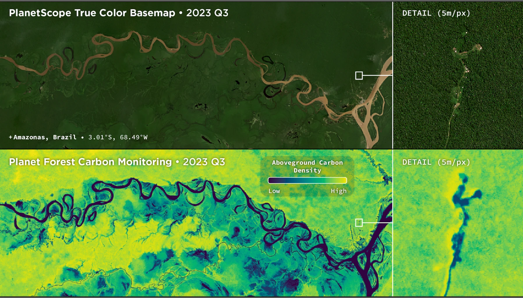
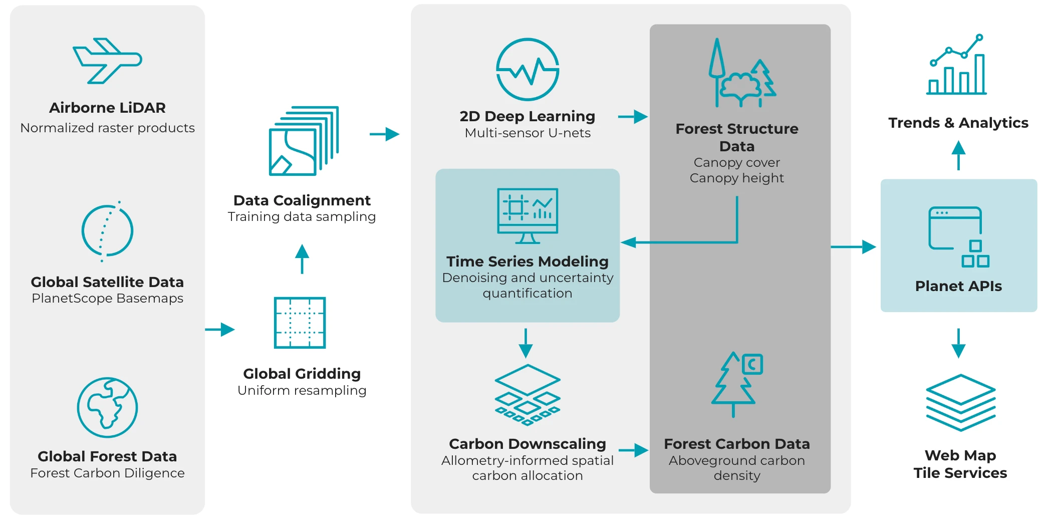
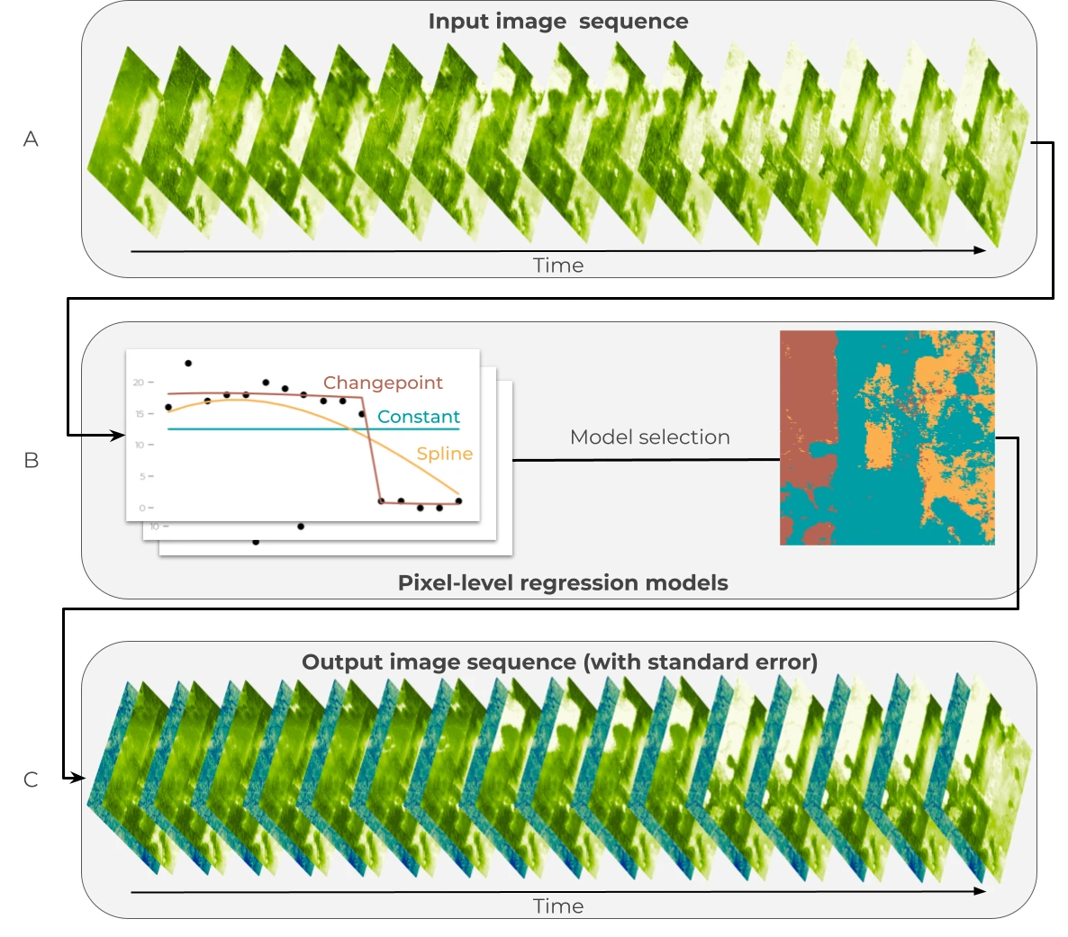
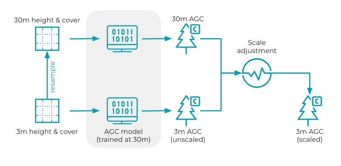
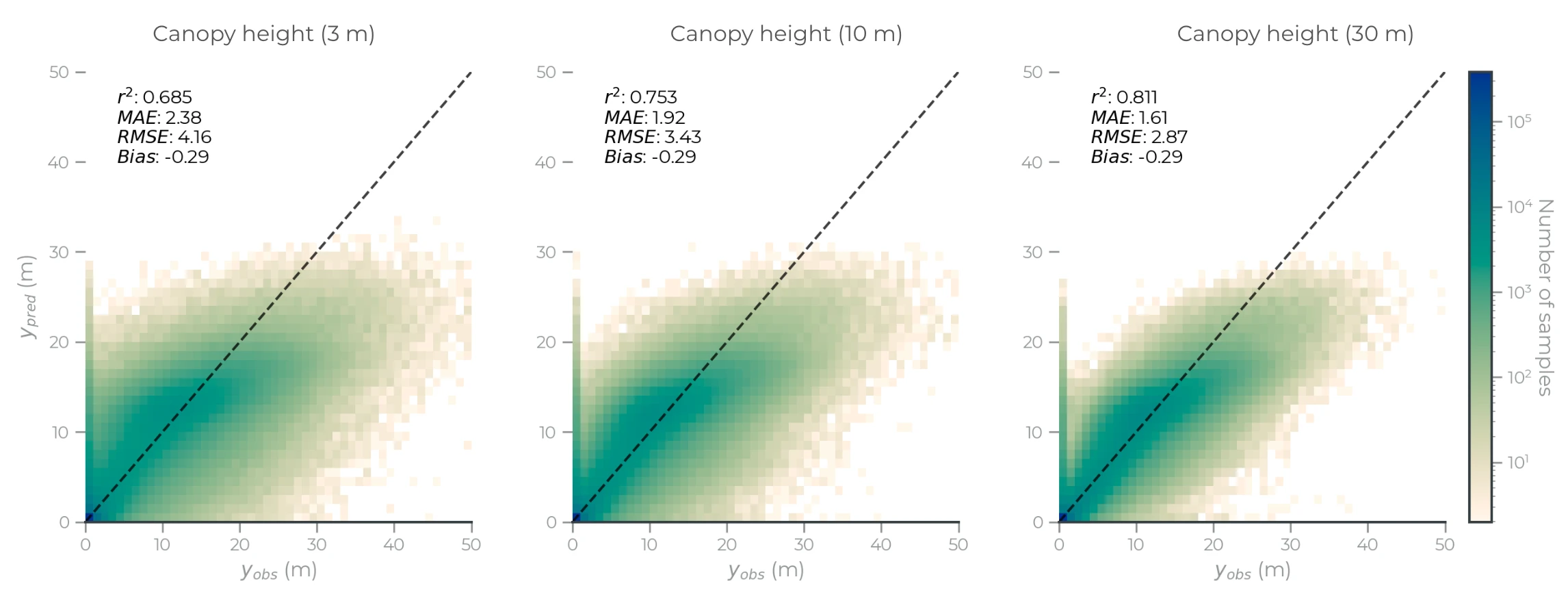
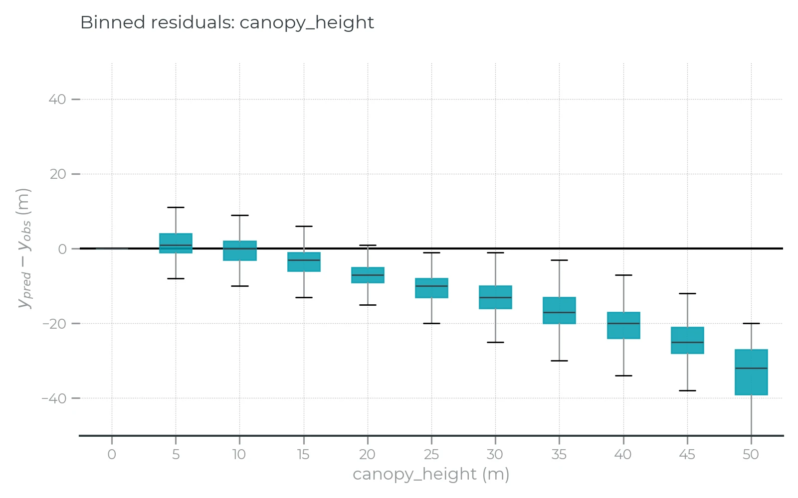
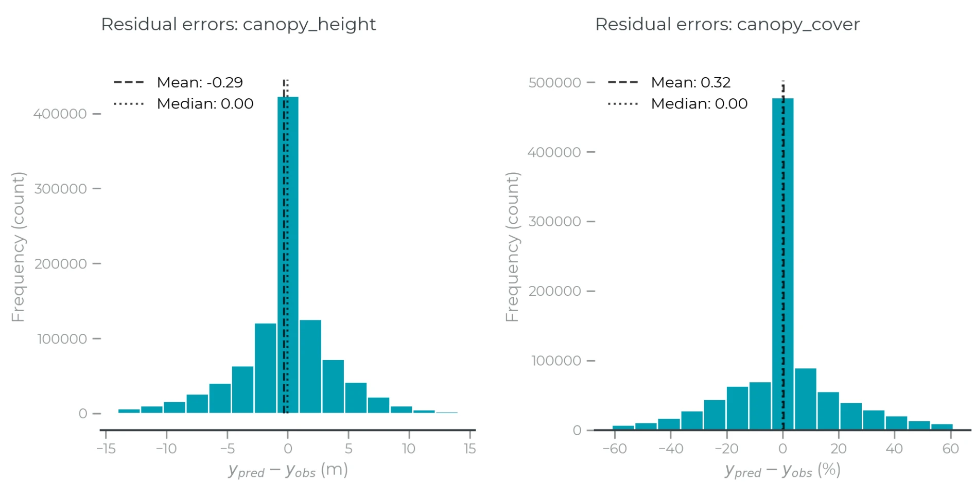

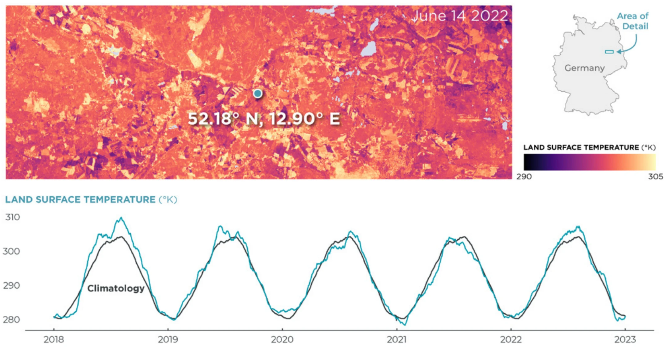
40° latitude: 274 to 292 observations per overpass time per year | | Overpass Time | 01:30 and 13:30 local solar time | | Geographical Coverage | Global | | Data Availability | 2018-01-01 - Present | | Satellites Used | AMSR-2, Sentinel-2 | | NRT latency (p90) | 24 hours | | Archive latency | Within 30 days after creating a subscription | *Table 2: LST 100 m product specification* | Data Resource | LST 100 m | | --------------------- | ------------------------------------------------------------------------------------------------------------------------------------------- | | Source ID | LST-AMSR2\_V1.0\_100 | | Version | 1.0 | | Unit | Kelvin | | Pixel Size | 0.00089° (±100x100 m) | | Temporal Resolution | 0° latitude: 205 to 228 observations per overpass time per year

40° latitude: 274 to 292 observations per overpass time per year | | Overpass Time | 01:30 and 13:30 local solar time | | Geographical Coverage | Global | | Data Availability | 2017-07-01 - Present | | Satellites Used | AMSR-2, Sentinel-2 | | NRT latency (p90) | 24 hours | | Archive latency | Within 30 days after creating a subscription | *Table 3: LST 1000 m product specification* | Data Resource | LST 1000 m | | --------------------- | ------------------------------------------------------------------------------------------------------------------------------------------- | | Source ID | LST-AMSR2\_V1.0\_1000 (2012 - present)

LST-AMSRE\_V1.0\_1000 (2002-2011) | | Version | 1.0 | | Unit | Kelvin | | Pixel Size | 0.00901° (±1000x1000 m) | | Temporal Resolution | 0° latitude: 205 to 228 observations per overpass time per year

40° latitude: 274 to 292 observations per overpass time per year | | Overpass Time | 01:30 and 13:30 local solar time | | Geographical Coverage | Global | | Data Availability | 2002-06-15 - Present

Data gap:
2011-10-04 to 2012-07-25 | | Satellites Used | AMSR-2, AMSR-E | | NRT latency (p90) | 24 hours | | Archive latency | Within 30 days after creating a subscription | ## Asset Properties Assets differ between field-based and tile-based data resources: * **LST 20 m (field-based)**: Each observation is delivered as a single-band asset with metadata embedded in the GeoTIFF. * **LST 100 m and LST 1000 m (tile-based)**: Each observation is delivered as a LST data asset (`*lst.tif`) with metadata provided in a separate quality flag asset (`*lst-qf.tif`). *Table 4: Asset properties of LST 20 m data resources* | Asset Name | Band Name | Unit | Type | Typical Range | No Data Value | Scale | Format | | ---------- | --------- | ------ | ------ | ------------- | ------------- | ----- | ------- | | lst | Band 1 | kelvin | UINT16 | 263-340 | 65535 | 0.01 | GeoTIFF | *Table 5: Asset properties of LST 100 m and LST 1000 m data resources* | Asset Name | Band Name | Unit | Type | Typical Range | No Data Value | Scale | Format | | ---------- | --------- | -------- | ------ | ------------- | ------------- | ----- | ------- | | lst | Band 1 | kelvin | UINT16 | 263 - 340 | 65535 | 0.01 | GeoTIFF | | lst | Band 2 | kelvin | UINT16 | 250 - 360 | 65535 | 0.01 | GeoTIFF | | lst-qf | Band 1 | unitless | UINT16 | NA | 0 | 1 | GeoTIFF | You can find below a Python code snippet that converts a temperature from Kelvin to Celsius and Fahrenheit: ``` def kelvin_to_celsius(kelvin): return kelvin - 273.15 def kelvin_to_fahrenheit(kelvin): celsius = kelvin - 273.15 return (celsius * 9/5) + 32 ``` ## Methodology ### Passive Microwaves and Downscaling Method The Ka band (±36.5 GHz) vertical polarized brightness temperature is used to derive LST because it is considered the most appropriate microwave frequency for temperature retrieval. This channel balances a reduced sensitivity to soil surface characteristics with a relatively high atmospheric transmissivity. It is shown that with a simple linear relationship, accurate values for LST can be obtained from this frequency [Holmes et al., 2009](https://doi.org/10.1029/2008JD010257). The downscaling patented technology ([US10643098](https://patentimages.storage.googleapis.com/1a/6f/1c/8cf51399ee7eaa/US10643098.pdf), [EP3469516B1](https://patentimages.storage.googleapis.com/f1/6c/0b/55cad50731d3e0/EP3469516B1.pdf)) aims to improve the resolution of sensor data, in this case, the brightness temperatures observed by passive microwave sensors. The technique redefines the exact geolocation and reconstructs the antenna footprints of each observation. It uses the abundance of overlaps between these footprints for downscaling at a target resolution. Based on the footprint center, microwave frequency, incidence angle, azimuth angle, and footprint size for a given intensity, footprints are created and disaggregated in equal interval ellipses using an internal gaussian distribution. Within the ellipse-shaped footprints, the center of the footprint contributes more to the observed values than the edges. Water bodies will have a fixed value and will be considered; thus, the land brightness temperature can be retrieved more accurately. This method elucidates the exact source of the signal of each observation point. The output of the downscaling method is brightness temperature for a given frequency at the target resolution. ### Enhancements Using Optical Data Land Surface Temperature is also highly variable in space, mainly due to soil properties, topography, agricultural practices, and land cover heterogeneity. Space-borne optical/thermal sensors can help retrieve high-resolution surface parameters. Several studies ([Lobell & Asner 2002](https://doi.org/10.2136/sssaj2002.7220), [Fensholt and Sandholt 2003](https://www.sciencedirect.com/science/article/abs/pii/S0034425703001895), [Sadeghi et al. 2017](https://doi.org/10.1016/j.rse.2017.05.041), [Yue et al. 2019](https://doi.org/10.1016/j.isprsjprs.2019.06.012)) found that soil and plant water content greatly influences the reflection in the shortwave infrared (SWIR) part of the spectrum. The SWIR, combined with the Near-Infrared (NIR) reflectance, which is affected by internal leaf structure and leaf dry matter content but not by water content, will enhance the LST retrieval from reflectances. We produce a daily NDSWIR composite using a backward Gaussian weighted distribution. This composite integrates into the downscaling framework by attributing the weight of a brightness temperature to each pixel within the footprint. The output format remains similar to that of the downscaling algorithm without NDSWIR input. The Sentinel-2 data is extracted from L2A - Bottom of the atmosphere (BOA) - reflectance in the [Sentinel-2 dataset documentation](https://docs.planet.com/data/public-data/copernicus/sentinel-2.md). ### Input Data *Table 6: List of inputs for Land Surface Temperature production* | Product | Description | | --------------------------------------------- | -------------------------------------------------------------------------------------------------------------------------------------------------------------------------------------------------------------------------------------------------------------------------------------------------------------------------------------------------------------------------------------------------------------------------------------------------------------------------------------------------------------------------------------------------------------------------- | | Brightness Temperature Ka band | AMSR-E and AMSR-2 Level-1B Radiometer Ka band Brightness Temperatures (downloaded from [JAXA G-portal](https://gportal.jaxa.jp/gpr/?lang=en) in HDF5 format). This Level-1B product provides calibrated estimates of geolocated brightness temperatures at 36.5 GHz with a footprint size of 7x12 km. Data has been available from July 2002 to October 2011 (AMSR-E) and from June 2012 (AMSR-2) up to now with a latency of 12 hours. Detailed information is available [here](https://gportal.jaxa.jp/gpr/assets/mng_upload/GCOM-W/AMSR2_Level1_Product_Format_EN.pdf). | | Brightness Temperature W band | AMSR-E and AMSR-2 Level-1B Radiometer W band Brightness Temperatures (downloaded from JAXA G-portal in HDF5 format). This Level-1B product provides calibrated estimates of geolocated brightness temperatures at 89 GHz with a footprint size of 3x5 km. Data has been available from July 2002 to October 2011 (AMSR-E) and from June 2012 (AMSR-2) up to now with a latency of 12 hours. Detailed information is available [here](https://gportal.jaxa.jp/gpr/assets/mng_upload/GCOM-W/AMSR2_Level1_Product_Format_EN.pdf). | | Reflectances SWIR and NIR (for LST 20m/100 m) | Sentinel-2 Level-2A reflectance [data](https://docs.planet.com/data/public-data/copernicus/sentinel-2.md) for two bands: SWIR (shortwave infrared around 1610 nm) and NIR (near infrared around 842 nm). | | Digital Elevation Model | Digital elevation model (DEM) static map based on the Copernicus DEM GLO-90 product covering the full global landmass of the time frame of data acquisition (2011-2015). Detailed information is available in the link. | | Land Cover Map | Custom global land classification including permanent water bodies based on the Copernicus Global Surface Water Bodies product from PROBA-V. Detailed information is available [here](https://land.copernicus.eu/global/) | ## Data Quality ### Validation We have evaluated our LST products by comparing them to carefully ground data stations and other remotely sensed LST data across various land cover types and climates regions. You can read more about the results in [this white paper](https://planet.widen.net/s/j9rl92dgpq). Planet's 1 km LST product was validated over 114 locations from 2013-01-01 to 2022-12-31. We used an established network of in-situ stations from the United States Climate Reference Network (USCRN) and remotely sensed LST derived from MODIS AQUA. The Planet 1 km LST, MODIS AQUA 1 km LST and USCRN surface temperature were intercompared at 1:30 and 13:30, separately. The surface temperature at USCRN stations is measured over grassy or low vegetation (< 10 cm) surfaces and the stations cover many climatic and landscape conditions. ![](/data/planetary-variables/land-surface-temperature/lst_validation_ts.webp) *Figure 2: Time series of nighttime (upper figures) and daytime (lower figures) land surface temperature for the in-situ observations from the United States Climate Reference Network (USCRN), MODIS and Planet’s 1 km products between 2013 and 2022 at the USCRN station Yuma (32.835, -114.1884), AZ, U.S. The scatterplots on the right compare single observations from MODIS’ and Planet’s LST against the in-situ observations for nighttime (Mean Absolute error (MAE) for MODIS: 1.28; MAE for Planet 1 km: 1.83) and daytime (MAE for MODIS: 3.40; MAE for Planet 1 km: 2.96).* In the validation report, a spatial comparison of the Planet 100m LST against Landsat LST. The revisit time of Landsat is low with one observation every 8 days at best, since thermal-based LST is sensitive to cloud cover. The overpass time of Landsat is between 10:00 and 10:25 while Planet LST daytime is at 13:30. Due to the mismatch in observation time, the focus on the analysis is on the relative spatial variability, rather than the absolute comparison. ![](/data/planetary-variables/land-surface-temperature/lst_validation.webp) *Figure 3: Spatial comparison of 100 m LST compared to Landsat LST. The scatterplot on the left presents a comparison for agricultural fields on single day between Landsat and Planet LST, the right figures are the maps of the day compared. The area of interest are (top) Nordrhein Westfalen, near Düsseldorf in Germany and (bottom) southwest of Imperial, Nebraska, in the United States.* ### Metadata #### LST 20 m Metadata embedded in the GeoTIFF contains information about the quality of the observation. For example: | Field | Type | Description | Example | | ------------------- | ----------------- | --------------------------------------------------------------------------- | -------------------------------------------- | | `PRODUCT_VERSION` | String | Version identifier for the product specification | `v1` | | `SOFTWARE_VERSION` | String | Version of the fbsl software that generated the output | `0.4.1` | | `INPUT_ASSETS` | String | Comma-separated list of input data sources used | `NDSWIR_STATS,NDSWIR_RASTER,KA_V_DESC_STATS` | | `LAST_NDSWIR_DATE` | String (ISO date) | Date of the last NDSWIR (Sentinel-2) observation with full coverage | `2024-01-19` | | `LAST_NDSWIR_COV` | String (fraction) | Coverage fraction of the last NDSWIR observation used | `0.85` (= 85% coverage) | | `QUALITY` | String | Overall quality assessment: `HIGH` if valid coverage > 80%, otherwise `LOW` | `HIGH` or `LOW` | | `INVALID_RANGE_COV` | String (fraction) | Fraction of pixels outside valid LST range (250-340 K) | `0.02` (= 2% invalid) | #### LST 100 m and LST 1000 m Quality flag assets (`*lst-qf.tif`) provide metadata for each pixel using bitwise flags. Critical flags indicate unreliable data, with corresponding pixels in band 1 of the LST asset (`*lst.tif`) set to the no data value. The replaced LST value can be found in band 2 of the LST asset. Non-critical flags indicate that the data can be used with caution, taking into account the flag description. Critical and non-critical flags are described in the tables below. For more information on how to access the quality flag asset, check out [subscribing to Planetary Variables](https://docs.planet.com/develop/apis/subscriptions/sources.md). *Table 7: Non-critical flags* | Bit | Flag layer | Description | | --- | ----------------------------- | ------------------------------------------------------------------------------------------------------------------- | | 4 | Possible severe precipitation | Part of the footprints touch an area flagged as severe precipitation. | | 7 | Possible frozen soil | The surface may be frozen. These are pixels with a surface temperature between 263.15 K (-10°C) and 273.15 K (0°C). | *Table 8: Critical flags* | Bit | Flag layer | Description | | --- | -------------------- | ----------------------------------------------------------------------------------------------------------------------------------------------------------------------------------------------------------------------- | | 8 | Frozen soil | The surface is considered frozen. Pixels with a temperature below 263.15 K (-10°C). | | 9 | Severe precipitation | Severe precipitation is detected. | | 11 | No overpass | The satellite did not pass over. | | 13 | Instrumental flaws | Unrealistic values due to instrumental flaws. If the brightness temperature at 36.5 GHz V produces values either over 400K or under 0.9 \* the water temperature, the data is considered as unrealistic and is removed. | | 14 | Out of valid range | Land Surface Temperature values are outside the valid range, meaning under 250 K or above 340 K. | | 15 | Open water | Land Surface Temperature is not defined over water (retrieved from a land cover map). This data is filtered out during the processing of the raw satellite data. | Here is a Python script to convert a quality flag pixel value into a list of corresponding quality flags. Note that one pixel may have multiple flags applied to it. ``` # lst_quality_flags.py import argparse LST_QUALITY_FLAGS = { 4: "Possible severe precipitation", 7: "Possible frozen soil", 8: "Frozen Soil (critical flag)", 9: "Severe precipitation (critical flag)", 11: "No overpass (critical flag)", 13: "Instrumental flaws (critical flag)", 14: "Out of valid range (critical flag)", 15: "Open water (critical flag)", } def convert_to_quality_flags(decimal_value: int) -> list[str]: binary_string = format(decimal_value, "016b") reversed_binary_string = binary_string[::-1] return [ f"{i}. {LST_QUALITY_FLAGS.get(i, 'Unused flag')}" for i, bit in enumerate(reversed_binary_string, start=1) if bit == "1" ] if __name__ == "__main__": parser = argparse.ArgumentParser(description="Convert a decimal value to quality flags.") parser.add_argument("decimal_value", type=int, help="The decimal value to convert.") args = parser.parse_args() flags = convert_to_quality_flags(args.decimal_value) print(*flags, sep="\n") ``` that you can call as follows, using value `8512` as example: ``` > python lst_quality_flags.py 8512 7. Possible frozen Soil 9. Severe precipitation (critical flag) 14. Out of valid range (critical flag) ``` ### Other Limitations The following are some key limitations that we have not flagged: * Data should be considered unreliable over sloped terrain that is over 20 degrees. The microwave signal can be distorted by the angle of the slope, causing changes in the observed brightness temperature. This distortion leads to inaccuracies in the Land Surface Temperature estimates because the algorithms assume a flat surface. * Dynamic water bodies may cause unrealistic Land Surface Temperature estimates. Water bodies influence the microwave observations and without proper mitigation they could result in unrealistic retrievals. * Persistent cloud cover in highly dynamic landscape can decrease the downscaling method accuracy due to the optical observations by Sentinel-2 that are used for the LST 100 m products. * False cloud/shadow detections may occur if surface conditions change very rapidly, during prolonged cloudiness, or over AOIs with significant terrain and shadowing. Significant effort has gone into developing automated techniques to differentiate between actual change and atmospheric contamination, but there may still be false detections. ## Frequently Asked Questions ### What do you actually measure? We measure the skin temperature of the first thing in the line of sight of the satellite. This can be a roof, a tarmac road, a tree or crop canopy, bare soil or a mixture of land cover types. ### Do you measure the soil temperature? No, we measure the temperature at the actual surface, the skin temperature. However, this is highly correlated to the soil temperature ### How accurate is the data? Accuracy of the data is comparable with existing Land Surface Products products such as MODIS but we provide higher resolution and more valid data points. Check the [validation white paper](https://planet.widen.net/s/j9rl92dgpq) for actual numbers. ### How about frost use cases? At the moment our LST should not be relied upon for below freezing point temperatures. Data below 263 kelvin (-10°C) is filtered out and data below 273 kelvin (0°C) should be treated with care. ### What type of satellites are used to determine Land Surface Temperature? Most of the signal is from the passive microwave satellites (AMSR-2 and AMSR-E) and Sentinel-2 optical data is used to enhance to 100m. The passive microwave satellites measure microwave signals that are naturally radiating from the Earth’s surface. This enables observations to be acquired during cloudy conditions, because of the physical properties of waves transmitted in this spectrum’s range. ### What is the difference between the LST 100 m and 1000 m products? Our LST 1000 m product is based on our patented disaggregation method where we make optimum use of the overlapping satellite footprints to refine the resolution from 36 km to 1 km. The LST 100 m product also uses the NIR and SWIR band from Sentinel-2 to add more spatial constraints to our disaggregation method. ### When is the data observed? Currently, Planet uses the daytime and nighttime observations during the ascending and descending orbits, respectively. For AMSRE and AMSR2 this corresponds to 01:30 and 13:30 local solar time. ### What is the coverage of the data in terms of observations? Each of the microwave satellites are on a sun-synchronous orbit. Using both orbit directions (ascending and descending) we can retrieve LST up to twice a day. The observation coverage is less frequent around the equator, where the Earth is ‘widest’ around its longitude belt, and more frequent at high latitudes, where the longitude belts are less wide. One can expect between 180 (at equator) and 365 (above 50°N) daytime and nighttime measurements per year, depending on the geographical location. ![](/data/planetary-variables/land-surface-temperature/lst_global.gif) *Land Surface Temperature animation of the 16-day AMSR2 cycle from 2024-06-02 to 2024-06-17* ### What about cloud cover? The microwave part of the observations is not hindered by cloud cover. However, for downscaling to 100 m, we rely on near-infrared and shortwave infrared data that are sensitive to cloud cover. As such, there will be regions that will show artifacts in the 100 m data due to long periods with clouds. For all regions with > 70% cloud cover data should only be delivered to clients after a manual inspection (100 m only). This also means that the 100 m is less suitable for monitoring high temporal frequency changes (at the small scale) in cloudy regions. ### Can we measure water surface temperature? No. The water bodies are removed from the signal because they may cause unrealistic Land Surface Temperature estimates. Water bodies influence the microwave observations and without proper mitigation they could result in unrealistic retrievals. ## Release notes ### Jun 1, 2025 - LST 20 m v1.0 New Features * Increased spatial resolution (25x) * Field-based processing * Metadata as raster-level tags in each geotiff (1-band raster delivered per observation) --- Copy for LLM[View as Markdown](https://docs.planet.com/data/planetary-variables/soil-water-content/) # Soil Water Content ![Header Thumbnail](/data/planetary-variables/soil-water-content/swc_thumbnail.webp) Soil water content is the amount of water between the soil surface and the groundwater level in the unsaturated zone. This ratio of water volume to soil volume is crucial for understanding soil health, hydrological processes, and drought conditions. The Planet Soil Water Content (SWC) product offers near-daily measurements with spatial resolutions of 20 m, 100 m, and 1000 m. Based on passive microwave observations, our data is consistent across time and space, strongly correlating with ground data and accurately reflecting weather patterns. This makes it a cost-effective and low-effort alternative to physical soil water content sensors. ## Use Cases **Agriculture** - You can use SWC data to develop models that assess field conditions, enabling more informed decisions about irrigation and field operations. The data is also used to make yield and crop quality predictions at both regional and field scales. **Drought Monitoring** - Tracking conditions over years and decades, SWC data provides a baseline understanding of normal and abnormal conditions for any given region. Leading reinsurers and brokers use the data in more than 20 countries to help protect farmers from drought impacts. **Water Resource Management** - Near real-time SWC data aids in monitoring complex water systems by offering insights into water demand and storage capacity. With over two decades of archive data, water resource managers can track droughts, measure soil saturation, and assess intervention effects. **Natural Disaster Risk Assessment** - Models incorporating vegetation, weather, and SWC data offer detailed insights into risks for wildfires, floods, and other natural disasters. The data also helps evaluate the impact of ecosystem restoration projects. Compared to in-situ sensors, SWC data provides a cost-effective and less labor-intensive method for risk assessment and remediation tracking. ## API Access Information | API | Available | Notes | | ----------------- | --------- | ----- | | Data API | ❌ | | | Orders API | ❌ | | | Subscriptions API | ✅ | | | Analytics API | ❌ | | | Basemaps API | ❌ | | ### Subscriptions Access #### Soil Water Content 20 m warning SWC 20 m is a beta product. This means the product is still under active development and may undergo changes to its methodology, accuracy, or availability. While the data is available for use, users should be aware that the product may have limitations or may be updated based on ongoing validation and feedback. Loading... The area of interest for SWC 20 m should correspond to a single agricultural field. If the AOI of a subscription includes multiple fields, whether they contain different crops or the same crop managed differently, the resulting SWC data will not accurately reflect conditions within any specific field. Similarly, if the AOI of a subscription includes non-agricultural areas, such as urban areas or water bodies, the resulting SWC data will not accurately reflect conditions within the AOI. #### Soil Water Content 100 m Loading... #### Soil Water Content 1000 m Loading... For more information on the Subscriptions API and code samples, see the [API documentation](https://docs.planet.com/develop/apis/subscriptions/sources.md#planetary-variable-and-analysis-ready-source-types). ## Additional Resources [🎓Planet University](https://university.planet.com/intro-to-soil-water-content) [Learn the SWC basics with this introduction course.](https://university.planet.com/intro-to-soil-water-content) [💡Blog posts](https://www.planet.com/pulse/tag/soil-water-content/) [Read the latest SWC news and stories.](https://www.planet.com/pulse/tag/soil-water-content/) [📖Subscriptions API](https://docs.planet.com/develop/apis/subscriptions.md) [Get started with the Subscriptions API.](https://docs.planet.com/develop/apis/subscriptions.md) [📓Jupyter Notebooks](https://github.com/planetlabs/notebooks/blob/master/jupyter-notebooks/api_guides/subscriptions_api/soil_water_content_gcp_delivery.ipynb) [Access SWC and create visualizations with this tutorial.](https://github.com/planetlabs/notebooks/blob/master/jupyter-notebooks/api_guides/subscriptions_api/soil_water_content_gcp_delivery.ipynb) [📖EvalScripts](https://custom-scripts.sentinel-hub.com/custom-scripts/planetary-variables/soil-water-content/) [Visualize SWC and extract insights with EvalScripts.](https://custom-scripts.sentinel-hub.com/custom-scripts/planetary-variables/soil-water-content/) --- Copy for LLM[View as Markdown](https://docs.planet.com/data/planetary-variables/soil-water-content/products/) # Products ## Soil Water Content 20 m Loading... ## Soil Water Content 100 m Loading... ## Soil Water Content 1000 m Loading... --- Copy for LLM[View as Markdown](https://docs.planet.com/data/planetary-variables/soil-water-content/sandbox/) # Soil Water Content Sandbox Data This Planet Sandbox Data collection for Soil Water Content provides sample data over specific areas and times of interest. The data is available to paid and trial accounts that include processing units and is available under the CC-BY-NC license. Learn more about [Planet Sandbox Data](https://docs.planet.com/data/planet-sandbox-data.md). ## Data Collections Metadata | Source ID | Collection Name | Collection ID | Time Range | | ---------------------- | -------------------------------- | ----------------------------------------- | ----------------------- | | SWC-SMAP-L\_V5.0\_1000 | Planet Sandbox Data - PV SWC 1km | BYOC-858254ae-0f29-4152-ac53-449efa00bbb0 | 2015-04-01 - 2023-12-31 | ## Planet Sandbox Data Areas This collection includes 17 sandbox regions. Download the GeoJSON file below the map for exact polygon boundaries. View all 17 regions | Location | Area (km²) | Time Range | Center (lat, lon) | | ------------------------------------------------- | ---------- | ----------------------- | ----------------- | | Arizona, United States | 579 | 2015-04-01 – 2023-12-31 | 32.86, -111.85 | | Alberta, Canada | 580 | 2015-04-01 – 2023-12-31 | 50.15, -111.78 | | Iowa, United States | 2320 | 2015-04-01 – 2023-12-31 | 41.19, -93.81 | | Goiás, Central-West Region, Brazil | 575 | 2015-04-01 – 2023-12-31 | -16.52, -48.83 | | Autonomous Community of the Basque Country, Spain | 576 | 2015-04-01 – 2023-12-31 | 42.81, -2.51 | | Nouvelle-Aquitaine, Metropolitan France, France | 2304 | 2015-04-01 – 2023-12-31 | 44.84, -0.52 | | Flevoland, Netherlands | 579 | 2015-04-01 – 2023-12-31 | 52.50, 5.71 | | Groningen, Netherlands | 576 | 2015-04-01 – 2023-12-31 | 53.15, 6.37 | | Emilia-Romagna, Italy | 576 | 2015-04-01 – 2023-12-31 | 44.97, 9.81 | | Epirus and Western Macedonia, Greece | 576 | 2015-04-01 – 2023-12-31 | 40.65, 21.76 | | Attica, Greece | 576 | 2015-04-01 – 2023-12-31 | 38.02, 23.92 | | Kitui County, Kenya | 578 | 2015-04-01 – 2023-12-31 | -1.34, 37.85 | | Al Jawf Region, Saudi Arabia | 576 | 2015-04-01 – 2023-12-31 | 30.05, 38.42 | | Haryana, India | 578 | 2015-04-01 – 2023-12-31 | 27.86, 77.36 | | Thái Bình Province, Vietnam | 576 | 2015-04-01 – 2023-12-31 | 20.51, 106.30 | | Guizhou, Tongren, China | 575 | 2015-04-01 – 2023-12-31 | 28.09, 109.21 | | New South Wales, Australia | 581 | 2015-04-01 – 2023-12-31 | -34.52, 146.13 | [Download GeoJSON](https://docs.planet.com/data/planetary-variables/soil-water-content/polygons.geojson) --- Copy for LLM[View as Markdown](https://docs.planet.com/data/planetary-variables/soil-water-content/techspec/) # Technical Specification ## Overview Soil water content (SWC) is an essential component of the hydrologic cycle. Also known as soil moisture, it refers to the water between the soil surface and the groundwater level in the unsaturated zone. This water is replenished by precipitation, irrigation, or capillary rise from deeper layers, and depleted by percolation, soil evaporation, and plant transpiration. The Planet Soil Water Content product is based on the microwave radiation naturally emitted by the Earth. This passive microwave radiation is related to the water content in the soil and provides a direct measurement of water in the top layer of the soil. It is not sensitive to cloud cover and, therefore, allows for consistent, frequent, and global coverage. The Planet patented algorithm enhances the spatial resolution of the passive microwave observations and the physical-based Land Parameter Retrieval Model retrieves the soil water content. Optical imagery from Sentinel-2 is used to further improve the spatial resolution. Planet provides SWC data at 20, 100, and 1000 meter resolutions. With an archive spanning over 20 years, the data is consistent across time and space, boasting a strong correlation with ground data and accurately reflecting weather patterns. It is a cost-effective and low-effort alternative for measuring soil water content with physical sensors, making it suitable for many use cases like agriculture, water management, and insurance. ![](/data/planetary-variables/soil-water-content/swc_time_series.webp) *Figure 1: Measurements of SWC near Ahlen, in North Rhine-Westphalia, Germany. The measurements of SWC of a single point are plotted over 5 years with the baseline climatology, showing how soil water content levels compare to the expected average for the area.* ## Product Specifications warning SWC 20 m is a beta product. This means the product is still under active development and may undergo changes to its methodology, accuracy, or availability. While the data is available for use, users should be aware that the product may have limitations or may be updated based on ongoing validation and feedback. *Table 1: SWC 20 m product specification* | Data Resource | SWC 20 m | | --------------------- | ------------------------------------------------------------------------------------------------------------------------------------ | | Source ID | SWC-field\_V1.0\_20 | | Satellites Used | AMSR-2, AMSR-E, SMAP, Sentinel-2 | | Band | L, C and X-band | | Version | 1.0 | | Unit | m³/m³ | | Sensing Depth | \~5 cm | | Pixel Size | 20x20 m | | Temporal Resolution | 267-364 observations/year | | Overpass Time | 06:00 local solar time | | Geographical Coverage | Global | | Data Availability | 2018-01-01 - Present
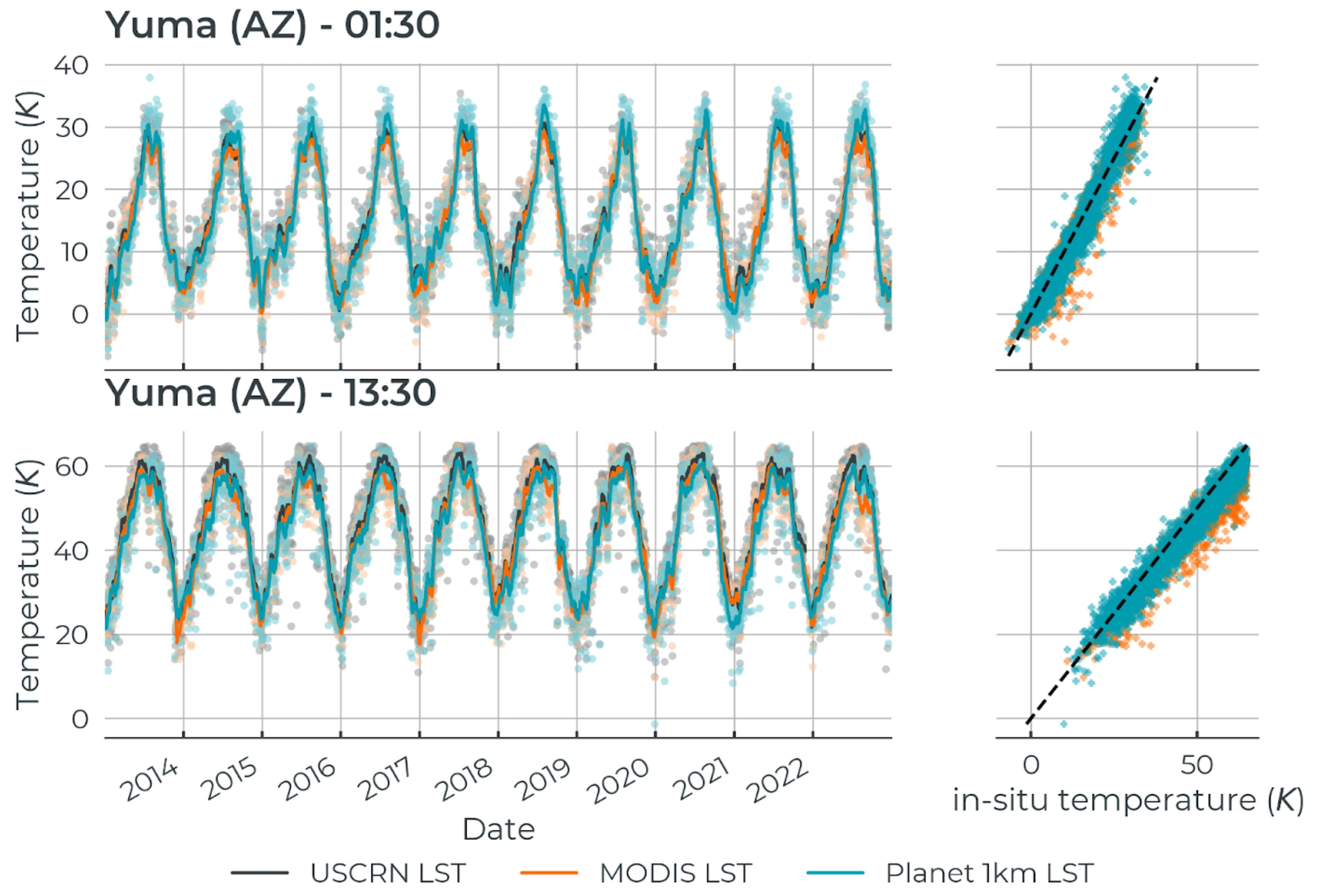
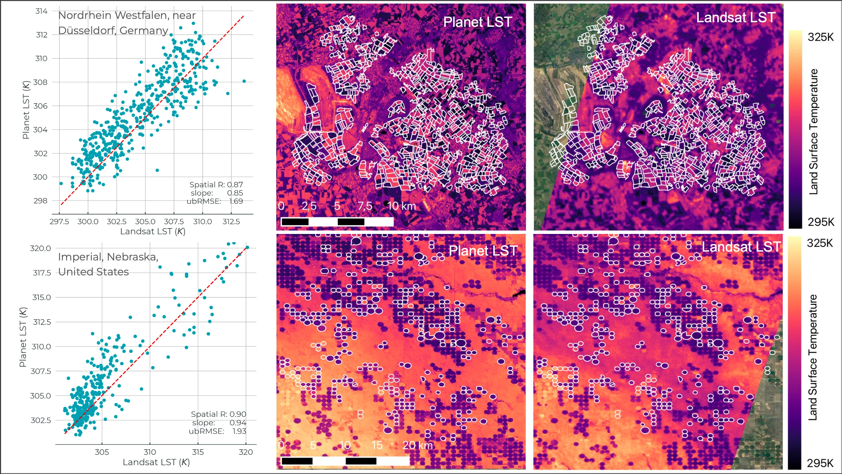
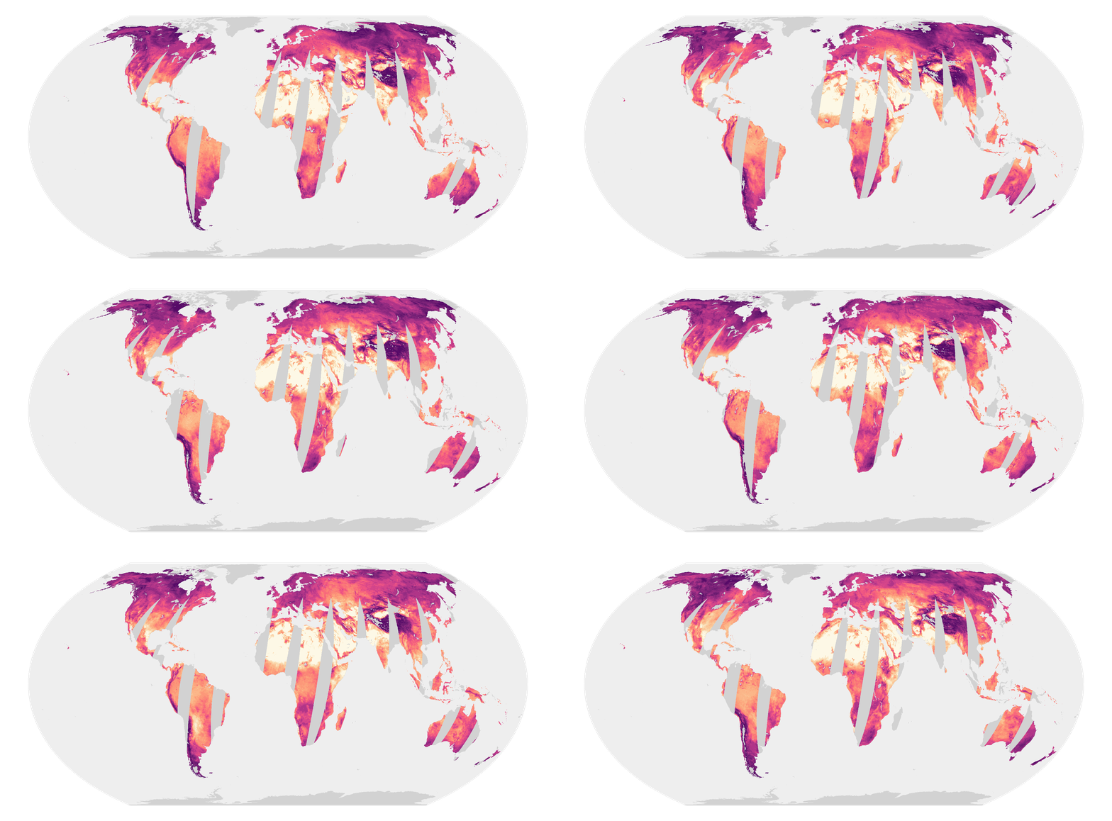

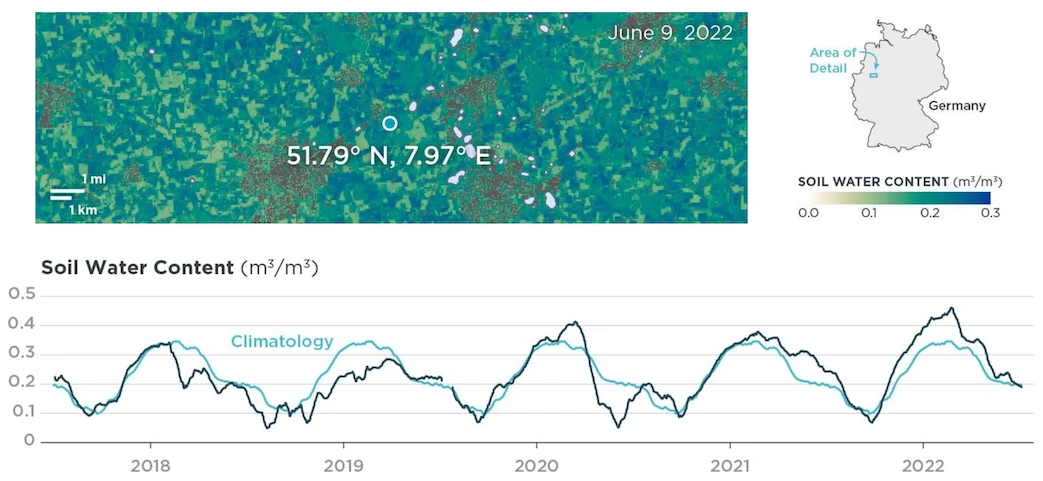
Data Gaps:
2019-06-19 to 2019-07-24
2022-08-05 to 2022-09-24
2022-11-16 to 2022-11-18 | *Table 2: SWC 100 m product specification* | Data Resource | SWC 100 m L band | SWC 100 m C band | SWC 100 m X band | | --------------------- | ------------------------------------------------------------------------------------------------------------------------------------ | ------------------------------------------------------------------------------------------------------- | ------------------------------------------------------------------------------------------------------- | | Source ID | SWC-SMAP-L\_V2.0\_100 | SWC-AMSR2-C\_V2.0\_100 | SWC-AMSR2-X\_V2.0\_100 | | Satellites Used | AMSR-2, SMAP, Sentinel-2 | AMSR-2, Sentinel-2 | AMSR-2, Sentinel-2 | | Band | L band | C band | X band | | Version | 2.0 | 2.0 | 2.0 | | Unit | m³/m³ | m³/m³ | m³/m³ | | Sensing Depth | \~5 cm | \~2 cm | \~1 cm | | Pixel Size | 100x100 m | 100x100 m | 100x100 m | | Temporal Resolution | 0° latitude: 137 to 183 observations per year

40° latitude: 183 to 228 observations per year | 0° latitude: 205 to 228 observations per year

40° latitude: 274 to 292 observations per year | 0° latitude: 205 to 228 observations per year

40° latitude: 274 to 292 observations per year | | Overpass Time | 06:00 local solar time | 01:30 local solar time | 01:30 local solar time | | Geographical Coverage | Global | Global | Global | | Data Availability | 2017-07-01 - Present

Data Gaps:
2019-06-19 to 2019-07-24
2022-08-05 to 2022-09-24
2022-11-16 to 2022-11-18 | 2017-07-01 - Present | 2017-07-01 - Present | | NRT latency (p90) | 72 hours | 48 hours | 48 hours | | Archive latency | Within 30 days after creating a subscription | Within 30 days after creating a subscription | Within 30 days after creating a subscription | *Table 3: SWC 1000 m product specification* | Data Resource | SWC 1000 m L band | SWC 1000 m C band | SWC 1000 m X band | | --------------------- | ------------------------------------------------------------------------------------------------------------------------------------ | ------------------------------------------------------------------------------------------------------- | --------------------------------------------------------------------------------------------------- | | Source ID | SWC-SMAP-L\_V5.0\_1000 | SWC-AMSR2-C\_V5.0\_1000
(2012 - present)

SWC-AMSRE-C\_V5.0\_1000
(2002 - 2011) | SWC-AMSR2-X\_V5.0\_1000
(2012 - present)

SWC-AMSRE-X\_V5.0\_1000
(2002 - 2011) | | Version | 5.0 | 5.0 | 5.0 | | Unit | m³/m³ | m³/m³ | m³/m³ | | Sensing Depth | \~5 cm | \~2 cm | \~1 cm | | Pixel Size | 1000x1000 m | 1000x1000 m | 1000x1000 m | | Temporal Resolution | 0° latitude: 137 to 183 observations per year

40° latitude: 183 to 228 observations per year | 0° latitude: 205 to 228 observations per year

40° latitude: 274 to 292 observations per year | 0° latitude: 205 to 228 obs/year

40° latitude: 274 to 292 obs/year | | Overpass Time | 06:00 local solar time | 01:30 local solar time | 01:30 local solar time | | Geographical Coverage | Global | Global | Global | | Data Availability | 2015-04-01 - Present

Data Gaps:
2019-06-19 to 2019-07-24
2022-08-05 to 2022-09-24
2022-11-16 to 2022-11-18 | 2002-06-15 - Present

Data gap:
2011-10-04 to 2012-07-25 | 2002-06-15 - Present

Data gap:
2011-10-04 to 2012-07-25 | | Satellites Used | AMSR-2, SMAP | AMSR-E, AMSR-2 | AMSR-E, AMSR-2 | | NRT latency (p90) | 72 hours | 24 hours | 24 hours | | Archive latency | Within 30 days after creating a subscription | Within 30 days after creating a subscription | Within 30 days after creating a subscription | The sensing depth described in the table is an estimation of the average condition. Several studies (For example, [Schmugge et al., 1986](https://ieeexplore.ieee.org/abstract/document/4072415); [Wang et al., 1987](https://ieeexplore.ieee.org/document/4072692); [Owe et al., 1998](https://agupubs.onlinelibrary.wiley.com/doi/abs/10.1029/98WR01469)) have shown that microwave-based soil water content penetration depth depends on the soil water content conditions and frequency. At 1.41 GHz the penetration depth varies from approximately 10 cm to 1 m for soil conditions ranging from saturated to dry, whereas at 10.7 GHz the penetration depth varies from less than a few mm to a little over 2 cm for similar conditions. Thus, the drier the soil, the deeper the sampling depth. ## Asset Properties Assets differ between field-based and tile-based data resources: * **SWC 20 m (field-based)**: Each observation is delivered as a single-band asset with metadata embedded in the GeoTIFF. * **SWC 100 m and SWC 1000 m (tile-based)**: Each observation is delivered as a SWC data asset (`*swc.tif`) with metadata provided in a separate quality flag asset (`*swc-qf.tif`). *Table 4: Asset properties of SWC 20 m data resources* | Asset Name | Band Name | Unit | Type | Typical Range | No Data Value | Scale | Format | | ---------- | --------- | ----- | ------ | ------------- | ------------- | ----- | ------- | | swc | Band 1 | m3/m3 | UINT16 | 0 - 1 | 65535 | 0.001 | GeoTIFF | *Table 5: Asset properties of SWC 100 m and SWC 1000 m data resources* | Asset Name | Band Name | Unit | Type | Typical Range | No Data Value | Scale | Format | | ---------- | --------- | -------- | ------ | ------------- | ------------- | ----- | ------- | | swc | Band 1 | m3/m3 | UINT16 | 0 - 1 | 65535 | 0.001 | GeoTIFF | | swc | Band 2 | m3/m3 | UINT16 | 0 - 1 | 65535 | 0.001 | GeoTIFF | | swc-qf | Band 1 | unitless | UINT16 | NA | 0 | 1 | GeoTIFF | ## Methodology ### Passive Microwaves and Downscaling Method The Planet Soil Water Content data is derived from satellite sensors that measure passive microwave radiation. Passive microwave technology detects natural microwave emissions from the Earth's surface, which are sensitive to soil water content. Using a patented algorithm ([US10643098](https://patentimages.storage.googleapis.com/1a/6f/1c/8cf51399ee7eaa/US10643098.pdf), [EP3469516B1](https://patentimages.storage.googleapis.com/f1/6c/0b/55cad50731d3e0/EP3469516B1.pdf)), we combine and downscale observations from multiple satellite constellation to a spatial resolution of 1000 m. We create footprints based on the footprint center, microwave frequency, incidence angle, azimuth angle, and footprint size, and then disaggregate them into equal interval ellipses using an internal Gaussian distribution. Within these ellipse-shaped footprints, the center contributes more to the observed values than the edges. By using fixed values for water bodies and filtering out influences such as radio frequency interference (RFI), we ensure accurate brightness temperatures. ### Enhancements Using Optical Data The microwave observations are further downscaled to a spatial resolution of 100 m based on the Normalized Difference Shortwave Infrared (NDSWIR) index. This index is constructed from Near-Infrared (NIR) and Shortwave Infrared (SWIR) bands of Sentinel-2, namely B08 (842 nm) and B11 (1610 nm). Several studies ([Lobell & Asner 2002](https://doi.org/10.2136/sssaj2002.7220), [Fensholt and Sandholt 2003](https://www.sciencedirect.com/science/article/abs/pii/S0034425703001895), [Sadeghi et al. 2017](https://doi.org/10.1016/j.rse.2017.05.041), [Yue et al. 2019](https://doi.org/10.1016/j.isprsjprs.2019.06.012)) found that soil and plant water content significantly affect the reflection in the SWIR part of the spectrum. The NIR reflectance is influenced by the internal structure and dry matter content of leaves, but not by water content. By combining SWIR, which responds to water content, with NIR reflectance, we can more accurately retrieve water content from the reflectance data ([Gao 1996](https://doi.org/10.1016/S0034-4257\(96\)00067-3), [Ceccato et al. 2001](https://doi.org/10.1016/S0034-4257\(01\)00191-2)). Planet produces a daily NDSWIR composite using a backward Gaussian weighted distribution. This composite integrates into the downscaling framework by attributing the weight of a brightness temperature to each pixel within the footprint. The output format remains similar to that of the downscaling algorithm without NDSWIR input. The Sentinel-2 data is extracted from L2A - Bottom of the atmosphere (BOA) - reflectance in the [Sentinel-2 dataset documentation](https://docs.planet.com/data/public-data/copernicus/sentinel-2.md). ### Physical-Based Land Parameter Retrieval Model The downscaled high resolution microwave observations are converted to soil water content using the physical-based Land Parameter Retrieval Model (LPRM) ([Owe et al. 2001](https://ieeexplore.ieee.org/abstract/document/942542); [Owe et al. 2008](https://agupubs.onlinelibrary.wiley.com/doi/full/10.1029/2007JF000769); [De Jeu et al. 2014](https://www.sciencedirect.com/science/article/abs/pii/S0022169414001139), [Van der Schalie et al., 2018](https://www.mdpi.com/2072-4292/10/1/107), [Van der Schalie et al., 2018](https://www.mdpi.com/2072-4292/13/13/2480)). The basis for the retrieval relies on the fact that thermal radiation in the microwave region is emitted by all natural surfaces as a function of temperature. The propagation of microwaves through the soil is then dependent on the soil dielectric constant, which has an almost linear relationship with soil water content. Microwave technology is the only remote sensing method that measures a direct response to the absolute amount of water in the soil, with a sensing depth ranging from millimeters for 37 GHz to tens of cm for 1.4 GHz. Vegetation also contributes to the microwave signal by absorbing, reflecting, and emitting radiation. LPRM solves the radiative transfer equation at different frequencies and polarizations to retrieve soil water content and is currently the baseline algorithm for the ESA Climate Change Initiative (CCI) soil moisture products ([Scanlon et al., 2021](https://esa-soilmoisture-cci.org/sites/default/files/documents/public/CCI%20SM%20v06.1%20documentation/ESA_CCI_SM_RD_D2.1_v2_ATBD_v06.1_issue_1.1.pdf)). ### Input Data *Table 6: List of inputs for Soil Water Content production* | Product | Description | | ---------------------------------------------- | -------------------------------------------------------------------------------------------------------------------------------------------------------------------------------------------------------------------------------------------------------------------------------------------------------------------------------------------------------------------------------------------------------------------------------------------------------------------------------------------------------------------------------------------------------------------------------------------------------------------------------------------------------------------------------------------------- | | Brightness Temperature L band | Soil Moisture Active Passive (SMAP) Level-1B Radiometer Half-Orbit Time-Ordered L band Brightness Temperatures, Version 5 (downloaded from [NSIDC](https://nsidc.org/data/spl1btb/) in HDF5 format). This Level-1B product provides calibrated estimates of time-ordered geolocated brightness temperatures at 1.41 GHz with a footprint size of 39x47 km. SMAP L band brightness temperatures are referenced to the Earth's surface with undesired and erroneous radiometric sources removed. Data has been available since April 2015 with a latency of 12 hours. Detailed information is available [here](https://nsidc.org/sites/default/files/smap_atbd_radiometerl1b_tb_rev-b_20150401.pdf). | | Brightness Temperature X band | Advanced Microwave Scanning Radiometer for EOS (AMSR-E) and Advanced Microwave Scanning Radiometer 2 (AMSR-2) Level-1B Radiometer X band Brightness Temperatures (downloaded from [JAXA G-portal](https://gportal.jaxa.jp/gpr/?lang=en) in HDF5 format). This Level-1B product provides calibrated estimates of geolocated brightness temperatures at 10.7 GHz with a footprint size of 24x42 km. Data has been available from July 2002 to October 2011 (AMSR-E) and from June 2012 (AMSR-2) up to now with a latency of 12 hours. Detailed information is available [here](https://gportal.jaxa.jp/gpr/assets/mng_upload/GCOM-W/AMSR2_Level1_Product_Format_EN.pdf) | | Brightness Temperature C band | AMSR-E and AMSR-2 Level-1B Radiometer C band Brightness Temperatures (downloaded from [JAXA G-portal](https://gportal.jaxa.jp/gpr/?lang=en) in HDF5 format). This Level-1B product provides calibrated estimates of geolocated brightness temperatures at 6.9 GHz with a footprint size of 35x62 km. Data has been available from July 2002 to October 2011 (AMSR-E) and from June 2012 (AMSR-2) up to now with a latency of 12 hours. Detailed information is available [here](https://gportal.jaxa.jp/gpr/assets/mng_upload/GCOM-W/AMSR2_Level1_Product_Format_EN.pdf). | | Brightness Temperature Ka band | AMSR-E and AMSR-2 Level-1B Radiometer Ka band Brightness Temperatures (downloaded from [JAXA G-portal](https://gportal.jaxa.jp/gpr/?lang=en) in HDF5 format). This Level-1B product provides calibrated estimates of geolocated brightness temperatures at 36.5 GHz with a footprint size of 7x12 km. Data has been available from July 2002 to October 2011 (AMSR-E) and from June 2012 (AMSR-2) up to now with a latency of 12 hours. Detailed information is available [here](https://gportal.jaxa.jp/gpr/assets/mng_upload/GCOM-W/AMSR2_Level1_Product_Format_EN.pdf). | | Brightness Temperature W band | AMSR-E and AMSR-2 Level-1B Radiometer W band Brightness Temperatures (downloaded from JAXA G-portal in HDF5 format). This Level-1B product provides calibrated estimates of geolocated brightness temperatures at 89 GHz with a footprint size of 3x5 km. Data has been available from July 2002 to October 2011 (AMSR-E) and from June 2012 (AMSR-2) up to now with a latency of 12 hours. Detailed information is available [here](https://gportal.jaxa.jp/gpr/assets/mng_upload/GCOM-W/AMSR2_Level1_Product_Format_EN.pdf). | | Reflectances SWIR and NIR (for SWC 20 m/100 m) | Sentinel-2 Level-2A reflectance [data](https://docs.planet.com/data/public-data/copernicus/sentinel-2.md) for two bands: SWIR (shortwave infrared around 1610 nm) and NIR (near infrared around 842 nm). | | Digital Elevation Model | Digital elevation model (DEM) static map resampled at 100 m based on the Copernicus DEM GLO-90 product covering the full global landmass of the time frame of data acquisition (2011-2015). Detailed information is available in the link. | | Land Cover Map | Custom global land classification including permanent water bodies based on the Copernicus Global Surface Water Bodies product from PROBA-V. Detailed information is available [here](https://land.copernicus.eu/global/) | | Soil Map | Soil property maps resampled at 100 m based on the SoilGrids product. SoilGrids was funded by the core funding of ISRIC with additional support from the EUH2020 CIRCASA project. Detailed information is available [here](https://www.isric.org/explore/soilgrids), | ## Data Quality ### Uncertainty The accuracy of soil water content retrievals from passive microwave observations and in particular the performance of the Land Parameter Retrieval Model has been described widely in the scientific literature: it has been compared to ground stations, hydrological models, and other satellite-derived products (for example, [Van der Schalie et al., 2021](https://www.mdpi.com/2072-4292/13/13/2480); [Gruber et al., 2020](https://www.sciencedirect.com/science/article/pii/S0034425720301760); [Gevaert et al., 2018](https://hess.copernicus.org/articles/22/4605/2018/)). The accuracy of the retrievals depends on the microwave frequency. L-band soil water content has the highest accuracy of approximately 0.04 m³/m³, which is comparable to the accuracy of ground sensors (for example, see [Ganjegunte et al., 2012](https://link.springer.com/article/10.1007/s13201-012-0032-7)). The accuracy of the C and X band based products is approximately 0.05 m³/m³. In addition, the accuracy is a direct function of the vegetation cover as demonstrated by [Van der Schalie et al., 2018](https://www.mdpi.com/2072-4292/10/1/107). The X and C band based retrievals are most sensitive to the density of the vegetation cover and provide the most reliable values with short vegetation. L band retrievals perform well over the majority of land covers, with the exception of dense tropical rainforest. ### Validation We have evaluated our SWC products by comparing them to carefully picked ground data stations across various land cover types. The Pearson correlation coefficient varied between 0.53 and 0.92, indicating strong relations with ground truth data. Figure 2 shows a comparison between SWC data and ground data. You can read more about the results in [this white paper](https://planet.widen.net/s/drrxtldpwg). ![](/data/planetary-variables/soil-water-content/swc_validation.webp) *Figure 2: Time series of the average of 9 stations of the RAAM network, the Netherlands.* ### Metadata #### SWC 20 m Metadata embedded in the GeoTIFF contains information about the quality of the observation. For example: | Field | Type | Description | Example | | ------------------- | ----------------- | --------------------------------------------------------------------------- | -------------------------------------------- | | `PRODUCT_VERSION` | String | Version identifier for the product specification | `v1` | | `SOFTWARE_VERSION` | String | Version of the fbsl software that generated the output | `0.4.1` | | `INPUT_ASSETS` | String | Comma-separated list of input data sources used | `NDSWIR_STATS,NDSWIR_RASTER,KA_V_DESC_STATS` | | `LAST_NDSWIR_DATE` | String (ISO date) | Date of the last NDSWIR (Sentinel-2) observation with full coverage | `2024-01-19` | | `LAST_NDSWIR_COV` | String (fraction) | Coverage fraction of the last NDSWIR observation used | `0.85` (= 85% coverage) | | `QUALITY` | String | Overall quality assessment: `HIGH` if valid coverage > 80%, otherwise `LOW` | `HIGH` or `LOW` | | `FUSION` | String | Whether L-band fusion was applied | `YES` or `NO` | | `DIVERGENCE_COV` | String (fraction) | Fraction of pixels where LPRM algorithm did not converge | `0.05` (= 5% divergence) | | `QA_MDPI_LT_0_0001` | String (fraction) | Fraction of pixels with Modified Dual Polarization Index < 0.0001 | `0.12` (= 12% of pixels) | | `QA_NO_COVERAGE` | String (fraction) | Fraction of pixels with no microwave coverage | `0.0` (= 0% missing) | | `QA_FREEZING` | String (fraction) | Fraction of pixels flagged as freezing conditions | `0.0` (= 0% frozen) | #### SWC 100 m and SWC 1000 m Quality flag assets (`*swc-qf.tif`) provide metadata for each pixel using bitwise flags. Critical flags indicate unreliable data, with corresponding pixels in band 1 of the SWC asset (`*swc.tif`) set to the no data value. The replaced SWC value can be found in band 2 of the SWC asset. Non-critical flags indicate that the data can be used with caution, taking into account the flag description. Critical and non-critical flags are described in the tables below. For more information on how to access the quality flag asset, check out [subscribing to planetary variables](https://docs.planet.com/develop/apis/subscriptions/sources.md). *Table 7: Non-critical flags* | Bit | Flag layer | Description | | --- | ----------------------------- | ------------------------------------------------------------------------------------------------------------------------------------------------------------------------------------------------------------------------------------------- | | 1 | Dense vegetation | The retrieved soil water content is less reliable over dense vegetation cover. | | 2 | Low soil water content | The retrieved soil water content is lower than the estimated wilting point. | | 3 | High soil water content | The retrieved soil water content is higher than the estimated porosity. | | 4 | Possible severe precipitation | Part of the footprints touch an area flagged as severe precipitation. | | 5 | Possible RFI | Footprints are contaminated for less than 25% with Radio Frequency Interference (RFI). RFI occurs when human-made transmitters emit in the same frequencies and thus disrupt the radiometer measurements of the natural microwave emission. | | 7 | Possible frozen soil | The soil may be frozen. These are pixels with a soil temperature between -10°C and 0°C. | *Table 8: Critical flags* | Bit | Flag layer | Description | | --- | ----------------------------------------- | ------------------------------------------------------------------------------------------------------------------------------------------------------------------------------------------------------------------------------------------- | | 6 | Statistical outlier | The underlying footprint is considered a statistical outlier. | | 8 | Frozen soil | The soil is frozen. Pixels with a soil temperature below -10°C. A conservative value of -10°C was chosen to avoid masking valid data. | | 9 | Severe precipitation | Severe precipitation is detected. | | 10 | Vegetation too dense | The vegetation cover is too dense for the algorithm to reliably retrieve soil water content. | | 11 | No overpass | The satellite did not pass over. | | 12 | RFI | Footprints are contaminated for more than 25% with Radio Frequency Interference (RFI). RFI occurs when human-made transmitters emit in the same frequencies and thus disrupt the radiometer measurements of the natural microwave emission. | | 13 | Instrumental flaws | Unrealistic values due to instrumental flaws. If the brightness temperature at 36.5 GHz V produces values either over 400K or under 0.9 \* the water temperature, the data is considered as unrealistic and is removed. | | 14 | Out of valid range | Soil water content values are outside the valid range, meaning under 0 m3/m3 or above 1 m3/m3. | | 15 | Open water | Soil water content is not defined over water. | | 16 | Brightness temperature residuals too high | The LPRM model could not find a soil water content value that is consistent with all provided input data. | ![](/data/planetary-variables/soil-water-content/swc_quality_flags.webp) *Figure 3: An example of two quality flags for a region around Nantes, France. The image shows critical flags 'open water' and 'no overpass' overlaid on SWC 100 m.* The following Python script converts a quality flag pixel value into a list of corresponding quality flags. Note that one pixel may have multiple flags applied to it. ``` # swc_quality_flags.py import argparse SWC_QUALITY_FLAGS = { 1: "Dense vegetation", 2: "Low soil water content", 3: "High soil water content", 4: "Possible severe precipitation", 5: "Possible RFI", 6: "Statistical outlier (critical flag)", 7: "Possible frozen soil", 8: "Frozen Soil (critical flag)", 9: "Severe precipitation (critical flag)", 10: "Vegetation too dense (critical flag)", 11: "No overpass (critical flag)", 12: "RFI (critical flag)", 13: "Instrumental flaws (critical flag)", 14: "Out of valid range (critical flag)", 15: "Open water (critical flag)", 16: "Brightness temperature residuals too high (critical flag)", } def convert_to_quality_flags(decimal_value: int) -> list[str]: binary_string = format(decimal_value, "016b") reversed_binary_string = binary_string[::-1] return [ f"{i}. {SWC_QUALITY_FLAGS.get(i, 'Unused flag')}" for i, bit in enumerate(reversed_binary_string, start=1) if bit == "1" ] if __name__ == "__main__": parser = argparse.ArgumentParser(description="Convert a decimal value to quality flags.") parser.add_argument("decimal_value", type=int, help="The decimal value to convert.") args = parser.parse_args() flags = convert_to_quality_flags(args.decimal_value) print(*flags, sep="\n") ``` that you can call as follows, using value `32770` as example: ``` > python swc_quality_flags.py 32770 2. Low soil water content 16. Brightness temperature residuals too high (critical flag) ``` ## Other Limitations The following are some key limitations that we have not flagged: * SWC data should be considered unreliable over sloped terrain that is over 20 degrees. The microwave signal can be distorted by the angle of the slope, causing changes in the observed brightness temperature. This distortion leads to inaccuracies in the soil water content estimates because the algorithms assume a flat surface. Data usually shows up unrealistically dry. * SWC data should be considered unreliable over urban areas. Human-made surfaces like concrete and asphalt have different microwave emissivity properties than natural soil. These surfaces can cause reflections and scattering of the microwave signal, leading to incorrect soil water content retrieval. Moreover, because urban areas have such a wide range of land cover types (asphalt, concrete, roofs, parks, gardens, etc) the average SWC value is not representative of any specific land cover type. * Dynamic water bodies may cause unrealistic soil water content estimates. Water bodies influence the microwave observations and without proper mitigation they could result in unrealistic retrievals. Data around dynamic waterbodies can show up drier or wetter. * Cloud cover hinders the optical observations by Sentinel-2 that are used for the SWC 100 m products. The downscaling can therefore only be updated when we obtain a cloud-free observation and the SWC data may suddenly increase or decrease after a long spell of no observations. * False cloud/shadow detections may occur if surface conditions change very rapidly, during prolonged cloudiness, or over AOIs with significant terrain and shadowing. Significant effort has gone into developing automated techniques to differentiate between actual change and atmospheric contamination, but there may still be false detections. * The SWC product integrates passive microwave data streams from multiple satellite missions. In rare instances where source data is completely unavailable, Planet cannot calculate SWC for that specific date. Once the 30-day reanalysis window closes, any such missing date in the subscription will be designated with a READY\_NO\_DATA status. ## Frequently Asked Questions ### There are three different bands for soil water content. What is a 'band' and which one should I use? We use passive microwave observations to measure soil water content. A microwave signal is a light signal with a frequency that is much lower than the frequency of visible light. The lower the frequency of the passive microwaves, the more they tell us about what happens below the ground. A “band” refers to the frequency band we use to measure SWC. The lowest frequency band we deliver is the L-band (1.4 GHz), which is measured by the SMAP satellite. This measurement shows the water content in the top 5 cm of the soil. Other frequencies we deliver are the C-band (6.9 GHz), which shows the water content in the top 2 cm, and X-band (10.7 GHz), showing the top cm of the soil. The X-band and C-band measurements come from the AMSR-2 satellite. For most use cases, L-band measurements are the best choice: * They are representative of a deeper layer than the other bands. * Vegetation on top of the soil has a much lower impact on the signal than for other bands. * L-band observations are more sensitive to soil water content changes than the other bands: per unit change in soil water content, the microwave soil emission changes are stronger for L-band than for higher frequencies like C-band. This higher sensitivity leads to more accurate and precise SWC observations. There are however some situations where the other bands are a better choice: * Sometimes, radio signals emitted from the Earth interfere with the soil water content signals. We call this effect “radio frequency interference” (RFI). We filter for RFI, but sometimes the filter does not filter out everything, leading to strange SWC values. When this happens in the L-band for a specific location, use X-band or C-band. * AMSR-2 provides the observations for X-band and C-band SWC. AMSR-2 data is available from 2012 onwards, and can be combined with data from its predecessor (AMSR-E) to compute long SWC time series, all the way back to 2002. When a customer wants to have a long time series, C-band and X-band data can go back to 2002. Our L-band product can provide SWC data from 2015 to present. ### What is the difference between the SWC 20 m, 100 m, and 1000 m products? Our SWC 1000 m product is based on our patented disaggregation method where we make optimum use of the overlapping satellite footprints to refine the resolution from 36 km to 1 km. The SWC 100 m product also uses the NIR and SWIR band from Sentinel-2 to add more spatial constraints to our disaggregation method. ### Why does the SWC 1000 m product show a higher correlation with in-situ measurements than the SWC 100 m product? Sometimes, customers compare our SWC products with in-situ measurements and find that the SWC 1000 m products perform better than the SWC 100 m products. This can be explained by the method used to enhance the spatial resolution. The SWC 1000 m product uses passive microwave observations, and has a temporal resolution of about 2 days, depending on the microwave band used and the latitude. As a result, the SWC 1000 m product sees a lot of the temporal variations in SWC which are also caught by the in-situ sensor. For the enhanced-resolution products, we combine the passive microwave observations with infrared observations from the Sentinel-2 satellite. The infrared observations have a repeat cycle of about 5 days, depending on the latitude, but they cannot be made on cloudy days. The infrared data tell us how the soil water content is spatially divided within the coarser SWC 1000 m product and thus can accurately tell us which fields are relatively wet or dry, compared to the environment. However, the lower temporal resolution of the infrared data can cause the correlation coefficient to drop compared to the SWC 1000 m product. The enhanced-resolution product does get updated every time a new passive microwave observation comes in, but the temporal changes that result from the infrequent infrared observations can cause a degradation in the correlation. Therefore, when a customer is interested mostly in the temporal changes, often the 1km products are the best choice. When they are interested in the spatial variations, the enhanced-resolution product can tell which areas are relatively dry or wet, compared to the environment. ### Is SWC a modeled product or an observation? The brightness temperatures are direct observations by the satellite. These observations are used in a physical-based radiative transfer model to retrieve soil water content. However, considering the strong physical description of the radiative transfer model, scientists often refer to passive microwave soil water content as satellite-observed. ## Release notes ### June 1, 2025 - SWC 20 m v1.0 New Features: * Increased spatial resolution for L-band product (25x) * Field-based processing * Metadata as raster-level tags in each geotiff (1-band raster delivered per observation) ### November 14, 2023 - SWC 1000 m V5.0 and SWC 100 m V2.0 New Features: * Increased temporal resolution for L-band products * Enhanced outlier detection capabilities * Improved parameterization of the SWC retrieval model * Refined water-body mask, enabling pixel size reduction from 1000m to 100m while maintaining consistent spatial support * Updated quality flags for more accurate data assessment warning These new versions are not compatible with previous versions. Combining datasets from different versions may introduce offsets and scale discrepancies. We strongly advise against merging data from old and new versions. --- Copy for LLM[View as Markdown](https://docs.planet.com/data/public-data/) # Public Data Planet provides access to a curated set of public Earth observation datasets from Copernicus, USGS, and NASA through the [Planet Insights Platform](https://insights.planet.com/). ## Public Data Catalog [![](/data/public-data/copernicus-thumbnail.webp)](https://docs.planet.com/data/public-data/copernicus.md) ### [Copernicus Imagery](https://docs.planet.com/data/public-data/copernicus.md) [![](/data/public-data/other-datasets-thumbnail.webp)](https://docs.planet.com/data/public-data/other-datasets.md) ### [Other Datasets](https://docs.planet.com/data/public-data/other-datasets.md) [![](/data/public-data/usgs-nasa-thumbnail.webp)](https://docs.planet.com/data/public-data/usgs-nasa.md) ### [USGS & NASA Imagery](https://docs.planet.com/data/public-data/usgs-nasa.md) ## Main Deployments ### EU-Central-1 (Frankfurt) Region **API endpoint:** `services.sentinel-hub.com/` | Collection | Description | Coverage | | ----------------------------------------------------------------------------------------- | --------------------------------------------------------------- | --------------------------------------------------------- | | [Sentinel-1 GRD](https://docs.planet.com/data/public-data/copernicus/sentinel-1-grd.md) | C-band SAR imagery from the Sentinel-1 mission | Global since January 2017 | | [Sentinel-2 L1C](https://docs.planet.com/data/public-data/copernicus/sentinel-2.md) | Multispectral imagery from the Sentinel-2 mission | Global since November 2015 | | [Sentinel-2 L2A](https://docs.planet.com/data/public-data/copernicus/sentinel-2.md) | Atmospherically corrected multispectral imagery from Sentinel-2 | Europe since November 2016
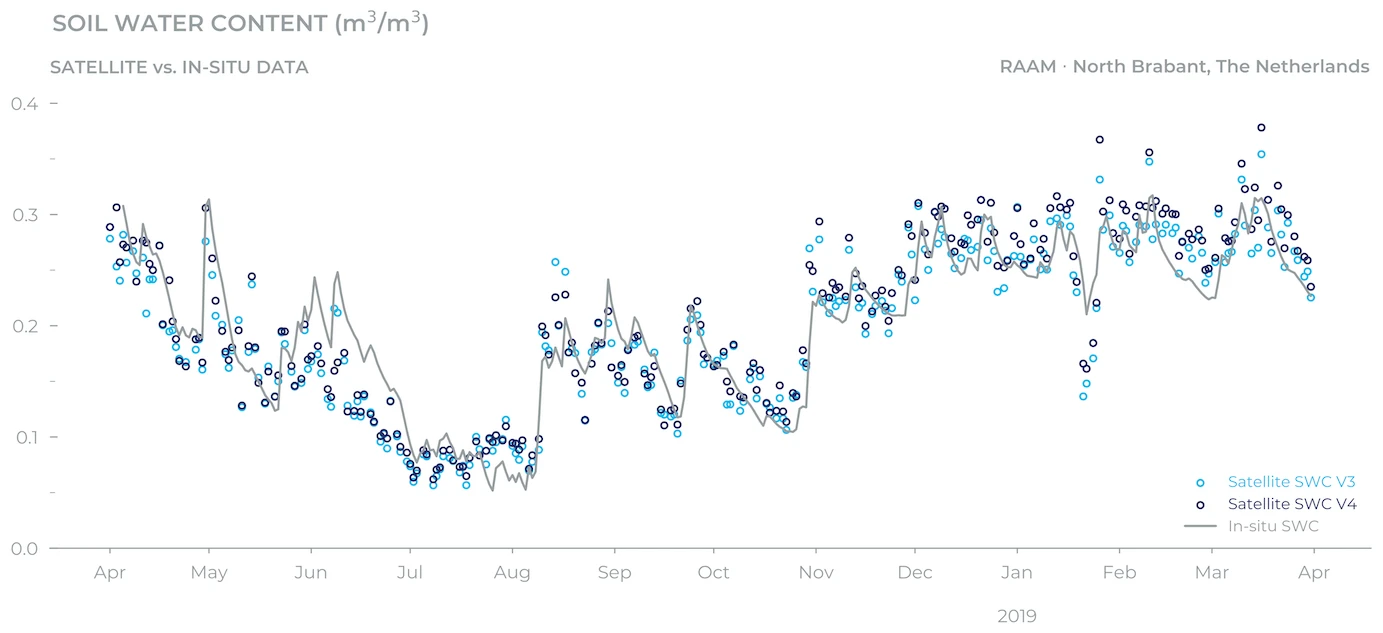
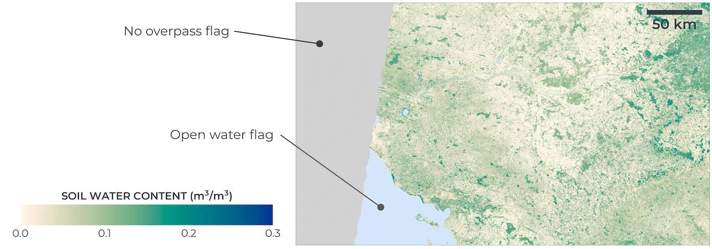
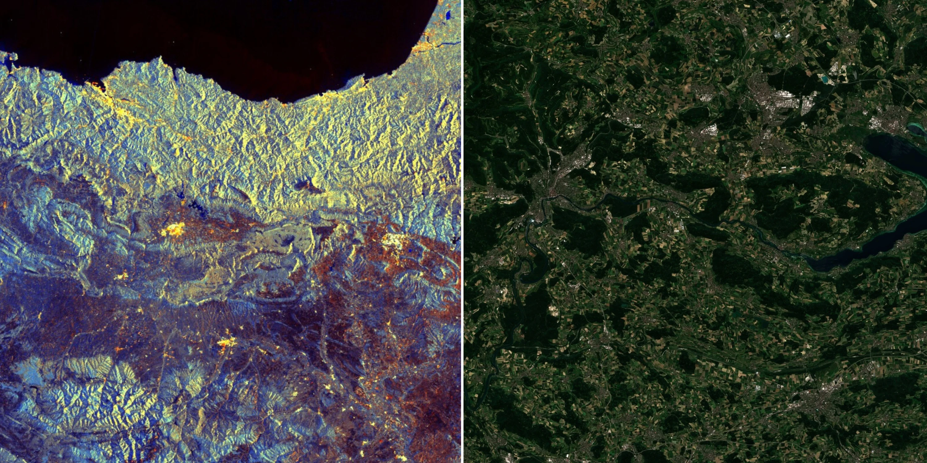
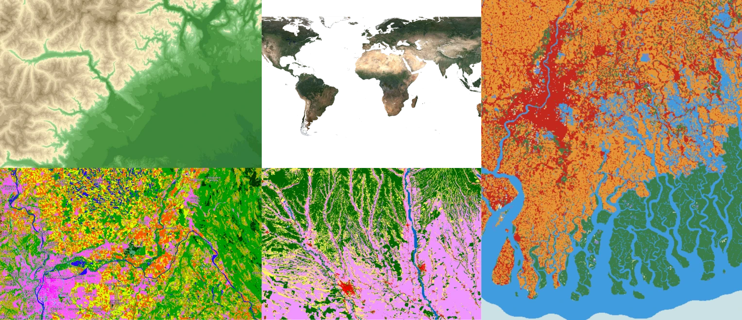
Global since January 2017 | | [Digital Elevation Model](https://docs.planet.com/data/public-data/other-datasets/dem.md) | Global digital elevation models from Copernicus and Mapzen | Global | | [BYOC](https://docs.planet.com/develop/apis/byoc.md#accessing-byoc-data) | User-provided raster data imported for processing and analysis | Depends on data | ### US-West-2 (Oregon) Regions **API endpoint:** `services-uswest2.sentinel-hub.com/` | Collection | Description | Coverage | | -------------------------------------------------------------------------------------------------------------------- | ------------------------------------------------------------------------------------------- | --------------------------------- | | [Landsat 8 L1](https://docs.planet.com/data/public-data/usgs-nasa/landsat-8-9.md) | Multispectral imagery from the Landsat 8 and 9 missions | Global since February 2013 | | [Landsat 8 L2](https://docs.planet.com/data/public-data/usgs-nasa/landsat-8-9.md) | Atmospherically corrected multispectral imagery from Landsat 8 and 9 | Global since February 2013 | | [Landsat 7 L1](https://docs.planet.com/data/public-data/usgs-nasa/landsat-7-etm.md) | Multispectral imagery from the Landsat 7 mission | Global since April 1999 | | [Landsat 7 L2](https://docs.planet.com/data/public-data/usgs-nasa/landsat-7-etm.md) | Atmospherically corrected multispectral imagery from Landsat 7 | Global since April 1999 | | [Landsat 4-5 TM L1](https://docs.planet.com/data/public-data/usgs-nasa/landsat-4-5-tm.md) | Multispectral imagery from the Landsat 4 and 5 missions (TM) | Global from July 1982 to May 2012 | | [Landsat 4-5 TM L2](https://docs.planet.com/data/public-data/usgs-nasa/landsat-4-5-tm.md) | Atmospherically corrected multispectral imagery from Landsat 4 and 5 (TM) | Global from July 1982 to May 2012 | | [Harmonized Landsat Sentinel HLS](https://docs.planet.com/data/public-data/usgs-nasa/harmonized-landsat-sentinel.md) | Harmonized surface reflectance from Landsat 8–9 OLI and Sentinel-2 MSI sensors | Global since April 2013 | | [Digital Elevation Model](https://docs.planet.com/data/public-data/other-datasets/dem.md) | Digital elevation model data by [Mapzen](https://github.com/tilezen/joerd/tree/master/docs) | Global | | [BYOC](https://docs.planet.com/develop/apis/byoc.md#accessing-byoc-data) | User-provided raster data imported for processing and analysis | Depends on data | note For consistency of the documentation all further examples will be based on `services.sentinel-hub.com/` end-point. To access Landsat or DEM data, you can simply replace “**services**” with “**services-uswest2**” to get the applicable results. --- Copy for LLM[View as Markdown](https://docs.planet.com/data/public-data/copernicus/) # Copernicus Imagery [![](/data/public-data/sentinel-1-grd/thumbnail.webp)](https://docs.planet.com/data/public-data/copernicus/sentinel-1-grd.md) ### [Sentinel 1 GRD](https://docs.planet.com/data/public-data/copernicus/sentinel-1-grd.md) [Use Processing API to access Sentinel-1 (C-band synthetic aperture radar imaging) data.](https://docs.planet.com/data/public-data/copernicus/sentinel-1-grd.md) [![](/data/public-data/sentinel-2/thumbnail.webp)](https://docs.planet.com/data/public-data/copernicus/sentinel-2.md) ### [Sentinel 2 L1C & L2A](https://docs.planet.com/data/public-data/copernicus/sentinel-2.md) [Use Processing API to access Sentinel-2 data.](https://docs.planet.com/data/public-data/copernicus/sentinel-2.md) --- Copy for LLM[View as Markdown](https://docs.planet.com/data/public-data/copernicus/sentinel-1-grd/) # Sentinel 1 GRD ![Header Thumbnail](/data/public-data/sentinel-1-grd/thumbnail.webp) Sentinel-1 imagery is provided by a constellation of polar-orbiting satellites, operating day and night performing C-band synthetic aperture radar (SAR), enabling acquisitions regardless of weather conditions. Main applications include monitoring sea ice, oil spills, marine winds, waves and currents, land-use change, land deformation, and supporting rapid response to emergencies such as floods and earthquakes. note On December 23, 2021, one of the two satellites Sentinel-1B encountered an anomaly of the power unit, causing SAR functionality to be lost, and the satellite will be intentionally deorbited in the future. Thus, between December 23, 2021 and March 26, 2025 (beginning of data availability after successful launch of Sentinel-1C [1](https://dataspace.copernicus.eu/news/2025-3-25-sentinel-1c-user-data-opening-26th-march#:~:text=Initial%20access%20to%20Sentinel%2D1C%20data%20is%20available,*%20Data%20calibration%20and%20validation%20remain%20preliminary)) only data from Sentinel-1A is available, which means some areas lost coverage completely, and many others had longer revisit times. Planet provides access to Sentinel-1 Level-1 GRD (Ground Range Detected) products only. You can explore these datasets in the [Browser](https://insights.planet.com/analyze/browser/). Sentinel-1 products are released under the [Sentinel Data Legal Notice](https://sentinels.copernicus.eu/documents/247904/690755/Sentinel_Data_Legal_Notice). ## Acquisition Modes and Polarizations Sentinel-1 operates in four acquisition modes (IW, EW, SM, WV), which determine resolution, swath width, and polarization options. ESA uses predefined [Observation Scenarios](https://sentiwiki.copernicus.eu/web/s1-mission#S1Mission-ObservationandProductionScenariosS1-Mission-Observation-and-Production-Scenarios) to schedule these acquisitions globally, ensuring systematic coverage of land, oceans, and polar regions. ![Source: European Space Agency (ESA).](/data/public-data/sentinel-1-grd/sentinel-1-mode-2025.webp) Source: European Space Agency (ESA). The figure shows the global Sentinel-1 observation scenario, with acquisition modes, polarization schemes, and orbit directions planned across different regions. This scenario ensures systematic coverage of land, ocean, and polar areas. For more information, see the [Sentinel-1 Mission Overview](https://sentiwiki.copernicus.eu/web/s1-mission) and the [Sentinel-1 Applications and User Guide](https://sentiwiki.copernicus.eu/web/s1-applications). ## Processing Sentinel-1 GRD data is processed on demand through the Processing API. By configuring processing parameters such as calibration, terrain correction, and speckle filtering, you can generate outputs ranging from minimally processed radar backscatter to fully analysis-ready products. The following steps describe the available processing operations: * **Source selection**: original or multilooked imagery is chosen depending on resolution. * **Calibration and noise removal**: radiometric calibration is applied to the selected backscatter coefficient, and thermal noise is removed. * [**Speckle filtering**](#speckle-filtering): optional speckle filtering methods are available and can be enabled through processing options. * **Radiometric terrain correction (optional)**: applies radiometric terrain correction using [area integration](https://ieeexplore.ieee.org/document/5752845) when the backscatter coefficient is set to `GAMMA0_TERRAIN`, using a [digital elevation model (DEM)](https://docs.planet.com/data/public-data/other-datasets/dem.md). * **Orthorectification (optional)**: Range-Doppler geometric terrain correction using a DEM. Processing details * Orbit files included in the products are used and sufficient for GRD applications. * Areas of border noise are masked. * Radiometric terrain correction requires orthorectification to be enabled. * DEM oversampling defaults to 2 but can be adjusted for better results at coarse resolution. ## Accessing Sentinel-1 GRD Data To access data you need to send a POST request to our `process` API. The requested data will be returned as the response to your request. Each POST request can be tailored to get you exactly the data you require. To do this requires setting various parameters which depend on the data collection you are querying. This chapter will help you understand the parameters for S1GRD data. To see examples of such requests go [here](https://docs.planet.com/data/public-data/copernicus/sentinel-1-grd/examples.md), and for an overview of all API parameters see the S1GRD [API Reference](https://docs.planet.com/develop/apis/processing/reference.md). ### Endpoint Locations | Service | Notes | | -------------------------- | ------------------------- | | services.sentinel-hub.com/ | Global since October 2014 | #### Processing Behavior * **Features:** Zooming out will use multi-looked sources at an appropriate resolution to your viewing level. You can therefore expect high quality results at all zoom levels. * **Backscatter coefficients:** We support all backscatter coefficients. ### Data type identifier: `sentinel-1-grd` Use `sentinel-1-grd` (previously `S1GRD`) as the value of the `input.data.type` parameter in your API requests. This is mandatory and will ensure you get Sentinel-1 GRD data. ### Filtering Options This chapter will explain the `input.data.dataFilter` object of the `S1GRD` `process` API. #### `mosaickingOrder` Sets the order of overlapping tiles from which the output result is mosaicked. | Value | Description | | --------------- | -------------------------------------------------------------------------- | | **mostRecent** | (default) The pixel will be selected from the most recently acquired tile. | | **leastRecent** | Similar to **mostRecent** but in reverse order. | #### `resolution` (pixel spacing) | Value | Description | | ---------- | ---------------------------------- | | **HIGH** | 10m/px for IW/SM and 25m/px for EW | | **MEDIUM** | 40m/px for IW/SM and EW | #### `acquisitionMode` Sentinel-1 operates in four different acquisition modes ([more](https://sentiwiki.copernicus.eu/web/s1-mission#S1Mission-AcquisitionModesS1-Mission-Acquisition-Modes)). | Value | Description | Polarization options | | ------ | ---------------------------------------------------------------------------------------------------------------------------------------------------------------------- | -------------------- | | **SM** | Stripmap mode ([more](https://sentiwiki.copernicus.eu/web/s1-mission#S1Mission-StripmapS1-Mission-Stripmap)). | HH+HV, VV+VH, HH, VV | | **IW** | Interferometric Wide (IW) swath mode ([more](https://sentiwiki.copernicus.eu/web/s1-mission#S1Mission-InterferometricWideSwathS1-Mission-Interferometric-Wide-Swath)). | HH+HV, VV+VH, HH, VV | | **EW** | Extra Wide (EW) swath mode ([more](https://sentiwiki.copernicus.eu/web/s1-mission#S1Mission-ExtraWideSwathS1-Mission-Extra-Wide-Swath)). | HH+HV, VV+VH, HH, VV | | **WV** | Wave mode ([more](https://sentiwiki.copernicus.eu/web/s1-mission#S1Mission-WaveS1-Mission-Wave)). | HH, VV | #### `polarization` This table contains information about the polarization two letter code used by ESA and the product's contained polarizations. | Value | Description | Notes | | ------ | --------------------- | -------------------------------------------------------- | | **SH** | HH | | | **SV** | VV | | | **DH** | HH+HV | Typical for EW acquisitions | | **DV** | VV+VH | Typical for IW acquisitions | | **HH** | Partial Dual, HH only | HH+HV was acquired, only HH is available in this product | | **HV** | Partial Dual, HV only | HH+HV was acquired, only HV is available in this product | | **VV** | Partial Dual, VV only | VV+VH was acquired, only VV is available in this product | | **VH** | Partial Dual, VH only | VV+VH was acquired, only VH is available in this product | #### `orbitDirection` | Value | Description | | -------------- | -------------------------------------------------------------------------------------- | | **ASCENDING** | Data acquired when the satellite was traveling approx. towards the Earth's North pole. | | **DESCENDING** | Data acquired when the satellite was traveling approx. towards the Earth's South pole. | #### `timeliness` | Value | | ------------ | | NRT10m | | NRT1h | | NRT3h | | Fast24h | | Offline | | Reprocessing | | ArchNormal | ### Processing Options This chapter will explain the `input.data.processing` object of the `S1GRD` `process` API. | Parameter | Description | Values | Default | | ------------------------------ | ----------------------------------------------------------------------------------------------------------------------------------------------------------------------------------------------- | ---------------------------------------------------------------------------------------------------------------------------------------------------------------------------------------------------------------------------------------------------------------------------------------------------------------- | --------------------- | | upsampling | Interpolation method used for resampling Sentinel-1 GRD data when the requested resolution differs from the source resolution. The same method is applied for both upsampling and downsampling. | **NEAREST** - [nearest neighbour interpolation](https://en.wikipedia.org/wiki/Nearest-neighbor_interpolation)

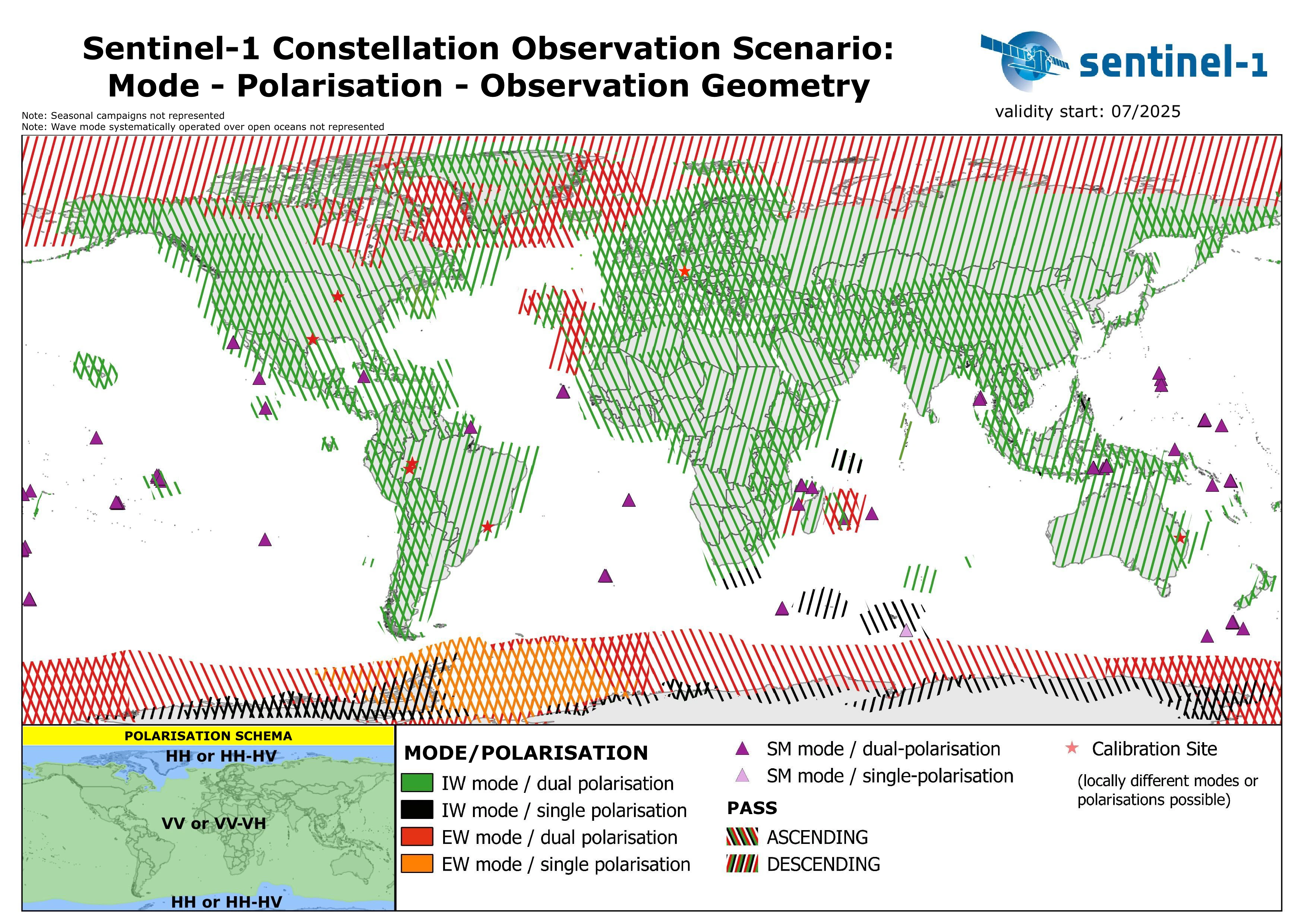
**BILINEAR** - [bilinear interpolation](https://en.wikipedia.org/wiki/Bilinear_interpolation)
**BICUBIC** - [bicubic interpolation](https://en.wikipedia.org/wiki/Bicubic_interpolation) | **NEAREST** | | backCoeff \[1] | Backscatter coefficient | **BETA0**
**SIGMA0\_ELLIPSOID**
**GAMMA0\_ELLIPSOID**
**GAMMA0\_TERRAIN** | **GAMMA0\_ELLIPSOID** | | orthorectify \[2] | Enables/disables orthorectification | **TRUE** - Orthorectified
**FALSE** - non-Orthorectified
| **FALSE** | | demInstance | The DEM used for orthorectification | **MAPZEN** - Mapzen DEM
**COPERNICUS** - Copernicus DEM 10m and 30m \[3]\[4]
**COPERNICUS\_30** - Copernicus DEM 30m \[4]
**COPERNICUS\_90** - Copernicus DEM 90m | Deployment-dependent | | radiometricTerrainOversampling | Sets the DEM oversampling parameter for radiometric terrain correction. Integer values recommended. | 1 to 4 | 2 | | speckleFilter | Defines the speckle filtering method and parameters to use. | See [Speckle Filtering](#speckle-filtering) | NONE | note * For Sentinel-1 GRD, the `downsampling` interpolation is not configurable and always uses the same method as specified for `upsampling`. * The default DEM depends on the deployment: * **EU-Central-1 (Frankfurt):** `COPERNICUS_30` * **US-West-2 (Oregon):** `MAPZEN` \[1]: `gamma0_ellipsoid` and `sigma0_ellipsoid` use an ellipsoid earth model. Radiometric terrain correction can be enabled by setting the backscatter coefficient to `gamma0_terrain`; orthorectification must be enabled in this case. \[2]: For orthorectification, we use the DEM instance specified in the demInstance field or the default DEM instance if this is not set. The Copernicus DEM is generally of higher quality and recommended in most cases. The non-orthorectified products use a simple earth model as provided in the products themselves. This may be sufficient for very flat target areas and is faster to process. \[3]: It has 10m resolution inside [39 European states including islands](https://dataspace.copernicus.eu/explore-data/data-collections/copernicus-contributing-missions/collections-description/COP-DEM) and 30m elsewhere. The 30m DEM is used exclusively if the request resolution is lower (more zoomed out) than 120m/px. \[4]: The Copernicus 30m DEM has global coverage if used for the processing of Sentinel-1 data. #### Speckle Filtering Speckle filtering is applied right after calibration and noise removal and done on source data. To enable speckle filtering, add the speckle filter object with the correct type and parameters to your processing options, as shown in [this example](https://docs.planet.com/data/public-data/copernicus/sentinel-1-grd/examples.md#s1grd-non-orthorectified-lee-speckle-filtered-decibel-gamma0-hh-between--20-db-and-10-db-png). Available filters: 1. The `NONE` filter, which as the name implies, does nothing, and is equivalent to not having the filter defined at all. ``` "speckleFilter": { "type": "NONE" } ``` 2. The LEE speckle filter. Window sizes from 1 to 7 are supported in each dimension. Odd valued window sizes are recommended. Processing time rapidly increases as window size increases. Note also that the effect of the filter depends on the resolution/zoom level; it is most pronounced at native resolution and gets reduced as you zoom out. We therefore suggest you use it at or near native resolution and switch it off at low resolution to save processing time. The effect of the filter is negligible if greatly zoomed out. An example with a 5x5 window: ``` "speckleFilter": { "type": "LEE", "windowSizeX": 5, "windowSizeY": 5 } ``` **Note:** As an alternative or in addition to this, you can also perform [multitemporal averaging](https://docs.planet.com/data/public-data/copernicus/sentinel-1-grd/examples.md#s1grd-orthorectified-gamma0-two-month-temporal-averaged-decibel-vv-between--20-db-and-0-db-png) to reduce speckle. ### Available Bands and Data Information in this chapter is useful when defining [`input` object](https://docs.planet.com/develop/evalscripts/functions.md#input-object-properties) in evalscript. Any string listed in the column **Name** can be an element of the `input.bands` array in your evalscript. | Name | Description | | ------------------- | ------------------------------------------------------------------------------------------------------------------------------------------------------------------------------------------------------------------------------------------------------- | | VV | Present when the product polarization type is one of SV, DV or VV. | | VH | Present when the product polarization type is VH or DV. | | HV | Present when the product polarization type is HV or DH. | | HH | Present when the product polarization type is one of SH, DH or HH. | | localIncidenceAngle | The local incidence angle for each output pixel. Only available if orthorectification is enabled. | | scatteringArea | The normalized scattering area for each output pixel. Used for conversion of beta0 to terrain corrected gamma0. Only available if radiometric terrain correction is performed. | | shadowMask | Flags output pixels which are in or near radar shadow. Is `true` if the nearest GRD source pixel is at most one GRD pixel away from a GRD pixel with a scatteringArea of less than 0.05. Only available if radiometric terrain correction is performed. | | dataMask | The mask of data/nodata pixels ([more](https://docs.planet.com/develop/evalscripts.md#data-mask)). | ### Units The data values for each band in your custom script are presented in the units as specified here. In case more than one unit is available for a given band, you may optionally set the value of `input.units` in your evalscript `setup` function to one of the values in the `Units Value` column. Doing so will present data in that unit. The `units` parameter combines the physical quantity and corresponding units of measurement values. As such, some names more closely resemble physical quantities, others resemble units of measurement. The `Source Format` specifies how and with what precision the digital numbers (`DN`) from which the unit is derived are encoded. Bands requested in `DN` units contain exactly the pixel values of the source data. Note that resampling may produce interpolated values. `DN` is also used whenever a band is derived computationally (like dataMask); such bands can be identified by having `DN` units and `N/A` source format. `DN` values are typically not offered if they do not simply represent any physical quantity, in particular, when `DN` values require source-specific (i.e. non-global) conversion to physical quantities. Values in non-`DN` units are computed from the source (`DN`) values with at least float32 precision. Note that the conversion might be nonlinear, therefore the full value range and quantization step size of such a band can be hard to predict. Band values in evalscripts always behave as floating point numbers, regardless of the actual precision. The `Typical Range` indicates what values are common for a given band and unit, however outliers can be expected. For Sentinel-1, data values are linear power in the chosen backscatter coefficient. To specify the backscatter coefficient, set `BETA0`, `SIGMA0_ELLIPSOID`, `GAMMA0_ELLIPSOID` (default) or `GAMMA0_TERRAIN` as the value of `input.data.processing.backCoeff` in your request. The default is `GAMMA0_ELLIPSOID`. | Band | Physical Quantity (units) | Units Value | Source Format | Typical Range | Notes | | -------------------------------- | ------------------------------------------------------------- | ------------- | ------------- | ---------------------------------------------------------------- | -------------------------------------------------------------------------------------------------------------------------------------------------- | | Polarization
VV, HH, VH, HV | Linear power in the chosen backscatter coefficient (unitless) | LINEAR\_POWER | UINT16 | 0 - 0.5 | Can reach very high values (such as 1000); for visualizing a large dynamic range consider converting to decibels: `decibel = 10 * log10 (linear)`. | | localIncidenceAngle | Angle (degrees) | DN | N/A | 0 - 180 | Computed for each output pixel. Requires orthorectification. | | scatteringArea | Normalized area (unitless) | DN | N/A | 0 - 2 | Can reach high values on foreslopes. Requires radiometric terrain correction. | | shadowMask | N/A | DN | N/A | 0 - likely not radar shadow
1 - likely in/near radar shadow | Requires radiometric terrain correction. | | dataMask | N/A | DN | N/A | 0 - no data
1 - data | | ### Scenes Object [`scenes` object](https://docs.planet.com/develop/evalscripts/functions.md#scenes) stores metadata. An example of metadata available in `scenes` object for Sentinel-1 GRD when mosaicking is `ORBIT`: | Property name | Value | | ---------------------------- | --------------------------------------------------------------------------------------------------------------- | | dateFrom | `'2019-04-02T00:00:00Z'` | | dateTo | `'2019-04-02T23:59:59Z'` | | tiles\[i].sentinel1ProductId | `'S1A_IW_GRDH_1SDV_20190402T170539_20190402T170604_026614_02FC31_7D8E'` | | tiles\[i].date | `'2019-04-02T17:05:39Z'` | | tiles\[i].shId | `881338` | | tiles\[i].dataPath | `'s3://sentinel-s1-l1c/GRD/2019/4/2/IW/DV/S1A_IW_GRDH_1SDV_20190402T170539_20190402T170604_026614_02FC31_7D8E'` | Properties of a `scenes` object can differ depending on the selected mosaicking and in which evalscript function the object is accessed. [Working with metadata in evalscript](https://docs.planet.com/develop/evalscripts.md#working-with-metadata-in-evalscripts) user guide explains all details and provide examples. ### Mosaicking `SIMPLE` and `ORBIT` [mosaicking](https://docs.planet.com/develop/evalscripts/functions.md#mosaicking) types are supported. `TILE` mosaicking is not supported for this collection. ## Collection specific constraints * **Noise**: Thermal noise reduction is applied to all Sentinel-1 GRD products. * **Decibel units**: For decibel outputs, a conversion is necessary within your evalscript, see an example [here](https://docs.planet.com/data/public-data/copernicus/sentinel-1-grd/examples.md#s1grd-orthorectified-decibel-gamma0-vh-between--20-db-and-0-db-png). We offer pre-defined evalscripts, which return S1GRD values in decibel units, as products in the Configuration Utility for your convenience. * **Orbit state vectors**: We currently use the orbit state vectors provided in the products themselves as we find these sufficient for GRD use. ## CARD4L Data CARD4L or [CEOS Analysis Ready Data](https://ceos.org/ard/) for Land refers to Sentinel-1 satellite data that has been processed to a predefined set of requirements (specifically [Normalised Radar Backscatter](https://ceos.org/ard/files/PFS/NRB/v5.5/CARD4L-PFS_NRB_v5.5.pdf) requirements), making Sentinel-1 data analysis ready and thus reducing its complexity. It is especially useful for non-expert users, as it does most of the data preparation work in advance, including geometric and radiometric correction. CARD4L also takes care of obligatory and extensive metadata generation, detailing data provenance, processing parameters, etc. We have created a [CARD4L request generation tool](https://apps.sentinel-hub.com/s1-card4l/), which makes it easy to process CARD4L [compliant](https://ceos.org/ard/files/Self%20Assessments/NRB/v5.5/WGCV_CARD4L_Assessment_for_Sinergise_Sentinel-1_NRB_v5.5.pdf) Sentinel-1 data. To use it, you will need an [enterprise account](https://www.planet.com/pricing/?tab=platform), which activates access to batch processing. Note that you can get the equivalent raster data with the correct settings in an API request yourself, however metadata can only be obtained using the tool. **Articles and use cases** * We are processing Sentinel-1 CARD4L data for the [Digital Earth Africa project](https://docs.digitalearthafrica.org/en/latest/index.html). Technical information about the data and how to access it may be found [here](https://docs.digitalearthafrica.org/en/latest/data_specs/Sentinel-1_specs.html). * [An Operational Analysis Ready Radar Backscatter Dataset for the African Continent](https://www.mdpi.com/2072-4292/14/2/351), January 2022 * [Intercomparison of Sentinel-1 Datasets from Google Earth Engine and the Card4L Tool](https://www.researchgate.net/publication/355208945_Intercomparison_of_Sentinel-1_Datasets_from_Google_Earth_Engine_and_the_Sinergise_Sentinel_Hub_Card4L_Tool), July 2021 ## Catalog API Capabilities To access Sentinel-1 GRD product metadata you need to send search request to our [Catalog API](https://docs.planet.com/develop/apis/catalog/reference.md). The requested metadata will be returned as JSON formatted response to your request. This chapter will help with understanding Sentinel 1 GRD specific parameters for search request. ### Collection identifier: `sentinel-1-grd` ### Filter extension * `sar:instrument_mode` ([possible values](#acquisitionmode)) * `sat:orbit_state` ([possible values](#orbitdirection)) * `s1:polarization` ([possible values](#polarization)) * `s1:resolution` ([possible values](#resolution-pixel-spacing)) * `s1:timeliness` ([possible values](#timeliness)) ### Distinct extension * `date` * `sar:instrument_mode` * `sat:orbit_state` * `s1:polarization` --- Copy for LLM[View as Markdown](https://docs.planet.com/data/public-data/copernicus/sentinel-1-grd/examples/) # Sentinel 1 GRD Examples The following examples are CURL requests and can be run from the command line or terminal. In addition, you can copy and paste these examples into [Request Builder](https://insights.planet.com/analyze/requests-builder/). You can translate the requests into other programming languages in the Request Builder app. To request data using any of the request below, you will need to replace the string `` with your access token. Your access token will look something like this: ``` ayJhbGciOiJSUzI1NiJ9.ayJzdWIiOiI0MmYwODZjCy1kMzI3LTRlOTMtYWMxNS00ODAwOGFiZjI0YjIiLCJhdWQiOiJlY2I1MGM1Zi1i MWM1LTQ3ZTgtYWE4NC0zZTU4NzJlM2I2MTEiLCJqdGkiOiI5MzYxMWE4ODEyNTM4Y2M0MmU0NDJjYjUyMTY0YmJlNyIsImV4cCI6MTU1N TQyMzk3MiwibmFtZSI6ImFuamEudnJlY2tvQHNpbmVyZ2lzZS5jb20iLCJlbWFpbCI6ImFuamEudnJlY2tvQHNpbmVyZ2lzZS5jb20iLC JzaWQiOiIzZjVjZDVkNS04MjRiLTQ3ZjYtODgwNy0wNDMyNWY4ODQxZmQifQ.U7FPOy_2jlEOFxXSjyN5KEdBROna3-Dyec0feShIbUOY 1p9lEXdNaMmR5euiINi2RXDayX9Kr47CuSTsvq1zHFvZs1YgkFr1iH6kDuX-t_-wfWpqu5oPjoPVKZ4Rj0Ms_dxAUTQFTXR0rlbLuO-KS gnaeLVb5iiv_qY3Ctq2XKdIRcFRQLFziFcP4yZJl-NZMlwzsiiwjakcpYpI5jSYAdU2hpZLHRzceseeZt5YfZOe5Px1kZXro9Nd0L2GPC -qzOXw_V1saMGFa2ov8qV6Dvk92iv2SDDdGhOdII_JOf8XkK4E3g2z0EEFdWhG9F4Iky4ukNsqBPgE8LRb31s0hg ``` and can be obtained as described in the [Authentication chapter](https://docs.planet.com/develop/authentication.md). ## S1GRD orthorectified linear gamma0 VV between 0 and 0.5 (png) ``` curl -X POST \ https://services.sentinel-hub.com/process/v1 \ -H 'Authorization: Bearer ' \ -F 'request={ "input": { "bounds": { "bbox": [ 1360000,5121900,1370000,5131900 ], "properties": { "crs": "http://www.opengis.net/def/crs/EPSG/0/3857" } }, "data": [ { "type": "sentinel-1-grd", "dataFilter": { "timeRange": { "from": "2019-02-02T00:00:00Z", "to": "2019-04-02T23:59:59Z" } }, "processing": { "orthorectify": "true" } } ] }, "output": { "width": 512, "height": 512, "responses": [ { "identifier": "default", "format": { "type": "image/png" } } ] } }' \ -F 'evalscript=//VERSION=3 function setup() { return { input: ["VV"], output: { id:"default", bands: 1} } } function evaluatePixel(samples) { return [2 * samples.VV] }' ``` ## S1GRD orthorectified linear gamma0 VV between 0 and 0.5 in approximate real-world 10 m resolution (IW) (png) ``` curl -X POST \ https://services.sentinel-hub.com/process/v1 \ -H 'Authorization: Bearer ' \ -F 'request={ "input": { "bounds": { "bbox": [ 268574.43, 4624494.84, 276045.41, 4631696.16 ], "properties": { "crs": "http://www.opengis.net/def/crs/EPSG/0/32633" } }, "data": [{ "dataFilter": { "timeRange": { "from": "2019-02-02T00:00:00Z", "to": "2019-04-02T23:59:59Z" }, "resolution": "HIGH", "acquisitionMode": "IW" }, "processing": { "orthorectify": "true", "demInstance": "COPERNICUS_30" }, "type": "sentinel-1-grd" }] }, "output": { "resx": 10, "resy": 10, "responses": [{ "identifier": "default", "format": { "type": "image/png" } }] } }' \ -F 'evalscript=//VERSION=3 function setup() { return { input: ["VV"], output: { id:"default", bands: 1} } } function evaluatePixel(samples) { return [2 * samples.VV] }' ``` ## S1GRD orthorectified with Copernicus DEM 30 (png) ``` curl -X POST \ https://services.sentinel-hub.com/process/v1 \ -H 'Authorization: Bearer ' \ -F 'request={ "input": { "bounds": { "bbox": [ 1360000,5121900,1370000,5131900 ], "properties": { "crs": "http://www.opengis.net/def/crs/EPSG/0/3857" } }, "data": [ { "type": "sentinel-1-grd", "dataFilter": { "timeRange": { "from": "2019-02-02T00:00:00Z", "to": "2019-04-02T23:59:59Z" } }, "processing": { "orthorectify": "true", "demInstance": "COPERNICUS_30" } } ] }, "output": { "width": 512, "height": 512, "responses": [ { "identifier": "default", "format": { "type": "image/png" } } ] } }' \ -F 'evalscript=//VERSION=3 function setup() { return { input: ["VV"], output: { id:"default", bands: 1} } } function evaluatePixel(samples) { return [2 * samples.VV] }' ``` ## S1GRD orthorectified linear gamma0 VV, ascending orbit direction, GeoTIFF in EPSG:32648 (UTM zone 48N) ``` curl -X POST \ https://services.sentinel-hub.com/process/v1 \ -H 'Accept: image/tiff' \ -H 'Authorization: Bearer ' \ -F 'request={ "input": { "bounds": { "bbox": [ 699800, 1190220, 709800, 1200220 ], "properties": { "crs": "http://www.opengis.net/def/crs/EPSG/0/32648" } }, "data": [ { "type": "sentinel-1-grd", "dataFilter": { "timeRange": { "from": "2017-11-15T00:00:00Z", "to": "2017-11-15T23:00:00Z" }, "acquisitionMode": "IW", "polarization": "DV", "orbitDirection ": "ASCENDING" }, "processing": { "backCoeff": "GAMMA0_ELLIPSOID", "orthorectify": "true" } } ] }, "output": { "width": 1000, "height": 1000, "responses": [ { "identifier": "default", "format": { "type": "image/tiff" } } ] } }' \ -F 'evalscript=//VERSION=3 function setup() { return { input: ["VV"], output: { id:"default", bands: 1,sampleType: SampleType.FLOAT32} } } function evaluatePixel(samples) { return [samples.VV] }' ``` ## S1GRD orthorectified decibel gamma0 VH between -20 dB and 0 dB (png) ``` curl -X POST \ https://services.sentinel-hub.com/process/v1 \ -H 'Authorization: Bearer ' \ -F 'request={ "input": { "bounds": { "bbox": [ 1360000,5121900,1370000,5131900 ], "properties": { "crs": "http://www.opengis.net/def/crs/EPSG/0/3857" } }, "data": [ { "type": "sentinel-1-grd", "dataFilter": { "timeRange": { "from": "2019-02-02T00:00:00Z", "to": "2019-04-02T23:59:59Z" } }, "processing": { "orthorectify": "true" } } ] }, "output": { "width": 512, "height": 512, "responses": [ { "identifier": "default", "format": { "type": "image/png" } } ] } }' \ -F 'evalscript=//VERSION=3 function setup() { return { input: ["VH"], output: { id:"default", bands: 1} } } function evaluatePixel(samples) { return [toDb(samples.VH)] } // visualizes decibels from -20 to 0 function toDb(linear) { // the following commented out lines are simplified below // var log = 10 * Math.log(linear) / Math.LN10 // var val = Math.max(0, (log + 20) / 20) return Math.max(0, Math.log(linear) * 0.21714724095 + 1) }' ``` ## S1GRD orthorectified decibel gamma0 RGB composite of VV, VH, VV/VH/10 between -20 dB and 0 dB (png) ``` curl -X POST \ https://services.sentinel-hub.com/process/v1 \ -H 'Authorization: Bearer ' \ -F 'request={ "input": { "bounds": { "bbox": [ 1360000,5121900,1370000,5131900 ], "properties": { "crs": "http://www.opengis.net/def/crs/EPSG/0/3857" } }, "data": [ { "type": "sentinel-1-grd", "dataFilter": { "timeRange": { "from": "2019-02-02T00:00:00Z", "to": "2019-04-02T23:59:59Z" } }, "processing": { "orthorectify": "true" } } ] }, "output": { "width": 512, "height": 512, "responses": [ { "identifier": "default", "format": { "type": "image/png" } } ] } }' \ -F 'evalscript=//VERSION=3 function setup() { return { input: ["VV", "VH"], output: { id:"default", bands: 3} } } function evaluatePixel(samples) { var vvdB = toDb(samples.VV) var vhdB = toDb(samples.VH) return [vvdB, vhdB, vvdB / vhdB / 10] } // displays VV in decibels from -20 to 0 function toDb(linear) { // the following commented out lines are simplified below // var log = 10 * Math.log(linear) / Math.LN10 // var val = Math.max(0, (log + 20) / 20) return Math.max(0, Math.log(linear) * 0.21714724095 + 1) }' ``` ## S1GRD non-orthorectified linear sigma0 VH between 0 and 0.5 (png) ``` curl -X POST \ https://services.sentinel-hub.com/process/v1 \ -H 'Authorization: Bearer ' \ -F 'request={ "input": { "bounds": { "bbox": [ 1360000,5121900,1370000,5131900 ], "properties": { "crs": "http://www.opengis.net/def/crs/EPSG/0/3857" } }, "data": [ { "type": "sentinel-1-grd", "dataFilter": { "timeRange": { "from": "2019-02-02T00:00:00Z", "to": "2019-04-02T23:59:59Z" } }, "processing": { "orthorectify": "false", "backCoeff": "SIGMA0_ELLIPSOID" } } ] }, "output": { "width": 512, "height": 512, "responses": [ { "identifier": "default", "format": { "type": "image/png" } } ] } }' \ -F 'evalscript=//VERSION=3 function setup() { return { input: ["VH"], output: { id:"default", bands: 1} } } function evaluatePixel(samples) { return [2 * samples.VH] }' ``` ## S1GRD non-orthorectified Lee speckle filtered decibel gamma0 HH between -20 dB and +10 dB (png) ``` curl -X POST \ https://services.sentinel-hub.com/process/v1 \ -H 'Authorization: Bearer ' \ -F 'request={ "input": { "bounds": { "bbox": [ 18400000,-11330000,18500000,-11430000 ], "properties": { "crs": "http://www.opengis.net/def/crs/EPSG/0/3857" } }, "data": [ { "type": "sentinel-1-grd", "dataFilter": { "acquisitionMode": "EW", "timeRange": { "from": "2020-09-29T00:00:00Z", "to": "2020-09-29T23:59:59Z" } }, "processing": { "orthorectify": "false", "backCoeff": "GAMMA0_ELLIPSOID", "speckleFilter": { "type": "LEE", "windowSizeX": 5, "windowSizeY": 5 } } } ] }, "output": { "width": 1000, "height": 1000, "responses": [ { "identifier": "default", "format": { "type": "image/png" } } ] } }' \ -F 'evalscript=//VERSION=3 function setup() { return { input: ["HH"], output: { id:"default", bands: 1} } } function evaluatePixel(samples) { return [toDb(samples.HH)] } // visualizes decibels from -20 to +10 function toDb(linear) { var log = 10 * Math.log(linear) / Math.LN10 return Math.max(0, (log + 20) / 30) }' ``` ## S1GRD orthorectified gamma0 two month temporal averaged decibel VV between -20 dB and 0 dB (png) ``` curl -X POST \ https://services.sentinel-hub.com/process/v1 \ -H 'Authorization: Bearer ' \ -F 'request={ "input": { "bounds": { "bbox": [ 1360000,5121900,1370000,5131900 ], "properties": { "crs": "http://www.opengis.net/def/crs/EPSG/0/3857" } }, "data": [ { "type": "sentinel-1-grd", "dataFilter": { "timeRange": { "from": "2019-02-01T00:00:00Z", "to": "2019-04-02T23:59:59Z" }, "orbitDirection": "ASCENDING" }, "processing": { "orthorectify": "true" } } ] }, "output": { "width": 512, "height": 512, "responses": [ { "identifier": "default", "format": { "type": "image/png" } } ] } }' \ -F 'evalscript=//VERSION=3 function setup() { return { input: ["VV", "dataMask"], output: { id:"default", bands: 1}, mosaicking: Mosaicking.ORBIT } } function evaluatePixel(samples) { return [calculateAverage(samples)] } function calculateAverage(samples) { var sum = 0 var nValid = 0 for (let sample of samples) { if (sample.dataMask != 0) { nValid++ sum += toDb(sample.VV) } } return sum / nValid } // visualizes decibels from -20 to 0 function toDb(linear) { // the following commented out lines are simplified below // var log = 10 * Math.log(linear) / Math.LN10 // var val = Math.max(0, (log + 20) / 20) return Math.max(0, Math.log(linear) * 0.21714724095 + 1) }' ``` ## S1GRD radiometrically terrain corrected linear gamma0 VV between 0 and 0.5 (png) ``` curl -X POST \ https://services.sentinel-hub.com/process/v1 \ -H 'Authorization: Bearer ' \ -F 'request={ "input": { "bounds": { "bbox": [ 1095431, 5714610, 1146158, 5754129 ], "properties": { "crs": "http://www.opengis.net/def/crs/EPSG/0/3857" } }, "data": [ { "type": "sentinel-1-grd", "dataFilter": { "timeRange": { "from": "2019-02-02T00:00:00Z", "to": "2019-04-02T23:59:59Z" } }, "processing": { "orthorectify": "true", "backCoeff": "GAMMA0_TERRAIN" } } ] }, "output": { "width": 512, "height": 512, "responses": [ { "identifier": "default", "format": { "type": "image/png" } } ] } }' \ -F 'evalscript=//VERSION=3 function setup() { return { input: ["VV"], output: { id:"default", bands: 1} } } function evaluatePixel(samples) { return [2 * samples.VV] }' ``` ## S1GRD radiometrically terrain corrected using Copernicus DEM 30 (png) ``` curl -X POST \ https://services.sentinel-hub.com/process/v1 \ -H 'Authorization: Bearer ' \ -F 'request={ "input": { "bounds": { "bbox": [ 1095431, 5714610, 1146158, 5754129 ], "properties": { "crs": "http://www.opengis.net/def/crs/EPSG/0/3857" } }, "data": [ { "type": "sentinel-1-grd", "dataFilter": { "timeRange": { "from": "2019-02-02T00:00:00Z", "to": "2019-04-02T23:59:59Z" } }, "processing": { "orthorectify": "true", "backCoeff": "GAMMA0_TERRAIN", "demInstance": "COPERNICUS_30" } } ] }, "output": { "width": 512, "height": 512, "responses": [ { "identifier": "default", "format": { "type": "image/png" } } ] } }' \ -F 'evalscript=//VERSION=3 function setup() { return { input: ["VV"], output: { id:"default", bands: 1} } } function evaluatePixel(samples) { return [2 * samples.VV] }' ``` ## S1GRD radiometrically terrain corrected with custom DEM oversampling of 3 (png) ``` curl -X POST \ https://services.sentinel-hub.com/process/v1 \ -H 'Authorization: Bearer ' \ -F 'request={ "input": { "bounds": { "bbox": [ 1095431, 5714610, 1146158, 5754129 ], "properties": { "crs": "http://www.opengis.net/def/crs/EPSG/0/3857" } }, "data": [ { "type": "sentinel-1-grd", "dataFilter": { "timeRange": { "from": "2019-02-02T00:00:00Z", "to": "2019-04-02T23:59:59Z" } }, "processing": { "orthorectify": "true", "backCoeff": "GAMMA0_TERRAIN", "radiometricTerrainOversampling": 3 } } ] }, "output": { "width": 512, "height": 512, "responses": [ { "identifier": "default", "format": { "type": "image/png" } } ] } }' \ -F 'evalscript=//VERSION=3 function setup() { return { input: ["VV"], output: { id:"default", bands: 1} } } function evaluatePixel(samples) { return [2 * samples.VV] }' ``` ## S1GRD radiometrically terrain corrected gamma0 VV and auxiliary data: local incidence angle, scattering area, and shadow mask ``` curl -X POST \ https://services.sentinel-hub.com/process/v1 \ -H 'Authorization: Bearer ' \ -H 'Accept: application/tar' \ -F 'request={ "input": { "bounds": { "bbox": [ 565556.94, 5048644.47, 600656.56, 5076658.33 ], "properties": { "crs": "http://www.opengis.net/def/crs/EPSG/0/32632" } }, "data": [ { "type": "sentinel-1-grd", "dataFilter": { "timeRange": { "from": "2019-02-02T00:00:00Z", "to": "2019-04-02T23:59:59Z" } }, "processing": { "orthorectify": "true", "backCoeff": "GAMMA0_TERRAIN" } } ] }, "output": { "width": 1024, "height": 796, "responses": [ { "identifier": "s1_rtc_VV_area", "format": { "type": "image/tiff" } }, { "identifier": "s1_rtc_angle_mask", "format": { "type": "image/tiff" } } ] } }' \ -F 'evalscript=//VERSION=3 function setup() { return { input: ["VV", "localIncidenceAngle", "scatteringArea", "shadowMask"], output: [{ id:"s1_rtc_VV_area", bands: 2, sampleType: "FLOAT32"}, { id:"s1_rtc_angle_mask", bands: 2, sampleType: "UINT8"}] } } function evaluatePixel(samples) { return { s1_rtc_VV_area: [samples.VV, samples.scatteringArea], s1_rtc_angle_mask: [samples.localIncidenceAngle, samples.shadowMask] } }' ``` --- Copy for LLM[View as Markdown](https://docs.planet.com/data/public-data/copernicus/sentinel-2/) # Sentinel 2 L1C & L2A ![Header Thumbnail](/data/public-data/sentinel-2/thumbnail.webp) Sentinel-2 is a European wide-swath, high-resolution (as defined by ESA) multispectral imaging mission. Its optical imagery supports applications such as land monitoring, emergency response, and security-related use cases. The multispectral instrument provides 13 spectral bands spanning the visible, near-infrared, and shortwave infrared regions. Dedicated to supplying data for Copernicus services, Sentinel-2 carries a range of technologies such as multispectral imaging instruments for land, ocean, and atmospheric monitoring. It delivers high-resolution optical images for land monitoring, emergency response, and security services. For more information, see the [S2 Mission](https://sentiwiki.copernicus.eu/web/s2-mission) and the [Collection User Guide](https://sentiwiki.copernicus.eu/web/s2-applications). ## Basic Facts | Property | Value | | ---------------------- | --------------------------------------------------------------------------------------------------------------------------------------------------------------------------- | | **Sensor** | MultiSpectral Instrument (MSI), 13 bands: four visible bands, six near-infrared bands, and three short-wave infrared bands | | **Spatial resolution** | 10 m, 20 m, and 60 m (band-dependent) | | **Revisit time** | five days at the equator (two to three days at mid latitudes) | | **Spatial coverage** | [Land and coastal areas between latitudes 56°S and 83°N](https://sentiwiki.copernicus.eu/web/s2-mission#S2Mission-GeographicalCoverageS2-Mission-Geographical-Coveragetrue) | | **Common use cases** | Land-cover mapping, land-change detection, vegetation monitoring, burned-area analysis | ### Product Differences | Property | Sentinel-2 L1C | Sentinel-2 L2A | | --------------------- | ----------------------------------- | ------------------------------------------------------------------------ | | **Measurement** | Top-of-atmosphere (TOA) reflectance | Bottom-of-atmosphere (BOA) reflectance, processed from L1C using Sen2Cor | | **Data availability** | Available since November 2015 | Available since October 2016 (global availability since January 2017) | **Note:** Sentinel-2A was maneuvered into a new orbit (located 36° away from Sentinel-2B) and resumed observations in 13 March 2025. With this campaign, the Sentinel-2 constellation consists of 3 satellites for 1 year (till 13 March 2026).[\[1\]](https://sentinels.copernicus.eu/web/sentinel/-/sentinel-2a-extended-campaign-starting-march-13-2025) ## Attribution and Use EU law grants free access to Copernicus Sentinel Data and Service Information for the purpose of the following lawful uses: a) reproduction; b) distribution; c) communication to the public; d) adaptation, modification, and combination with other data and information; e) any combination of points a to d. See more details on the [use of Copernicus Sentinel data and service information.](https://sentinels.copernicus.eu/documents/247904/690755/Sentinel_Data_Legal_Notice) Tracing based on Sentinel imagery is allowed for commercial purposes as well. **Acknowledgment**: Contains modified Copernicus Sentinel data \[Year] processed by Planet. ## Accessing Sentinel-2 Data To access data, you need to send a POST request to the Processing API. The requested data will be returned as the response to your request. Each POST request can be tailored to get exactly the data you require by setting various parameters depending on the data source. ### Endpoint Locations | Data | Service | Notes | | -------------- | -------------------------- | --------------------------------------------------------- | | Sentinel-2 L1C | services.sentinel-hub.com/ | Global since November 2015 | | Sentinel-2 L2A | services.sentinel-hub.com/ | Europe since November 2016

Global since January 2017 | **Data type identifiers:** * `sentinel-2-l1c` * `sentinel-2-l2a` Use these as the value of the `input.data.type` parameter in your API requests. This ensures you get the correct Sentinel-2 data level. ### Filtering Options This chapter explains the `input.data.dataFilter` object for Sentinel-2 data. #### `mosaickingOrder` Sets the order of overlapping tiles from which the output result is mosaicked. Tiles typically come from the same orbit/acquisition. | Value | Description | Notes | | --------------- | ------------------------------------------------------------- | --------------------------------------------------------------------------------------------------- | | **mostRecent** | (default) Pixel selected from the most recently acquired tile | In case multiple tiles share the same timestamp, the one downloaded or created latest will be used. | | **leastRecent** | Same as above, but in reverse order | | | **leastCC** | Pixel selected from tile with least cloud coverage | Tile-level metadata (each covering about 12,000 sq. km), approximate values | #### `maxCloudCoverage` Sets the upper limit for cloud coverage (%) based on precomputed estimates in the tile metadata. For example, setting `20` retrieves only tiles with at most 20% cloud coverage. note The filter is per-tile and might not perfectly reflect the area of interest. ### Rendering Limits #### Sentinel-2 L1C Rendering is available up to 200 m/px. #### Sentinel-2 L2A Rendering is available up to 1500 m/px. ### Antimeridian handling [Browser](https://insights.planet.com/analyze/browser/) does not magically handle all aspects of data which crosses the antimeridian. Longitudes beyond +180 degrees are NOT treated as longitudes beyond -180 degrees. Sentinel-2 tiles do cross the antimeridian and L1C and L2A tiles are distributed in the UTM projection. Requesting data in the native UTM coordinates will work exactly as expected. However, for mosaicking, UTM zone 1 and UTM zone 60 are not seen as intersecting even though they do intersect in reality. UTM tiles reprojected to some other coordinate system may fall outside the bounds of this coordinate system. This happens with WGS84, for example, where you may get data at -181 longitude. It is also possible to not get data at +179 longitude due to the slight asymmetry of the Sentinel-2 tile grid. In these situations some additional care must be taken when creating requests. ### Processing Options This chapter explains the `input.data.processing` object for Sentinel-2 data. | Parameter | Description | Values | Default | | ------------ | ------------------------------------------------------------- | ---------------------------------------------------------------------------------------------------------------------------------------------------------------------------------------------------------------------------------------------------------------------------------------------------------------- | ----------- | | upsampling | Interpolation when requested resolution `>` source resolution | **NEAREST** - [nearest neighbour interpolation](https://en.wikipedia.org/wiki/Nearest-neighbor_interpolation)
**BILINEAR** - [bilinear interpolation](https://en.wikipedia.org/wiki/Bilinear_interpolation)
**BICUBIC** - [bicubic interpolation](https://en.wikipedia.org/wiki/Bicubic_interpolation) | **NEAREST** | | downsampling | Interpolation when requested resolution `<` source resolution | **NEAREST** - [nearest neighbour interpolation](https://en.wikipedia.org/wiki/Nearest-neighbor_interpolation)
**BILINEAR** - [bilinear interpolation](https://en.wikipedia.org/wiki/Bilinear_interpolation)
**BICUBIC** - [bicubic interpolation](https://en.wikipedia.org/wiki/Bicubic_interpolation) | **NEAREST** | For visualization, see [upsampling comparison examples.](https://en.wikipedia.org/wiki/Comparison_gallery_of_image_scaling_algorithms) ### Available Bands and Data This chapter will explain the bands and data which can be set in the [evalscript input object](https://docs.planet.com/develop/evalscripts/functions.md#input-object-properties). Any string listed in the column **Name** can be an element of the `input.bands` array in your evalscript. | Name | Description | Resolution | Notes | | ---------------- | ---------------------------------------------------------------------------------------------- | ---------- | --------------------------------------------------------------------------------- | | B01 | Coastal aerosol | 60 m | | | B02 | Blue | 10 m | | | B03 | Green | 10 m | | | B04 | Red | 10 m | | | B05 | Vegetation red edge | 20 m | | | B06 | Vegetation red edge | 20 m | | | B07 | Vegetation red edge | 20 m | | | B08 | NIR | 10 m | | | B8A | Narrow NIR | 20 m | | | B09 | Water vapour | 60 m | | | B10 | SWIR – Cirrus | 60 m | (excluded for L2A BOA data) | | B11 | SWIR | 20 m | | | B12 | SWIR | 20 m | | | CLP | Cloud probability (S2Cloudless) ([more](#cloud-masks)) | 160 m | S2Cloudless band is 160 m; can be requested for products at any output resolution | | CLM | Cloud mask (S2Cloudless) ([more](#cloud-masks)) | 160 m | | | AOT (L2A) | Aerosol Optical Thickness map (Sen2Cor) | 10 m | Only L2A | | SCL (L2A) | Scene classification (Sen2Cor) | 20 m | Only L2A | | SNW (L2A) | Snow probability (Sen2Cor) | 20 m | Only L2A | | CLD (L2A) | Cloud probability (Sen2Cor) | 20 m | Only L2A | | sunAzimuthAngles | Sun azimuth angle | 5000 m | | | sunZenithAngles | Sun zenith angle | 5000 m | | | viewAzimuthMean | Viewing azimuth angle | 5000 m | | | viewZenithMean | Viewing zenith angle | 5000 m | | | dataMask | Mask of data/no data pixels ([more](https://docs.planet.com/develop/evalscripts.md#data-mask)) | N/A | Calculated per pixel | ### Cloud Masks Cloud masks and probabilities are computed using the 10-band version of [s2cloudless](https://github.com/sentinel-hub/sentinel2-cloud-detector), an in-house developed cloud detection algorithm. These bands are available at a fixed resolution of 160 m per pixel and are provided as convenience bands to improve analysis capabilities. See [Additional Resources](#additional-resources) for more information on cloud masks. The bands are named `CLP` (cloud probabilities) and `CLM` (cloud masks) with the following return values: * `CLM`: 0 (no clouds), 1 (clouds), 255 (no data) * `CLP`: 0–255 (divide by 255 to get the \[0–1] range) The `CLM` no data value of 255 is also returned if a tile has missing `CLM` and `CLP` bands (for example, due to errors). This ensures that values of 0 and 1 can be used with confidence for each pixel. In such cases, `CLP` returns 0. Consider using `CLM` alongside `CLP` in your evalscript if this is a concern. #### Alignment with `s2cloudless` `CLP` is generated per tile using the `s2cloudless` product at 160 m resolution. Due to the 60 m Sentinel-2 bands, a perfect match between `CLP` and `s2cloudless` is not possible for all requests. ### Units The data values for each band in your evalscript are provided in the units specified below. You can set the desired unit via `input.units` in your evalscript setup function. The available units and their meanings depend on the selected dataset and band. Refer to the dataset-specific sections below for details on value scaling and interpretation. | Band | Physical Quantity | Units Value | Source Format | Typical Range | | ---------------- | ---------------------------------- | --------------------- | ------------- | ---------------------------------------- | | Optical bands | Reflectance (unitless) | REFLECTANCE (default) | UINT15 | 0 – 0.4 \* | | Optical bands | Digital numbers | DN | UINT15 | 0 – 4000 \* | | CLP | Cloud probability (unitless) × 255 | DN | UINT8 | 0 – 255 | | CLM | Cloud mask | DN | UINT8 | 0 (no clouds), 1 (clouds), 255 (no data) | | L2A only: AOT | Aerosol optical thickness | OPTICAL\_DEPTH | UINT16 | 0 – 0.6 (AOT = DN / 1000) | | L2A only: SCL | Scene classification mask | DN | UINT8 | 0 – No data; 1–11 classification codes | | L2A only: SNW | Snow probability | PERCENT | UINT8 | 0 – 100 | | L2A only: CLD | Cloud probability | PERCENT | UINT8 | 0 – 100 | | sunAzimuthAngles | Angle (degrees) | DEGREES | FLOAT32 | 30 – 200 | | sunZenithAngles | Angle (degrees) | DEGREES | FLOAT32 | 15 – 80 | | viewAzimuthMean | Angle (degrees) | DEGREES | FLOAT32 | 90 – 300 | | viewZenithMean | Angle (degrees) | DEGREES | FLOAT32 | 0 – 12 | | dataMask | N/A | DN | N/A | 0 (no data), 1 (data) | \**Higher values expected in IR bands; reflectance may exceed 1.*
#### Harmonize Values ESA updated the Sentinel-2 processing baseline starting with [version 04.00](https://sentiwiki.copernicus.eu/web/s2-processing) in January 2022, introducing changes to digital number (DN) interpretation that apply to this and all subsequent baselines. For harmonized Sentinel-2 optical data, digital numbers (DN) are related to reflectance as: * `DN = 10000 × reflectance` `harmonizeValues` can be `true` (default) or `false`, and it's behavior depends on the [units](#units) chosen: * `REFLECTANCE`: * `harmonizeValues = true`: negative reflectance values are clamped to zero. In other words, pixels with negative reflectance return zero reflectance instead. * `harmonizeValues = false`: negative reflectance values can be returned. * `DN`: * `harmonizeValues = true`: DN values are harmonized so they are comparable with data from previous baselines. Therefore it still holds that `DN = 10000 * REFLECTANCE`. In addition, negative values are clamped to zero. * `harmonizeValues = false`: DN values are exactly as provided in the source files themselves. The "true" DN value, you could say. Don't forget that values have different definitions with different processing baselines, careful with mosaicking! ### Mosaicking All [mosaicking](https://docs.planet.com/develop/evalscripts/functions.md#mosaicking) types are supported. ### Scenes Object The [`scenes`](https://docs.planet.com/develop/evalscripts/functions.md#scenes) object stores metadata. **Example (L1C ORBIT mosaicking):** | Property name | Value | | ---------------------------- | ---------------------------------------------------------------- | | dateFrom | `'2020-09-15T00:00:00Z'` | | dateTo | `'2020-09-15T00:00:00Z'` | | tiles\[i].sentinel2ProductId | `'S2A_MSIL1C_20200915T101031_N0209_R022_T33TVM_20200915T122749'` | | tiles\[i].date | `'2020-09-15T10:17:52Z'` | | tiles\[i].shId | `11583048` | | tiles\[i].cloudCoverage | `2.09` | | tiles\[i].dataPath | `'s3://sentinel-s2-l1c/tiles/33/T/VM/2020/9/15/0'` | ### Collection Specific Constraints (Sentinel-2 L2A) Atmospheric correction for Sentinel-2 L2A products is performed using ESA’s official [Sen2Cor](https://step.esa.int/main/third-party-plugins-2/sen2cor/) processor. This processing is carried out by ESA as part of the standard data production workflow. ## Catalog API Capabilities To access Sentinel-2 product metadata, send a **search request** to the [Catalog API](https://docs.planet.com/develop/apis/catalog/reference.md). The requested metadata is returned as a JSON response. | Dataset | Collection Identifier | Filter Extension | Distinct Extension | | -------------- | --------------------- | ---------------- | ------------------ | | Sentinel-2 L1C | sentinel-2-l1c | eo:cloud\_cover | date | | Sentinel-2 L2A | sentinel-2-l2a | eo:cloud\_cover | date | ## Additional Resources [Cloud Mask Intercomparison eXercise (CMIX)](https://www.sciencedirect.com/science/article/pii/S0034425722001043?via%3Dihub) [An evaluation of cloud masking algorithms for Landsat 8 and Sentinel-2](https://www.sciencedirect.com/science/article/pii/S0034425722001043?via%3Dihub) [Cloud Masks at Your Service](https://medium.com/sentinel-hub/cloud-masks-at-your-service-6e5b2cb2ce8a) [Introduction to cloud masks and their applications](https://medium.com/sentinel-hub/cloud-masks-at-your-service-6e5b2cb2ce8a) [On cloud detection with multi-temporal data](https://medium.com/sentinel-hub/on-cloud-detection-with-multi-temporal-data-f64f9b8d59e5) [Advanced techniques for cloud detection using time series](https://medium.com/sentinel-hub/on-cloud-detection-with-multi-temporal-data-f64f9b8d59e5) [Cloud Detector - s2cloudless](https://medium.com/sentinel-hub/sentinel-hub-cloud-detector-s2cloudless-a67d263d3025) [Technical details of the s2cloudless algorithm](https://medium.com/sentinel-hub/sentinel-hub-cloud-detector-s2cloudless-a67d263d3025) --- Copy for LLM[View as Markdown](https://docs.planet.com/data/public-data/copernicus/sentinel-2/examples/) # Sentinel 2 L1C & L2A Examples The following examples are CURL requests and can be run from the command line or terminal. In addition, you can copy and paste these examples into [Request Builder](https://insights.planet.com/analyze/requests-builder/). You can translate the requests into other programming languages in the Request Builder app. To request data using any of the request below, you will need to replace the string `` with your access token. Your access token will look something like this: ``` ayJhbGciOiJSUzI1NiJ9.ayJzdWIiOiI0MmYwODZjCy1kMzI3LTRlOTMtYWMxNS00ODAwOGFiZjI0YjIiLCJhdWQiOiJlY2I1MGM1Zi1i MWM1LTQ3ZTgtYWE4NC0zZTU4NzJlM2I2MTEiLCJqdGkiOiI5MzYxMWE4ODEyNTM4Y2M0MmU0NDJjYjUyMTY0YmJlNyIsImV4cCI6MTU1N TQyMzk3MiwibmFtZSI6ImFuamEudnJlY2tvQHNpbmVyZ2lzZS5jb20iLCJlbWFpbCI6ImFuamEudnJlY2tvQHNpbmVyZ2lzZS5jb20iLC JzaWQiOiIzZjVjZDVkNS04MjRiLTQ3ZjYtODgwNy0wNDMyNWY4ODQxZmQifQ.U7FPOy_2jlEOFxXSjyN5KEdBROna3-Dyec0feShIbUOY 1p9lEXdNaMmR5euiINi2RXDayX9Kr47CuSTsvq1zHFvZs1YgkFr1iH6kDuX-t_-wfWpqu5oPjoPVKZ4Rj0Ms_dxAUTQFTXR0rlbLuO-KS gnaeLVb5iiv_qY3Ctq2XKdIRcFRQLFziFcP4yZJl-NZMlwzsiiwjakcpYpI5jSYAdU2hpZLHRzceseeZt5YfZOe5Px1kZXro9Nd0L2GPC -qzOXw_V1saMGFa2ov8qV6Dvk92iv2SDDdGhOdII_JOf8XkK4E3g2z0EEFdWhG9F4Iky4ukNsqBPgE8LRb31s0hg ``` and can be obtained as described in the [Authentication chapter](https://docs.planet.com/develop/authentication.md). ## True Color * L1C * L2A ``` curl -X POST \ https://services.sentinel-hub.com/process/v1 \ -H 'Authorization: Bearer ' \ -F 'request={ "input": { "bounds": { "properties": { "crs": "http://www.opengis.net/def/crs/OGC/1.3/CRS84" }, "bbox": [ 13.822174072265625, 45.85080395917834, 14.55963134765625, 46.29191774991382 ] }, "data": [ { "type": "sentinel-2-l1c", "dataFilter": { "timeRange": { "from": "2022-10-01T00:00:00Z", "to": "2022-10-31T00:00:00Z" } } } ] }, "output": { "width": 512, "height": 512 } }' \ -F 'evalscript=//VERSION=3 function setup() { return { input: ["B02", "B03", "B04"], output: { bands: 3, sampleType: "AUTO" // default value - scales the output values from [0,1] to [0,255]. } } } function evaluatePixel(sample) { return [2.5 * sample.B04, 2.5 * sample.B03, 2.5 * sample.B02] }' ``` ``` curl -X POST \ https://services.sentinel-hub.com/process/v1 \ -H 'Authorization: Bearer ' \ -F 'request={ "input": { "bounds": { "properties": { "crs": "http://www.opengis.net/def/crs/OGC/1.3/CRS84" }, "bbox": [ 13.822174072265625, 45.85080395917834, 14.55963134765625, 46.29191774991382 ] }, "data": [ { "type": "sentinel-2-l2a", "dataFilter": { "timeRange": { "from": "2022-10-01T00:00:00Z", "to": "2022-10-31T00:00:00Z" } } } ] }, "output": { "width": 512, "height": 512 } }' \ -F 'evalscript=//VERSION=3 function setup() { return { input: ["B02", "B03", "B04"], output: { bands: 3, sampleType: "AUTO" // default value - scales the output values from [0,1] to [0,255]. } } } function evaluatePixel(sample) { return [2.5 * sample.B04, 2.5 * sample.B03, 2.5 * sample.B02] }' ``` ## True Color (EPSG 32633) * L1C * L2A ``` curl -X POST \ https://services.sentinel-hub.com/process/v1 \ -H 'Authorization: Bearer ' \ -F 'request={ "input": { "bounds": { "properties": { "crs": "http://www.opengis.net/def/crs/EPSG/0/32633" }, "bbox": [ 408553.58, 5078145.48, 466081.02, 5126576.61 ] }, "data": [ { "type": "sentinel-2-l1c", "dataFilter": { "timeRange": { "from": "2022-10-01T00:00:00Z", "to": "2022-10-31T00:00:00Z" } } } ] }, "output": { "width": 512, "height": 512 } }' \ -F 'evalscript=//VERSION=3 function setup() { return { input: ["B02", "B03", "B04"], output: { bands: 3 } } } function evaluatePixel(sample) { return [2.5 * sample.B04, 2.5 * sample.B03, 2.5 * sample.B02] }' ``` ``` curl -X POST \ https://services.sentinel-hub.com/process/v1 \ -H 'Authorization: Bearer ' \ -F 'request={ "input": { "bounds": { "properties": { "crs": "http://www.opengis.net/def/crs/EPSG/0/32633" }, "bbox": [ 408553.58, 5078145.48, 466081.02, 5126576.61 ] }, "data": [ { "type": "sentinel-2-l2a", "dataFilter": { "timeRange": { "from": "2022-10-01T00:00:00Z", "to": "2022-10-31T00:00:00Z" } } } ] }, "output": { "width": 512, "height": 512 } }' \ -F 'evalscript=//VERSION=3 function setup() { return { input: ["B02", "B03", "B04"], output: { bands: 3 } } } function evaluatePixel(sample) { return [2.5 * sample.B04, 2.5 * sample.B03, 2.5 * sample.B02] }' ``` ## True Color, resolution (EPSG 32633) * L1C * L2A ``` curl -X POST \ https://services.sentinel-hub.com/process/v1 \ -H 'Authorization: Bearer ' \ -F 'request={ "input": { "bounds": { "properties": { "crs": "http://www.opengis.net/def/crs/EPSG/0/32633" }, "bbox": [ 408553.58, 5078145.48, 466081.02, 5126576.61 ] }, "data": [ { "type": "sentinel-2-l1c", "dataFilter": { "timeRange": { "from": "2022-10-01T00:00:00Z", "to": "2022-10-31T00:00:00Z" } } } ] }, "output": { "resx": 100, "resy": 100 } }' \ -F 'evalscript=//VERSION=3 function setup() { return { input: ["B02", "B03", "B04"], output: { bands: 3 } } } function evaluatePixel(sample) { return [2.5 * sample.B04, 2.5 * sample.B03, 2.5 * sample.B02] }' ``` ``` curl -X POST \ https://services.sentinel-hub.com/process/v1 \ -H 'Authorization: Bearer ' \ -F 'request={ "input": { "bounds": { "properties": { "crs": "http://www.opengis.net/def/crs/EPSG/0/32633" }, "bbox": [ 408553.58, 5078145.48, 466081.02, 5126576.61 ] }, "data": [ { "type": "sentinel-2-l2a", "dataFilter": { "timeRange": { "from": "2022-10-01T00:00:00Z", "to": "2022-10-31T00:00:00Z" } } } ] }, "output": { "resx": 100, "resy": 100 } }' \ -F 'evalscript=//VERSION=3 function setup() { return { input: ["B02", "B03", "B04"], output: { bands: 3 } } } function evaluatePixel(sample) { return [2.5 * sample.B04, 2.5 * sample.B03, 2.5 * sample.B02] }' ``` ## True Color, multi-band GeoTIff * L1C * L2A ``` curl -X POST \ https://services.sentinel-hub.com/process/v1 \ -H 'Authorization: Bearer ' \ -H 'Accept: image/tiff' \ -F 'request={ "input": { "bounds": { "properties": { "crs": "http://www.opengis.net/def/crs/OGC/1.3/CRS84" }, "bbox": [ 13.822174072265625, 45.85080395917834, 14.55963134765625, 46.29191774991382 ] }, "data": [ { "type": "sentinel-2-l1c", "dataFilter": { "timeRange": { "from": "2022-10-01T00:00:00Z", "to": "2022-10-31T00:00:00Z" } } } ] }, "output": { "width": 512, "height": 512 } }' \ -F 'evalscript=//VERSION=3 function setup() { return { input: ["B02", "B03", "B04"], output: { bands: 3 } } } function evaluatePixel(sample) { return [2.5 * sample.B04, 2.5 * sample.B03, 2.5 * sample.B02] }' ``` ``` curl -X POST \ https://services.sentinel-hub.com/process/v1 \ -H 'Authorization: Bearer ' \ -H 'Accept: image/tiff' \ -F 'request={ "input": { "bounds": { "properties": { "crs": "http://www.opengis.net/def/crs/OGC/1.3/CRS84" }, "bbox": [ 13.822174072265625, 45.85080395917834, 14.55963134765625, 46.29191774991382 ] }, "data": [ { "type": "sentinel-2-l2a", "dataFilter": { "timeRange": { "from": "2022-10-01T00:00:00Z", "to": "2022-10-31T00:00:00Z" } } } ] }, "output": { "width": 512, "height": 512 } }' \ -F 'evalscript=//VERSION=3 function setup() { return { input: ["B02", "B03", "B04"], output: { bands: 3 } } } function evaluatePixel(sample) { return [2.5 * sample.B04, 2.5 * sample.B03, 2.5 * sample.B02] }' ``` ## True Color, cloudy pixels masked out * L2A ``` curl -X POST \ https://services.sentinel-hub.com/process/v1 \ -H 'Authorization: Bearer ' \ -F 'request={ "input": { "bounds": { "properties": { "crs": "http://www.opengis.net/def/crs/OGC/1.3/CRS84" }, "bbox": [ 13.822174072265625, 45.85080395917834, 14.55963134765625, 46.29191774991382 ] }, "data": [ { "type": "sentinel-2-l2a", "dataFilter": { "timeRange": { "from": "2022-10-01T00:00:00Z", "to": "2022-10-31T00:00:00Z" } } } ] }, "output": { "width": 512, "height": 512, "responses": [ { "identifier": "default", "format": { "type": "image/png" } } ] } }' \ -F 'evalscript=//VERSION=3 function setup() { return{ input: ["B02", "B03", "B04", "SCL"], output: {bands: 3} } } function evaluatePixel(sample) { if ([8, 9, 10].includes(sample.SCL) ){ return [1, 0, 0] } else{ return [ 2.5 * sample.B04, 2.5 * sample.B03, 2.5 * sample.B02 ] } }' ``` ## True Color, mosaicking with leastRecent * L1C ``` curl -X POST \ https://services.sentinel-hub.com/process/v1 \ -H 'Authorization: Bearer ' \ -F 'request={ "input": { "bounds": { "properties": { "crs": "http://www.opengis.net/def/crs/OGC/1.3/CRS84" }, "bbox": [ 13.822174072265625, 45.85080395917834, 14.55963134765625, 46.29191774991382 ] }, "data": [ { "type": "sentinel-2-l1c", "dataFilter": { "timeRange": { "from": "2018-10-11T00:00:00Z", "to": "2018-11-18T00:00:00Z" }, "mosaickingOrder": "leastRecent" } } ] }, "output": { "width": 512, "height": 512, "responses": [ { "identifier": "default", "format": { "type": "image/png" } } ] } }' \ -F 'evalscript=//VERSION=3 function setup() { return{ input: ["B02", "B03", "B04"], output: {bands: 3} } } function evaluatePixel(sample) { return [ 2.5 * sample.B04, 2.5 * sample.B03, 2.5 * sample.B02 ] }' ``` ## True color and metadata (multi-part response GeoTIFF and json) * L1C * L2A ``` curl -X POST \ https://services.sentinel-hub.com/process/v1 \ -H 'Authorization: Bearer ' \ -H 'accept: application/tar' \ -F 'request={ "input": { "bounds": { "bbox": [ 13.822174072265625, 45.85080395917834, 14.55963134765625, 46.29191774991382 ] }, "data": [ { "type": "sentinel-2-l1c", "dataFilter": { "timeRange": { "from": "2018-12-27T00:00:00Z", "to": "2018-12-27T23:59:59Z" } } } ] }, "output": { "width": 512, "height": 512, "responses": [ { "identifier": "default", "format": { "type": "image/tiff" } }, { "identifier": "userdata", "format": { "type": "application/json" } } ] } }' \ -F 'evalscript=//VERSION=3 function setup() { return { input: ["B02", "B03", "B04"], mosaicking: Mosaicking.ORBIT, output: { id:"default", bands: 3} } } function updateOutputMetadata(scenes, inputMetadata, outputMetadata) { outputMetadata.userData = { "scenes": scenes.orbits } } function evaluatePixel(samples) { return [ 2.5 * samples[0].B04, 2.5 * samples[0].B03, 2.5 * samples[0].B02 ] }' ``` ``` curl -X POST \ https://services.sentinel-hub.com/process/v1 \ -H 'Authorization: Bearer ' \ -H 'accept: application/tar' \ -F 'request={ "input": { "bounds": { "bbox": [ 13.822174072265625, 45.85080395917834, 14.55963134765625, 46.29191774991382 ] }, "data": [ { "type": "sentinel-2-l2a", "dataFilter": { "timeRange": { "from": "2022-10-01T00:00:00Z", "to": "2022-10-31T00:00:00Z" } } } ] }, "output": { "width": 200, "height": 100, "responses": [ { "identifier": "default", "format": { "type": "image/png" } }, { "identifier": "userdata", "format": { "type": "application/json" } } ] } }' \ -F 'evalscript=//VERSION=3 function setup() { return { input: ["B02", "B03", "B04"], mosaicking: Mosaicking.ORBIT, output: { id:"default", bands: 3} } } function updateOutputMetadata(scenes, inputMetadata, outputMetadata) { outputMetadata.userData = { "scenes": scenes.orbits } } function evaluatePixel(samples) { return [ 2.5 * samples[1].B04, 2.5 * samples[1].B03, 2.5 * samples[1].B02 ] }' ``` ## True color multi-part-reponse (different formats and SampleType) * L1C * L2A ``` curl -X POST \ https://services.sentinel-hub.com/process/v1 \ -H 'Authorization: Bearer ' \ -H 'Content-Type: multipart/form-data' \ -H 'Accept: application/tar' \ -F 'request={ "input": { "bounds": { "properties": { "crs": "http://www.opengis.net/def/crs/OGC/1.3/CRS84" }, "bbox": [ 12.206251, 41.627351, 12.594042, 41.856879 ] }, "data": [{ "type": "sentinel-2-l1c", "dataFilter": { "timeRange": { "from": "2018-06-01T00:00:00Z", "to": "2018-08-31T00:00:00Z" } } } ] }, "output": { "width": 512, "height": 512, "responses": [{ "identifier": "default", "format": { "type": "image/jpeg" } }, { "identifier": "true_color_8bit", "format": { "type": "image/png" } }, { "identifier": "true_color_16bit", "format": { "type": "image/tiff" } }, { "identifier": "true_color_32float", "format": { "type": "image/tiff" } } ] } }' \ -F 'evalscript=//VERSION=3 function setup() { return { input: [{ bands: ["B04", "B03", "B02"], units: "REFLECTANCE" // default units } ], output: [{ id: "default", bands: 3, sampleType: "AUTO" // default - scales the output values from input values [0,1] to [0,255]. }, { id: "true_color_8bit", bands: 3, sampleType: "UINT8" //floating point values are automatically rounded to the nearest integer by the service. }, { id: "true_color_16bit", bands: 3, sampleType: "UINT16" //floating point values are automatically rounded to the nearest integer by the service. }, { id: "true_color_32float", bands: 3, sampleType: "FLOAT32" } ] } } function evaluatePixel(sample) { return { // output band values are scaled from [0,1] to [0,255]. Multiply by 2.5 to increase brightness default: [2.5 * sample.B04, 2.5 * sample.B03, 2.5 * sample.B02], // Multiply input reflectance values by 2.5 to increase brighness and by 255 to return the band values clamped to [0, 255] unsigned 8 bit range. true_color_8bit: [2.5 * sample.B04 * 255, 2.5 * sample.B03 * 255, 2.5 * sample.B02 * 255], // Multiply input reflectance values by 2.5 to increase brightness and by 65535 to return the band values clamped to [0, 65535] unsigned 16 bit range. true_color_16bit: [2.5 * sample.B04 * 65535, 2.5 * sample.B03 * 65535, 2.5 * sample.B02 * 65535], // Returns band reflectance. true_color_32float: [sample.B04, sample.B03, sample.B02] } }' ``` ``` curl -X POST \ https://services.sentinel-hub.com/process/v1 \ -H 'Authorization: Bearer ' \ -H 'Content-Type: multipart/form-data' \ -H 'Accept: application/tar' \ -F 'request={ "input": { "bounds": { "properties": { "crs": "http://www.opengis.net/def/crs/OGC/1.3/CRS84" }, "bbox": [ 12.206251, 41.627351, 12.594042, 41.856879 ] }, "data": [{ "type": "sentinel-2-l2a", "dataFilter": { "timeRange": { "from": "2022-10-01T00:00:00Z", "to": "2022-10-31T00:00:00Z" } } } ] }, "output": { "width": 512, "height": 512, "responses": [{ "identifier": "default", "format": { "type": "image/jpeg" } }, { "identifier": "true_color_8bit", "format": { "type": "image/png" } }, { "identifier": "true_color_16bit", "format": { "type": "image/tiff" } }, { "identifier": "true_color_32float", "format": { "type": "image/tiff" } } ] } }' \ -F 'evalscript=//VERSION=3 function setup() { return { input: [{ bands: ["B04", "B03", "B02"], units: "REFLECTANCE" // default units } ], output: [{ id: "default", bands: 3, sampleType: "AUTO" // default - scales the output values from input values [0,1] to [0,255]. }, { id: "true_color_8bit", bands: 3, sampleType: "UINT8" //floating point values are automatically rounded to the nearest integer by the service. }, { id: "true_color_16bit", bands: 3, sampleType: "UINT16" //floating point values are automatically rounded to the nearest integer by the service. }, { id: "true_color_32float", bands: 3, sampleType: "FLOAT32" } ] } } function evaluatePixel(sample) { return { // output band values are scaled from [0,1] to [0,255]. Multiply by 2.5 to increase brightness default: [2.5 * sample.B04, 2.5 * sample.B03, 2.5 * sample.B02], // Multiply input reflectance values by 2.5 to increase brighness and by 255 to return the band values clamped to [0, 255] unsigned 8 bit range. true_color_8bit: [2.5 * sample.B04 * 255, 2.5 * sample.B03 * 255, 2.5 * sample.B02 * 255], // Multiply input reflectance values by 2.5 to increase brightness and by 65535 to return the band values clamped to [0, 65535] unsigned 16 bit range. true_color_16bit: [2.5 * sample.B04 * 65535, 2.5 * sample.B03 * 65535, 2.5 * sample.B02 * 65535], // Returns band reflectance. true_color_32float: [sample.B04, sample.B03, sample.B02] } }' ``` ## NDVI as jpeg image with bounds given as polygon * L1C * L2A ``` curl -X POST \ https://services.sentinel-hub.com/process/v1 \ -H 'Authorization: Bearer ' \ -H 'Content-Type: multipart/form-data' \ -F 'request={ "input": { "bounds": { "properties": { "crs": "http://www.opengis.net/def/crs/OGC/1.3/CRS84" }, "geometry": { "type": "Polygon", "coordinates": [ [ [ -94.04798984527588, 41.7930725281021 ], [ -94.04803276062012, 41.805773608962869 ], [ -94.06738758087158, 41.805901566741308 ], [ -94.06734466552735, 41.7967199475024 ], [ -94.06223773956299, 41.79144072064381 ], [ -94.0504789352417, 41.791376727347969 ], [ -94.05039310455322, 41.7930725281021 ], [ -94.04798984527588, 41.7930725281021 ] ] ] } }, "data": [ { "type": "sentinel-2-l1c", "dataFilter": { "timeRange": { "from": "2022-10-01T00:00:00Z", "to": "2022-10-31T00:00:00Z" } } } ] }, "output": { "width": 512, "height": 512, "responses": [ { "identifier": "default", "format": { "type": "image/jpeg", "quality": 80 } } ] } }' \ -F 'evalscript=//VERSION=3 function setup() { return { input: [{ bands:["B04", "B08"], }], output: { id: "default", bands: 3, } } } function evaluatePixel(sample) { let ndvi = (sample.B08 - sample.B04) / (sample.B08 + sample.B04) if (ndvi<-0.5) return [0.05,0.05,0.05] else if (ndvi<-0.2) return [0.75,0.75,0.75] else if (ndvi<-0.1) return [0.86,0.86,0.86] else if (ndvi<0) return [0.92,0.92,0.92] else if (ndvi<0.025) return [1,0.98,0.8] else if (ndvi<0.05) return [0.93,0.91,0.71] else if (ndvi<0.075) return [0.87,0.85,0.61] else if (ndvi<0.1) return [0.8,0.78,0.51] else if (ndvi<0.125) return [0.74,0.72,0.42] else if (ndvi<0.15) return [0.69,0.76,0.38] else if (ndvi<0.175) return [0.64,0.8,0.35] else if (ndvi<0.2) return [0.57,0.75,0.32] else if (ndvi<0.25) return [0.5,0.7,0.28] else if (ndvi<0.3) return [0.44,0.64,0.25] else if (ndvi<0.35) return [0.38,0.59,0.21] else if (ndvi<0.4) return [0.31,0.54,0.18] else if (ndvi<0.45) return [0.25,0.49,0.14] else if (ndvi<0.5) return [0.19,0.43,0.11] else if (ndvi<0.55) return [0.13,0.38,0.07] else if (ndvi<0.6) return [0.06,0.33,0.04] else return [0,0.27,0] }' ``` ``` curl -X POST \ https://services.sentinel-hub.com/process/v1 \ -H 'Authorization: Bearer ' \ -H 'Content-Type: multipart/form-data' \ -F 'request={ "input": { "bounds": { "properties": { "crs": "http://www.opengis.net/def/crs/OGC/1.3/CRS84" }, "geometry": { "type": "Polygon", "coordinates": [ [ [ -94.04798984527588, 41.7930725281021 ], [ -94.04803276062012, 41.805773608962869 ], [ -94.06738758087158, 41.805901566741308 ], [ -94.06734466552735, 41.7967199475024 ], [ -94.06223773956299, 41.79144072064381 ], [ -94.0504789352417, 41.791376727347969 ], [ -94.05039310455322, 41.7930725281021 ], [ -94.04798984527588, 41.7930725281021 ] ] ] } }, "data": [ { "type": "sentinel-2-l2a", "dataFilter": { "timeRange": { "from": "2022-10-01T00:00:00Z", "to": "2022-10-31T00:00:00Z" } } } ] }, "output": { "width": 512, "height": 512, "responses": [ { "identifier": "default", "format": { "type": "image/jpeg", "quality": 80 } } ] } }' \ -F 'evalscript=//VERSION=3 function setup() { return { input: [{ bands:["B04", "B08"], }], output: { id: "default", bands: 3, } } } function evaluatePixel(sample) { let ndvi = (sample.B08 - sample.B04) / (sample.B08 + sample.B04) if (ndvi<-0.5) return [0.05,0.05,0.05] else if (ndvi<-0.2) return [0.75,0.75,0.75] else if (ndvi<-0.1) return [0.86,0.86,0.86] else if (ndvi<0) return [0.92,0.92,0.92] else if (ndvi<0.025) return [1,0.98,0.8] else if (ndvi<0.05) return [0.93,0.91,0.71] else if (ndvi<0.075) return [0.87,0.85,0.61] else if (ndvi<0.1) return [0.8,0.78,0.51] else if (ndvi<0.125) return [0.74,0.72,0.42] else if (ndvi<0.15) return [0.69,0.76,0.38] else if (ndvi<0.175) return [0.64,0.8,0.35] else if (ndvi<0.2) return [0.57,0.75,0.32] else if (ndvi<0.25) return [0.5,0.7,0.28] else if (ndvi<0.3) return [0.44,0.64,0.25] else if (ndvi<0.35) return [0.38,0.59,0.21] else if (ndvi<0.4) return [0.31,0.54,0.18] else if (ndvi<0.45) return [0.25,0.49,0.14] else if (ndvi<0.5) return [0.19,0.43,0.11] else if (ndvi<0.55) return [0.13,0.38,0.07] else if (ndvi<0.6) return [0.06,0.33,0.04] else return [0,0.27,0] }' ``` ## Exact NDVI values using a floating point GeoTIFF * L1C * L2A ``` curl -X POST \ https://services.sentinel-hub.com/process/v1 \ -H 'Authorization: Bearer ' \ -F 'request={ "input": { "bounds": { "properties": { "crs": "http://www.opengis.net/def/crs/OGC/1.3/CRS84" }, "geometry": { "type": "Polygon", "coordinates": [ [ [ -94.04798984527588, 41.7930725281021 ], [ -94.04803276062012, 41.805773608962869 ], [ -94.06738758087158, 41.805901566741308 ], [ -94.06734466552735, 41.7967199475024 ], [ -94.06223773956299, 41.79144072064381 ], [ -94.0504789352417, 41.791376727347969 ], [ -94.05039310455322, 41.7930725281021 ], [ -94.04798984527588, 41.7930725281021 ] ] ] } }, "data": [ { "type": "sentinel-2-l1c", "dataFilter": { "timeRange": { "from": "2022-10-01T00:00:00Z", "to": "2022-10-31T00:00:00Z" } }, "processing": { "harmonizeValues": "true" } } ] }, "output": { "width": 512, "height": 512, "responses": [ { "identifier": "default", "format": { "type": "image/tiff" } } ] } }' \ -F 'evalscript=//VERSION=3 function setup() { return{ input: [{ bands: ["B04", "B08"], units: "REFLECTANCE" }], output: { id: "default", bands: 1, sampleType: SampleType.FLOAT32 } } } function evaluatePixel(sample) { let ndvi = (sample.B08 - sample.B04) / (sample.B08 + sample.B04) return [ ndvi ] }' ``` ``` curl -X POST \ https://services.sentinel-hub.com/process/v1 \ -H 'Authorization: Bearer ' \ -F 'request={ "input": { "bounds": { "properties": { "crs": "http://www.opengis.net/def/crs/OGC/1.3/CRS84" }, "geometry": { "type": "Polygon", "coordinates": [ [ [ -94.04798984527588, 41.7930725281021 ], [ -94.04803276062012, 41.805773608962869 ], [ -94.06738758087158, 41.805901566741308 ], [ -94.06734466552735, 41.7967199475024 ], [ -94.06223773956299, 41.79144072064381 ], [ -94.0504789352417, 41.791376727347969 ], [ -94.05039310455322, 41.7930725281021 ], [ -94.04798984527588, 41.7930725281021 ] ] ] } }, "data": [ { "type": "sentinel-2-l2a", "dataFilter": { "timeRange": { "from": "2022-10-01T00:00:00Z", "to": "2022-10-31T00:00:00Z" } }, "processing": { "harmonizeValues": "true" } } ] }, "output": { "width": 512, "height": 512, "responses": [ { "identifier": "default", "format": { "type": "image/tiff" } } ] } }' \ -F 'evalscript=//VERSION=3 function setup() { return{ input: [{ bands: ["B04", "B08"], units: "REFLECTANCE" }], output: { id: "default", bands: 1, sampleType: SampleType.FLOAT32 } } } function evaluatePixel(sample) { let ndvi = (sample.B08 - sample.B04) / (sample.B08 + sample.B04) return [ ndvi ] }' ``` ## NDVI values as INT16 raster * L1C * L2A ``` curl -X POST \ https://services.sentinel-hub.com/process/v1 \ -H 'Authorization: Bearer ' \ -F 'request={ "input": { "bounds": { "properties": { "crs": "http://www.opengis.net/def/crs/OGC/1.3/CRS84" }, "geometry": { "type": "Polygon", "coordinates": [ [ [ -94.04798984527588, 41.7930725281021 ], [ -94.04803276062012, 41.805773608962869 ], [ -94.06738758087158, 41.805901566741308 ], [ -94.06734466552735, 41.7967199475024 ], [ -94.06223773956299, 41.79144072064381 ], [ -94.0504789352417, 41.791376727347969 ], [ -94.05039310455322, 41.7930725281021 ], [ -94.04798984527588, 41.7930725281021 ] ] ] } }, "data": [ { "type": "sentinel-2-l1c", "dataFilter": { "timeRange": { "from": "2022-10-01T00:00:00Z", "to": "2022-10-31T00:00:00Z" } }, "processing": { "harmonizeValues": "true" } } ] }, "output": { "width": 512, "height": 512, "responses": [ { "identifier": "default", "format": { "type": "image/tiff" } } ] } }' \ -F 'evalscript=//VERSION=3 function setup() { return{ input: [{ bands: ["B04", "B08"], units: "REFLECTANCE" }], output: { id: "default", bands: 1, sampleType: SampleType.INT16 //floating point values are automatically rounded to the nearest integer by the service. } } } function evaluatePixel(sample) { let ndvi = (sample.B08 - sample.B04) / (sample.B08 + sample.B04) // Return NDVI multiplied by 10000 as integers to save processing units. To obtain NDVI values, simply divide the resulting pixel values by 10000. return [ndvi * 10000] }' ``` ``` curl -X POST \ https://services.sentinel-hub.com/process/v1 \ -H 'Authorization: Bearer ' \ -F 'request={ "input": { "bounds": { "properties": { "crs": "http://www.opengis.net/def/crs/OGC/1.3/CRS84" }, "geometry": { "type": "Polygon", "coordinates": [ [ [ -94.04798984527588, 41.7930725281021 ], [ -94.04803276062012, 41.805773608962869 ], [ -94.06738758087158, 41.805901566741308 ], [ -94.06734466552735, 41.7967199475024 ], [ -94.06223773956299, 41.79144072064381 ], [ -94.0504789352417, 41.791376727347969 ], [ -94.05039310455322, 41.7930725281021 ], [ -94.04798984527588, 41.7930725281021 ] ] ] } }, "data": [ { "type": "sentinel-2-l2a", "dataFilter": { "timeRange": { "from": "2022-10-01T00:00:00Z", "to": "2022-10-31T00:00:00Z" } }, "processing": { "harmonizeValues": "true" } } ] }, "output": { "width": 512, "height": 512, "responses": [ { "identifier": "default", "format": { "type": "image/tiff" } } ] } }' \ -F 'evalscript=//VERSION=3 function setup() { return{ input: [{ bands: ["B04", "B08"], units: "REFLECTANCE" }], output: { id: "default", bands: 1, sampleType: SampleType.INT16 //floating point values are automatically rounded to the nearest integer by the service. } } } function evaluatePixel(sample) { let ndvi = (sample.B08 - sample.B04) / (sample.B08 + sample.B04) // Return NDVI multiplied by 10000 as integers to save processing units. To obtain NDVI values, simply divide the resulting pixel values by 10000. return [ndvi * 10000] }' ``` ## NDVI image and value (multi-part response png and GeoTIFF) * L1C * L2A ``` curl -X POST \ https://services.sentinel-hub.com/process/v1 \ -H 'Authorization: Bearer ' \ -H 'Content-Type: multipart/form-data' \ -H 'Accept: application/tar' \ -F 'request={ "input": { "bounds": { "properties": { "crs": "http://www.opengis.net/def/crs/OGC/1.3/CRS84" }, "geometry":{ "type": "Polygon", "coordinates": [ [ [ -94.04798984527588, 41.7930725281021 ], [ -94.04803276062012, 41.805773608962866 ], [ -94.06738758087158, 41.805901566741305 ], [ -94.06734466552734, 41.7967199475024 ], [ -94.06223773956299, 41.79144072064381 ], [ -94.0504789352417, 41.791376727347966 ], [ -94.05039310455322, 41.7930725281021 ], [ -94.04798984527588, 41.7930725281021 ] ] ] } }, "data": [ { "type": "sentinel-2-l1c", "dataFilter": { "timeRange": { "from": "2022-10-01T00:00:00Z", "to": "2022-10-31T00:00:00Z" } } } ] }, "output": { "width": 512, "height": 512, "responses": [ { "identifier": "ndvi_image", "format": { "type": "image/png" } }, { "identifier": "default", "format": { "type": "image/tiff" } } ] } } ' \ -F 'evalscript=//VERSION=3 function setup( ){ return{ input: [{ bands:["B04", "B08"], }], output: [{ id: "default", bands: 1, sampleType: SampleType.FLOAT32}, { id: "ndvi_image", bands: 3, sampleType: SampleType.AUTO} ] } } function evaluatePixel(sample) { let ndvi = (sample.B08 - sample.B04) / (sample.B08 + sample.B04) if (ndvi<-0.5) image = [0.05,0.05,0.05] else if (ndvi<-0.2) image = [0.75,0.75,0.75] else if (ndvi<-0.1) image = [0.86,0.86,0.86] else if (ndvi<0) image = [0.92,0.92,0.92] else if (ndvi<0.025) image = [1,0.98,0.8] else if (ndvi<0.05) image = [0.93,0.91,0.71] else if (ndvi<0.075) image = [0.87,0.85,0.61] else if (ndvi<0.1) image = [0.8,0.78,0.51] else if (ndvi<0.125) image = [0.74,0.72,0.42] else if (ndvi<0.15) image = [0.69,0.76,0.38] else if (ndvi<0.175) image = [0.64,0.8,0.35] else if (ndvi<0.2) image = [0.57,0.75,0.32] else if (ndvi<0.25) image = [0.5,0.7,0.28] else if (ndvi<0.3) image = [0.44,0.64,0.25] else if (ndvi<0.35) image = [0.38,0.59,0.21] else if (ndvi<0.4) image = [0.31,0.54,0.18] else if (ndvi<0.45) image = [0.25,0.49,0.14] else if (ndvi<0.5) image = [0.19,0.43,0.11] else if (ndvi<0.55) image = [0.13,0.38,0.07] else if (ndvi<0.6) image = [0.06,0.33,0.04] else image = [0,0.27,0] return { default: [ ndvi ], ndvi_image: image } }' ``` ``` curl -X POST \ https://services.sentinel-hub.com/process/v1 \ -H 'Authorization: Bearer ' \ -H 'Content-Type: multipart/form-data' \ -H 'Accept: application/tar' \ -F 'request={ "input": { "bounds": { "properties": { "crs": "http://www.opengis.net/def/crs/OGC/1.3/CRS84" }, "geometry":{ "type": "Polygon", "coordinates": [ [ [ -94.04798984527588, 41.7930725281021 ], [ -94.04803276062012, 41.805773608962866 ], [ -94.06738758087158, 41.805901566741305 ], [ -94.06734466552734, 41.7967199475024 ], [ -94.06223773956299, 41.79144072064381 ], [ -94.0504789352417, 41.791376727347966 ], [ -94.05039310455322, 41.7930725281021 ], [ -94.04798984527588, 41.7930725281021 ] ] ] } }, "data": [ { "type": "sentinel-2-l2a", "dataFilter": { "timeRange": { "from": "2022-10-01T00:00:00Z", "to": "2022-10-31T00:00:00Z" } } } ] }, "output": { "width": 512, "height": 512, "responses": [ { "identifier": "ndvi_image", "format": { "type": "image/png" } }, { "identifier": "default", "format": { "type": "image/tiff" } } ] } } ' \ -F 'evalscript=//VERSION=3 function setup( ){ return{ input: [{ bands:["B04", "B08"], }], output: [{ id: "default", bands: 1, sampleType: SampleType.FLOAT32}, { id: "ndvi_image", bands: 3, sampleType: SampleType.AUTO} ] } } function evaluatePixel(sample) { let ndvi = (sample.B08 - sample.B04) / (sample.B08 + sample.B04) if (ndvi<-0.5) image = [0.05,0.05,0.05] else if (ndvi<-0.2) image = [0.75,0.75,0.75] else if (ndvi<-0.1) image = [0.86,0.86,0.86] else if (ndvi<0) image = [0.92,0.92,0.92] else if (ndvi<0.025) image = [1,0.98,0.8] else if (ndvi<0.05) image = [0.93,0.91,0.71] else if (ndvi<0.075) image = [0.87,0.85,0.61] else if (ndvi<0.1) image = [0.8,0.78,0.51] else if (ndvi<0.125) image = [0.74,0.72,0.42] else if (ndvi<0.15) image = [0.69,0.76,0.38] else if (ndvi<0.175) image = [0.64,0.8,0.35] else if (ndvi<0.2) image = [0.57,0.75,0.32] else if (ndvi<0.25) image = [0.5,0.7,0.28] else if (ndvi<0.3) image = [0.44,0.64,0.25] else if (ndvi<0.35) image = [0.38,0.59,0.21] else if (ndvi<0.4) image = [0.31,0.54,0.18] else if (ndvi<0.45) image = [0.25,0.49,0.14] else if (ndvi<0.5) image = [0.19,0.43,0.11] else if (ndvi<0.55) image = [0.13,0.38,0.07] else if (ndvi<0.6) image = [0.06,0.33,0.04] else image = [0,0.27,0] return { default: [ ndvi ], ndvi_image: image } }' ``` ## All Sentinel 2 L1C & L2A raw bands, original data (no harmonization) Learn about harmonization [here](https://docs.planet.com/data/public-data/copernicus/sentinel-2.md#harmonize-values). * L1C * L2A ``` curl -X POST \ https://services.sentinel-hub.com/process/v1 \ -H 'Authorization: Bearer ' \ -F 'request={ "input": { "bounds": { "properties": { "crs": "http://www.opengis.net/def/crs/OGC/1.3/CRS84" }, "geometry": { "type": "Polygon", "coordinates": [ [ [ -94.04798984527588, 41.7930725281021 ], [ -94.04803276062012, 41.805773608962869 ], [ -94.06738758087158, 41.805901566741308 ], [ -94.06734466552735, 41.7967199475024 ], [ -94.06223773956299, 41.79144072064381 ], [ -94.0504789352417, 41.791376727347969 ], [ -94.05039310455322, 41.7930725281021 ], [ -94.04798984527588, 41.7930725281021 ] ] ] } }, "data": [ { "type": "sentinel-2-l1c", "dataFilter": { "timeRange": { "from": "2022-10-01T00:00:00Z", "to": "2022-10-31T00:00:00Z" } }, "processing": { "harmonizeValues": "false" } } ] }, "output": { "width": 512, "height": 512, "responses": [ { "identifier": "default", "format": { "type": "image/tiff" } } ] } }' \ -F 'evalscript=//VERSION=3 function setup() { return { input: [{ bands: ["B01", "B02", "B03", "B04", "B05", "B06", "B07", "B08", "B8A", "B09", "B10", "B11", "B12"], units: "DN" }], output: { id: "default", bands: 13, sampleType: SampleType.UINT16 } } } function evaluatePixel(sample) { return [ sample.B01, sample.B02, sample.B03, sample.B04, sample.B05, sample.B06, sample.B07, sample.B08, sample.B8A, sample.B09, sample.B10, sample.B11, sample.B12] }' ``` ``` curl -X POST \ https://services.sentinel-hub.com/process/v1 \ -H 'Authorization: Bearer ' \ -F 'request={ "input": { "bounds": { "properties": { "crs": "http://www.opengis.net/def/crs/OGC/1.3/CRS84" }, "geometry": { "type": "Polygon", "coordinates": [ [ [ -94.04798984527588, 41.7930725281021 ], [ -94.04803276062012, 41.805773608962869 ], [ -94.06738758087158, 41.805901566741308 ], [ -94.06734466552735, 41.7967199475024 ], [ -94.06223773956299, 41.79144072064381 ], [ -94.0504789352417, 41.791376727347969 ], [ -94.05039310455322, 41.7930725281021 ], [ -94.04798984527588, 41.7930725281021 ] ] ] } }, "data": [ { "type": "sentinel-2-l2a", "dataFilter": { "timeRange": { "from": "2022-10-01T00:00:00Z", "to": "2022-10-31T00:00:00Z" } }, "processing": { "harmonizeValues": "false" } } ] }, "output": { "width": 512, "height": 512, "responses": [ { "identifier": "default", "format": { "type": "image/tiff" } } ] } }' \ -F 'evalscript=//VERSION=3 function setup() { return { input: [{ bands: ["B01", "B02", "B03", "B04", "B05", "B06", "B07", "B08", "B8A", "B09", "B11", "B12"], units: "DN" }], output: { id: "default", bands: 12, sampleType: SampleType.UINT16 } } } function evaluatePixel(sample) { return [ sample.B01, sample.B02, sample.B03, sample.B04, sample.B05, sample.B06, sample.B07, sample.B08, sample.B8A, sample.B09, sample.B11, sample.B12] }' ``` ## Other Sentinel 2 L2A specific data (Aerosol Optical Thickness, Scene Classification, Snow and Cloud probabilities, Sun and View angles) * L2A ``` curl -X POST \ https://services.sentinel-hub.com/process/v1 \ -H 'Authorization: Bearer ' \ -H 'Content-Type: multipart/form-data' \ -H 'Accept: application/tar' \ -F 'request={ "input": { "bounds": { "properties": { "crs": "http://www.opengis.net/def/crs/OGC/1.3/CRS84" }, "bbox": [ 13.822174072265625, 45.85080395917834, 14.55963134765625, 46.29191774991382 ] }, "data": [ { "type": "sentinel-2-l2a", "dataFilter": { "timeRange": { "from": "2022-10-01T00:00:00Z", "to": "2022-10-31T00:00:00Z" } } } ] }, "output": { "width": 512, "height": 512, "responses": [ { "identifier": "TrueColor", "format": { "type": "image/tiff" } }, { "identifier": "AOT", "format": { "type": "image/tiff" } }, { "identifier": "SCL", "format": { "type": "image/tiff" } }, { "identifier": "SNW", "format": { "type": "image/tiff" } }, { "identifier": "CLD", "format": { "type": "image/tiff" } }, { "identifier": "SAA", "format": { "type": "image/tiff" } }, { "identifier": "SZA", "format": { "type": "image/tiff" } }, { "identifier": "VAM", "format": { "type": "image/tiff" } }, { "identifier": "VZM", "format": { "type": "image/tiff" } } ] } }' \ -F 'evalscript=//VERSION=3 function setup() { return{ input: [{bands:["B02", "B03", "B04", "AOT", "SCL", "SNW", "CLD", "sunAzimuthAngles", "sunZenithAngles", "viewAzimuthMean", "viewZenithMean"]}], output: [ {id: "TrueColor", bands: 3, sampleType: SampleType.FLOAT32}, {id: "AOT", bands: 1, sampleType: SampleType.UINT16}, {id: "SCL", bands: 1, sampleType: SampleType.UINT8}, {id: "SNW", bands: 1, sampleType: SampleType.UINT8}, {id: "CLD", bands: 1, sampleType: SampleType.UINT8}, {id: "SAA", bands: 1, sampleType: SampleType.FLOAT32}, {id: "SZA", bands: 1, sampleType: SampleType.FLOAT32}, {id: "VAM", bands: 1, sampleType: SampleType.FLOAT32}, {id: "VZM", bands: 1, sampleType: SampleType.FLOAT32} ] } } function evaluatePixel(sample) { var truecolor = [sample.B04, sample.B03, sample.B02] var aot = [sample.AOT] var scl = [sample.SCL] var snw = [sample.SNW] var cld = [sample.CLD] var saa = [sample.sunAzimuthAngles] var sza = [sample.sunZenithAngles] var vam = [sample.viewAzimuthMean] var vzm = [sample.viewZenithMean] return { TrueColor: truecolor, AOT: aot, SCL: scl, SNW: snw, CLD: cld, SAA: saa, SZA: sza, VAM: vam, VZM: vzm } }' ``` ## All acquisitions in specified time range for subset of bands returned as multiband GeoTIFFs (multi-part response GeoTIFF and json) * L1C * L2A ``` curl -X POST \ https://services.sentinel-hub.com/process/v1 \ -H 'Content-Type: multipart/form-data' \ -H 'Authorization: Bearer ' \ -H 'Accept: application/tar' \ -F 'request={ "input": { "bounds": { "bbox": [ 12.44693, 41.870072, 12.541001, 41.917096 ] }, "data": [ { "dataFilter": { "timeRange": { "from": "2022-07-01T00:00:00Z", "to": "2022-07-19T23:59:59Z" } }, "type": "sentinel-2-l1c" } ] }, "output": { "width": 512, "height": 344, "responses": [ { "identifier": "blue", "format": { "type": "image/tiff" } }, { "identifier": "green", "format": { "type": "image/tiff" } }, { "identifier": "red", "format": { "type": "image/tiff" } }, { "identifier": "userdata", "format": { "type": "application/json" } } ] } }' \ -F 'evalscript=//VERSION=3 function setup() { return { input: [{ bands: ["B02", "B03", "B04"] }], output: [ {id: "blue", bands: 1 }, {id: "green", bands: 1 }, {id: "red", bands: 1 }, ], mosaicking: Mosaicking.ORBIT } } function updateOutput(outputs, collection) { Object.values(outputs).forEach((output) => { output.bands = collection.scenes.length; }); } function updateOutputMetadata(scenes, inputMetadata, outputMetadata) { var dates_array = []; for (let elem of scenes){ dates_array.push(elem.date.toISOString()) } outputMetadata.userData = { "acquisition_dates": dates_array } } function evaluatePixel(samples) { var n_observations = samples.length; let band_02_array = new Array(n_observations).fill(NaN); let band_03_array = new Array(n_observations).fill(NaN); let band_04_array = new Array(n_observations).fill(NaN); samples.forEach((sample, index) => { band_02_array[index] = sample.B02; band_03_array[index] = sample.B03; band_04_array[index] = sample.B04; }); return { blue: band_02_array, green: band_03_array, red: band_04_array }; }' ``` ``` curl -X POST \ https://services.sentinel-hub.com/process/v1 \ -H 'Content-Type: multipart/form-data' \ -H 'Authorization: Bearer ' \ -H 'Accept: application/tar' \ -F 'request={ "input": { "bounds": { "bbox": [ 12.44693, 41.870072, 12.541001, 41.917096 ] }, "data": [ { "dataFilter": { "timeRange": { "from": "2022-07-01T00:00:00Z", "to": "2022-07-19T23:59:59Z" } }, "type": "sentinel-2-l2a" } ] }, "output": { "width": 512, "height": 344, "responses": [ { "identifier": "blue", "format": { "type": "image/tiff" } }, { "identifier": "green", "format": { "type": "image/tiff" } }, { "identifier": "red", "format": { "type": "image/tiff" } }, { "identifier": "userdata", "format": { "type": "application/json" } } ] } }' \ -F 'evalscript=//VERSION=3 function setup() { return { input: [{ bands: ["B02", "B03", "B04"] }], output: [ {id: "blue", bands: 1 }, {id: "green", bands: 1 }, {id: "red", bands: 1 }, ], mosaicking: Mosaicking.ORBIT } } function updateOutput(outputs, collection) { Object.values(outputs).forEach((output) => { output.bands = collection.scenes.length; }); } function updateOutputMetadata(scenes, inputMetadata, outputMetadata) { var dates_array = []; for (let elem of scenes){ dates_array.push(elem.date.toISOString()) } outputMetadata.userData = { "acquisition_dates": dates_array } } function evaluatePixel(samples) { var n_observations = samples.length; let band_02_array = new Array(n_observations).fill(NaN); let band_03_array = new Array(n_observations).fill(NaN); let band_04_array = new Array(n_observations).fill(NaN); samples.forEach((sample, index) => { band_02_array[index] = sample.B02; band_03_array[index] = sample.B03; band_04_array[index] = sample.B04; }); return { blue: band_02_array, green: band_03_array, red: band_04_array }; }' ``` --- Copy for LLM[View as Markdown](https://docs.planet.com/data/public-data/other-datasets/) # Other Datasets [![](/data/public-data/other-datasets/dem-thumbnail.webp)](https://docs.planet.com/data/public-data/other-datasets/dem.md) ### [Digital Elevation Model (DEM)](https://docs.planet.com/data/public-data/other-datasets/dem.md) [![](/data/public-data/other-datasets/world-mosaic-2020.webp)](https://docs.planet.com/data/public-data/other-datasets/sentinel-s2-l2a-mosaic-120.md) ### [Sentinel-2 L2A 120m Mosaic](https://docs.planet.com/data/public-data/other-datasets/sentinel-s2-l2a-mosaic-120.md) [![](/data/public-data/other-datasets/io-lulc-ganges-delta.webp)](https://docs.planet.com/data/public-data/other-datasets/impact-observatory-lulc-map.md) ### [10m Annual Land Use Land Cover (9-class)](https://docs.planet.com/data/public-data/other-datasets/impact-observatory-lulc-map.md) [![](/data/public-data/other-datasets/cnes-land-cover-map-lyon.webp)](https://docs.planet.com/data/public-data/other-datasets/cnes-land-cover-map.md) ### [CNES Land Cover Map](https://docs.planet.com/data/public-data/other-datasets/cnes-land-cover-map.md) [![](/data/public-data/other-datasets/south-romania.webp)](https://docs.planet.com/data/public-data/other-datasets/esa-worldcover.md) ### [ESA WorldCover](https://docs.planet.com/data/public-data/other-datasets/esa-worldcover.md) --- Copy for LLM[View as Markdown](https://docs.planet.com/data/public-data/other-datasets/cnes-land-cover-map/) # CNES Land Cover Map ![Header Thumbnail](/data/public-data/other-datasets/cnes-land-cover-map-lyon.webp) The CNES Land Cover Map (Occupation des Sols, OSO) produces land classification for Metropolitan France at a 10m spatial resolution. It is based on Sentinel-2 L2A data processed within the Theia Land Cover CES framework. The map is generated automatically using the iota² processing chain, which employs a Random Forest classifier calibrated with extensive national vector data (such as BD TOPO and Corine Land Cover). ## Data Availability & Collections The OSO maps are available as annual composites. Since 2018, the product has used a 23-category nomenclature, which is backward-compatible with the 17-category version used in 2016 and 2017. * **Collection ID**: `9baa2732-6597-49d2-ae3b-68ba0a5386b2` * **Update Frequency**: Annually. ## Basic Facts | Property | Value | | ----------------------- | -------------------------------------------------------------------------------------------------------------------- | | **Sensor** | MultiSpectral Instrument (MSI) from Sentinel-2 | | **Spatial Resolution** | 10 m | | **Geographic Coverage** | Metropolitan France | | **Coordinate System** | Lambert-93 (EPSG:2154) or UTM | | **Data Format** | Cloud Optimized GeoTIFF (COG) | | **Temporal Coverage** | 2016 – 2022 (Updated annually) | | **License** | [ETALAB V2.0 Open License](https://theia.cnes.fr/atdistrib/documents/Licence-Theia-CNES-Sentinel-ETALAB-v2.0-en.pdf) | | **Provider** | **Planet** | ## Band Information The CNES Land Cover product contains three specific bands: | Name | Description | | ------------------- | --------------------------------------------------------------------------- | | **OCS** | Main discrete classification according to the 23-category nomenclature. | | **OCS\_Confidence** | Classifier confidence level (values 1 to 100). | | **OCS\_Validity** | Indicates the number of cloudless images used for the pixel classification. | ## Class Definitions (23-Category Nomenclature) The following table describes the classification values found in the OCS band for maps from 2018 onwards. | Value | Label | Color | | ------ | ---------------------------------------- | --------- | | **1** | Dense built-up area | `#ff00ff` | | **2** | Diffuse built-up area | `#ff55ff` | | **3** | Industrial and commercial areas | `#ffaaff` | | **4** | Roads | `#00ffff` | | **5** | Oilseeds (Rapeseed) | `#ffff00` | | **6** | Straw cereals (Wheat, Triticale, Barley) | `#d0ff00` | | **7** | Protein crops (Beans / Peas) | `#a1d600` | | **8** | Soy | `#ffab44` | | **9** | Sunflower | `#d6d600` | | **10** | Corn | `#ff5500` | | **11** | Rice | `#c5ffff` | | **12** | Tubers/roots | `#aaaa61` | | **13** | Grasslands | `#aaaa00` | | **14** | Orchards and fruit growing | `#aaaaff` | | **15** | Vineyards | `#550000` | | **16** | Hardwood forest | `#009c00` | | **17** | Softwood forest | `#003200` | | **18** | Natural grasslands and pastures | `#aaff00` | | **19** | Woody moorlands | `#55aa7f` | | **20** | Natural mineral surfaces | `#ff0000` | | **21** | Beaches and dunes | `#ffb802` | | **22** | Glaciers and eternal snows | `#bebebe` | | **23** | Water | `#0000ff` | ## Accessing the Data ### Planet Insights Platform API To access this collection programmatically, use the following details in your API requests: * **Endpoint**: `services.sentinel-hub.com` * **Collection Type**: `byoc-9baa2732-6597-49d2-ae3b-68ba0a5386b2` ### Visualization Script (Evalscript) Use this script to visualize the land cover classification with the official CNES color scheme: ``` // VERSION=3 // CNES Land Cover (OSO) Visualizer const colormap = [ [1, 0xff00ff], [2, 0xff55ff], [3, 0ffaaff], [4, 0x00ffff], [5, 0xffff00], [6, 0xd0ff00], [7, 0xa1d600], [8, 0xffab44], [9, 0xd6d600], [10, 0xff5500], [11, 0xc5ffff], [12, 0 aaaa61], [13, 0 aaaa00], [14, 0 aaaaff], [15, 0x550000], [16, 0x009c00], [17, 0x003200], [18, 0 aaff00], [19, 0x55aa7f], [20, 0xff0000], [21, 0xffb802], [22, 0xbebebe], [23, 0x0000ff] ]; const visualizer = new ColorMapVisualizer(colormap); function setup() { return { input: ["OCS", "dataMask"], output: { bands: 3 } }; } function evaluatePixel(samples) { return visualizer.process(samples.OCS); } ``` ## Attribution Value-added data processed by CNES for the [Theia](https://www.theia-land.fr/en/homepage-en/#) data center from Copernicus data. Processing uses algorithms developed by Theia's Centers of Scientific Expertise. --- Copy for LLM[View as Markdown](https://docs.planet.com/data/public-data/other-datasets/dem/) # Digital Elevation Model (DEM) ![Header Thumbnail](/data/public-data/other-datasets/dem-thumbnail.webp) A **DEM** is a digital model or 3D\* representation of a terrain's surface. With a DEM you are able to obtain and analyze heights within your area of interest, and integrate the data in 3D applications. The data can also be used for the **orthorectification** of satellite imagery (for example, Sentinel 1). Browser supports **Mapzen's DEM**, available through [Amazon Web Services (AWS)](https://registry.opendata.aws/terrain-tiles/) through EU-Central-1 and US-West-2 regions, and **Copernicus DEM**, available through AWS EU-Central-1 region. **Mapzen DEM** is based on SRTM30 (Shuttle Radar Topography Mission) and [other sources](https://github.com/tilezen/joerd/blob/master/docs/data-sources.md). Bathymetry data is taken from [ETOPO1](https://www.ngdc.noaa.gov/mgg/global/global.html). It is a static collection and does not depend on the date. More information: [Mapzen's documentation](https://github.com/tilezen/joerd/tree/master/docs). **Copernicus DEM** is based on WorldDEM that is infilled on a local basis with the following DEMs: ASTER, SRTM90, SRTM30, SRTM30plus, GMTED2010, TerraSAR-X Radargrammetric DEM, ALOS World 3D-30m. We provide two instances named COPERNICUS\_30 and COPERNICUS\_90, with worldwide coverage. COPERNICUS\_90 uses COP-DEM GLO-90, which has 90 meters resolution. COPERNICUS\_30 uses COP-DEM GLO-30 Public, which has 30 meters resolution, where it's available, and for the rest is uses GLO-90. Tiles that are missing from GLO-30 Public are not yet released to the public by Copernicus Programme. Both instances are static and do not depend on the date. We return a homogeneous DEM with zeros in regions where there are no source tiles (for example, in ocean areas). More information [here](https://dataspace.copernicus.eu/explore-data/data-collections/copernicus-contributing-missions/collections-description/COP-DEM). info Actually, we should say "2.5D" to be more precise. The terrain surface embedded in 3D space is modeled in a way that precisely one height is assigned to each pixel. This brings limitations as not all 3D shapes (for example, overhangs, vertical walls, caves) can be fully modeled. ## Attribution and use For Mapzen DEM, see terms [here](https://www.mapzen.com/terms/). For Copernicus DEM GLO-90, check the [licensing terms](https://dataspace.copernicus.eu/explore-data/data-collections/copernicus-contributing-missions/collections-description/COP-DEM). The applicable licence is "COP-DEM-GLO-90-F Global 90m Full, Free & Open. Licence for the use of the Copernicus WorldDEM™-90". For Copernicus DEM GLO-30 Public, check the license and terms [here](https://documentation.dataspace.copernicus.eu/APIs/SentinelHub/Data/DEM.html). ## Accessing DEM Data To access data you need to send a POST request to our `process` API. The requested data will be returned as the response to your request. Each POST request can be tailored to get you exactly the data you require. To do this requires setting various parameters which depend on the collection you are querying. This chapter will help you understand the parameters for DEM data. To see examples of such requests go [here](https://docs.planet.com/data/public-data/other-datasets/dem/examples.md), and for an overview of all API parameters see the [API Reference](https://docs.planet.com/develop/apis/processing/reference.md). ### Endpoint Locations Default DEMs (the data you receive should no [demInstance](#deminstance) parameter be set) may differ across deployments as not all data is available everywhere. Note that defaults may change (with prior notice) should a higher quality DEM become available. Consider setting the DEM instance explicitly if this could be an issue. | Service | DEM instances available | Default DEM | Notes | | ------------------------------------- | -------------------------------------- | -------------- | ------------------------------------------------------------------------ | | services.sentinel-hub.com/api | MAPZEN, COPERNICUS\_30, COPERNICUS\_90 | COPERNICUS\_30 | Mapzen DEM is available up to resolution level 13 (level 14 is missing). | | services-uswest2.sentinel-hub.com/api | MAPZEN | MAPZEN | Mapzen DEM is available at full resolution (level 14 included) | ### Data type identifier: dem Use `dem` (previously `DEM`) as the value of the `input.data.type` parameter in your API requests. This is mandatory and will ensure you get DEM data. ### Filtering Options This chapter will explain the `input.data.dataFilter` object of the `DEM` `process` API. #### demInstance Sets the DEM to use. Will return the default DEM if no parameter is set. For information about the default DEM for each deployment, see [Endpoint Locations](#endpoint-locations). | Identifier | DEM | Notes | | -------------- | --------------------------------------- | --------------------------------------------------------- | | MAPZEN | Mapzen's DEM | Contains bathymetry information | | COPERNICUS\_30 | Copernicus DEM GLO-30 Public and GLO-90 | 30m is infilled with 90m where 30m tiles are not released | | COPERNICUS\_90 | Copernicus DEM GLO-90 | Global | ### Processing Options This chapter will explain the `input.data.processing` object of the `DEM` `process` API. | Parameter | Description | Values | Default | | ------------- | -------------------------------------------------------------------------------------------------------------------------------------------------------------------------------------------------------------------------------------------------------------------------------------------------------------------------------------------------------------------------------------------------------------------- | ---------------------------------------------------------------------------------------------------------------------------------------------------------------------------------------------------------------------------------------------------------------------------------------------------------------- | ----------- | | upsampling | Defines the interpolation used for processing when the pixel resolution is greater than the source resolution (for example, 5m/px with a 10m/px source). | **NEAREST** - [nearest neighbour interpolation](https://en.wikipedia.org/wiki/Nearest-neighbor_interpolation)
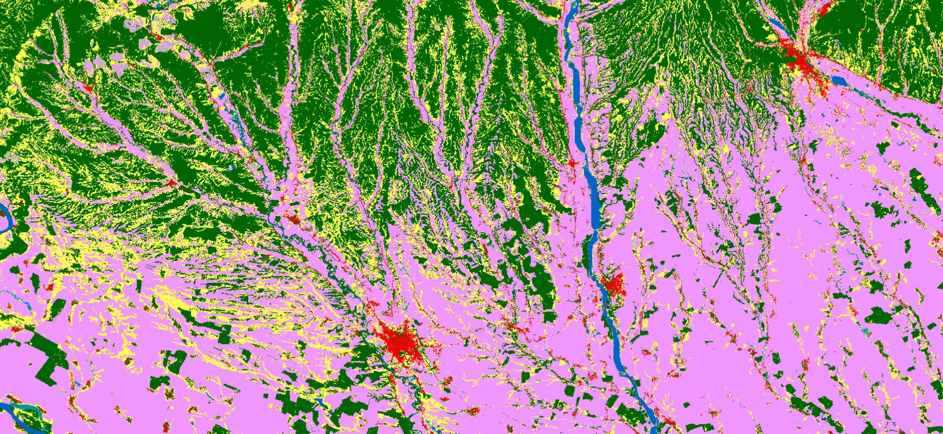


**BILINEAR** - [bilinear interpolation](https://en.wikipedia.org/wiki/Bilinear_interpolation)
**BICUBIC** - [bicubic interpolation](https://en.wikipedia.org/wiki/Bicubic_interpolation) | **NEAREST** | | downsampling | As above except when the resolution is lower. | **NEAREST** - [nearest neighbour interpolation](https://en.wikipedia.org/wiki/Nearest-neighbor_interpolation)
**BILINEAR** - [bilinear interpolation](https://en.wikipedia.org/wiki/Bilinear_interpolation)
**BICUBIC** - [bicubic interpolation](https://en.wikipedia.org/wiki/Bicubic_interpolation) | **NEAREST** | | egm | An option to add geoid heights from an earth gravitational model to the orthometric heights in which case the returned values represent ellipsoidal heights relative to the WGS84 ellipsoid.

For Mapzen's DEM, we use [EGM96](https://en.wikipedia.org/wiki/Earth_Gravitational_Model#EGM96), and for Copernicus DEMs, we use [EGM2008](https://en.wikipedia.org/wiki/Earth_Gravitational_Model#EGM2008). | **TRUE** - returned values are ellipsoid heights
**FALSE** - returned values are orthometric heights | **FALSE** | | clampNegative | **Mapzen DEM** specific option. It replaces negative orthometric heights with 0. Useful for removing ocean bathymetry, for example.

*Note: If `clampNegative:true` and `egm: true` it is still possible to have negative output values. This is because the egm offset can be negative and it is applied after clampNegative.* | **TRUE** - negative orthometric heights are replaced with 0.
**FALSE** - no changes. | **FALSE** | ### Available Bands and Data Information in this chapter is useful when defining [`input` object](https://docs.planet.com/develop/evalscripts/functions.md#input-object-properties) in evalscript. A string listed in the column **Name** can be an element of the `input.bands` array in your evalscript. | Property name | Description | Resolution | | ------------- | --------------------------------------------------------------------------------------------------- | ---------------------------------------------------------------------------------------------------------------------------------------------------------------- | | DEM | Heights in meters | Various, depending on the datasource used for the generation of the DEM, [see](https://github.com/tilezen/joerd/blob/master/docs/images/footprints-preview.png). | | dataMask | The mask of data/no data pixels ([more](https://docs.planet.com/develop/evalscripts.md#data-mask)). | N/A\* | \*dataMask has no source resolution as it is calculated for each output pixel. ### Units The data values for each band in your custom script are presented in the units as specified here. In case more than one unit is available for a given band, you may optionally set the value of `input.units` in your evalscript `setup` function to one of the values in the `Units Value` column. Doing so will present data in that unit. The `units` parameter combines the physical quantity and corresponding units of measurement values. As such, some names more closely resemble physical quantities, others resemble units of measurement. The `Source Format` specifies how and with what precision the digital numbers (`DN`) from which the unit is derived are encoded. Bands requested in `DN` units contain exactly the pixel values of the source data. Note that resampling may produce interpolated values. `DN` is also used whenever a band is derived computationally (like dataMask); such bands can be identified by having `DN` units and `N/A` source format. `DN` values are typically not offered if they do not simply represent any physical quantity, in particular, when `DN` values require source-specific (i.e. non-global) conversion to physical quantities. Values in non-`DN` units are computed from the source (`DN`) values with at least float32 precision. Note that the conversion might be nonlinear, therefore the full value range and quantization step size of such a band can be hard to predict. Band values in evalscripts always behave as floating point numbers, regardless of the actual precision. The `Typical Range` indicates what values are common for a given band and unit, however outliers can be expected. For DEM, `DN` (digital numbers) are the default and only unit. `DN` values equal elevation. | Band | Physical Quantity (units) | Units Value | Source Format | Typical Range | | -------- | ------------------------- | ----------- | --------------------- | ------------------------- | | DEM | Height (meters) | METERS | INT16 or FLOAT32 \[1] | \[2] | | dataMask | N/A | DN | N/A | 0 - no data
1 - data | \[1]: Copernicus DEM is always FLOAT32. MAPZEN is typically INT16 but occasionally FLOAT32. \[2]: MAPZEN includes bathymetry data while Copernicus DEM does not. As such, MAPZEN values can extend to -11000 (Mariana Trench), while Copernicus DEM values are typically positive. The highest point is of course Mount Everest at slightly less than +9000 meters. ### Scene Object The [evalscript evaluatePixel scene object](https://docs.planet.com/develop/evalscripts/functions.md#evaluatepixel) is not returned/is null when requesting DEM. ### Collection specific constraints DEM values are in meters and can be negative for areas which lie below sea level (for example, ocean areas or much of the Netherlands). When requesting a DEM a simple way to mitigate this is to set the output format in your evalscript to **`sampleType: SampleType.FLOAT32`** or **`sampleType: SampleType.INT16`** if this provides sufficient precision for your use. More about output formats can be found [here](https://docs.planet.com/develop/evalscripts/functions.md#sampletype). For output formats `sampleType: SampleType.UINT8` and `sampleType: SampleType.UINT16` be careful as negative values can be misinterpreted due to signedness issues as well as potential problems due to [integer overflow](https://en.wikipedia.org/wiki/Integer_overflow). For example: * `sampleType: SampleType.UINT8` - a height of 256 meters will be encoded as 0 in such a file due to overflow. A height of -1 meter will be encoded as 255. * `sampleType: SampleType.UINT16`- a height of -15 meters for instance will be encoded as 65520. One way to handle this adjustment is to ensure there are no negative values in the output by adding a constant to DEM values, for example, 12000 (the minimum value in DEM is not smaller than -11000 m). If you need actual DEM values (i.e. heights), the constant 12000 must be subtracted from the output values outside. ``` //VERSION=3 function setup() { return { input: ['DEM'], output: { id: 'default', bands: 1, sampleType: SampleType.UINT16, }, }; } function evaluatePixel(sample) { return [sample.DEM + 12000]; } ``` --- Copy for LLM[View as Markdown](https://docs.planet.com/data/public-data/other-datasets/dem/examples/) # Digital Elevation Model (DEM) Examples The following examples are CURL requests and can be run from the command line or terminal. In addition, you can copy and paste these examples into [Request Builder](https://insights.planet.com/analyze/requests-builder/). You can translate the requests into other programming languages in the Request Builder app. To request data using any of the request below, you will need to replace the string `` with your access token. Your access token will look something like this: ``` ayJhbGciOiJSUzI1NiJ9.ayJzdWIiOiI0MmYwODZjCy1kMzI3LTRlOTMtYWMxNS00ODAwOGFiZjI0YjIiLCJhdWQiOiJlY2I1MGM1Zi1i MWM1LTQ3ZTgtYWE4NC0zZTU4NzJlM2I2MTEiLCJqdGkiOiI5MzYxMWE4ODEyNTM4Y2M0MmU0NDJjYjUyMTY0YmJlNyIsImV4cCI6MTU1N TQyMzk3MiwibmFtZSI6ImFuamEudnJlY2tvQHNpbmVyZ2lzZS5jb20iLCJlbWFpbCI6ImFuamEudnJlY2tvQHNpbmVyZ2lzZS5jb20iLC JzaWQiOiIzZjVjZDVkNS04MjRiLTQ3ZjYtODgwNy0wNDMyNWY4ODQxZmQifQ.U7FPOy_2jlEOFxXSjyN5KEdBROna3-Dyec0feShIbUOY 1p9lEXdNaMmR5euiINi2RXDayX9Kr47CuSTsvq1zHFvZs1YgkFr1iH6kDuX-t_-wfWpqu5oPjoPVKZ4Rj0Ms_dxAUTQFTXR0rlbLuO-KS gnaeLVb5iiv_qY3Ctq2XKdIRcFRQLFziFcP4yZJl-NZMlwzsiiwjakcpYpI5jSYAdU2hpZLHRzceseeZt5YfZOe5Px1kZXro9Nd0L2GPC -qzOXw_V1saMGFa2ov8qV6Dvk92iv2SDDdGhOdII_JOf8XkK4E3g2z0EEFdWhG9F4Iky4ukNsqBPgE8LRb31s0hg ``` and can be obtained as described in the [Authentication chapter](https://docs.planet.com/develop/authentication.md). ## Copernicus DEM 30 image (png) ``` curl -X POST \ https://services.sentinel-hub.com/process/v1 \ -H 'Authorization: Bearer ' \ -H 'content-type: multipart/form-data' \ -F 'request={ "input": { "bounds": { "properties": { "crs": "http://www.opengis.net/def/crs/OGC/1.3/CRS84" }, "bbox": [ 13.822174072265625, 45.85080395917834, 14.55963134765625, 46.29191774991382 ] }, "data": [{ "type": "dem", "dataFilter": { "demInstance": "COPERNICUS_30" }, "processing": { "upsampling": "BILINEAR", "downsampling": "BILINEAR" } }] }, "output": { "width": 512, "height": 512, "responses": [{ "identifier": "default", "format": { "type": "image/png" } }] } }' \ -F 'evalscript=//VERSION=3 function setup() { return { input: ["DEM"], output: { bands: 1 } } } function evaluatePixel(sample) { return [sample.DEM/1000] }' ``` ## Mapzen DEM image (png) ``` curl -X POST \ https://services-uswest2.sentinel-hub.com/process/v1 \ -H 'Authorization: Bearer ' \ -H 'content-type: multipart/form-data' \ -F 'request={ "input": { "bounds": { "properties": { "crs": "http://www.opengis.net/def/crs/OGC/1.3/CRS84" }, "bbox": [ 13.822174072265625, 45.85080395917834, 14.55963134765625, 46.29191774991382 ] }, "data": [{ "type": "dem", "dataFilter": { "demInstance": "MAPZEN" }, "processing": { "upsampling": "BILINEAR", "downsampling": "BILINEAR" } }] }, "output": { "width": 512, "height": 512, "responses": [{ "identifier": "default", "format": { "type": "image/png" } }] } }' \ -F 'evalscript=//VERSION=3 function setup() { return { input: ["DEM"], output: { bands: 1 } } } function evaluatePixel(sample) { return [sample.DEM/1000] }' ``` ## Copernicus DEM 30, 0.0003° (\~33m) resolution (tiff) ``` curl -X POST \ https://services.sentinel-hub.com/process/v1 \ -H 'Authorization: Bearer ' \ -H 'content-type: multipart/form-data' \ -F 'request={ "input": { "bounds": { "properties": { "crs": "http://www.opengis.net/def/crs/OGC/1.3/CRS84" }, "bbox": [ 13.822174072265625, 45.85080395917834, 14.55963134765625, 46.29191774991382 ] }, "data": [{ "type": "dem", "dataFilter": { "demInstance": "COPERNICUS_30" }, "processing": { "upsampling": "BILINEAR", "downsampling": "BILINEAR" } }] }, "output": { "resx": 0.0003, "resy": 0.0003, "responses": [{ "identifier": "default", "format": { "type": "image/tiff" } }] } }' \ -F 'evalscript=//VERSION=3 function setup() { return { input: ["DEM"], output: { bands: 1 } } } function evaluatePixel(sample) { return [sample.DEM/1000] }' ``` ## Copernicus DEM 90 values, orthometric heights (tif) ``` curl -X POST \ https://services.sentinel-hub.com/process/v1 \ -H 'Authorization: Bearer ' \ -H 'content-type: multipart/form-data' \ -F 'request={ "input": { "bounds": { "properties": { "crs": "http://www.opengis.net/def/crs/OGC/1.3/CRS84" }, "bbox": [ 13.822174072265625, 45.85080395917834, 14.55963134765625, 46.29191774991382 ] }, "data": [{ "type": "dem", "dataFilter": { "demInstance": "COPERNICUS_90" }, "processing": { "upsampling": "BILINEAR", "downsampling": "BILINEAR" } }] }, "output": { "width": 512, "height": 512, "responses": [{ "identifier": "default", "format": { "type": "image/tiff" } }] } }' \ -F 'evalscript=//VERSION=3 function setup() { return { input: ["DEM"], output: { id: "default", bands: 1, sampleType: SampleType.FLOAT32 } } } function evaluatePixel(sample) { return [sample.DEM] }' ``` ## Copernicus DEM 90 values, ellipsoidal heights (tif) ``` curl -X POST \ https://services.sentinel-hub.com/process/v1 \ -H 'Authorization: Bearer ' \ -H 'content-type: multipart/form-data' \ -F 'request={ "input": { "bounds": { "properties": { "crs": "http://www.opengis.net/def/crs/OGC/1.3/CRS84" }, "bbox": [ 13.822174072265625, 45.85080395917834, 14.55963134765625, 46.29191774991382 ] }, "data": [{ "type": "dem", "dataFilter": { "demInstance": "COPERNICUS_90" }, "processing": { "egm": true, "upsampling": "BILINEAR", "downsampling": "BILINEAR" } }] }, "output": { "width": 512, "height": 512, "responses": [{ "identifier": "default", "format": { "type": "image/tiff" } }] } }' \ -F 'evalscript=//VERSION=3 function setup() { return { input: ["DEM"], output: { id: "default", bands: 1, sampleType: SampleType.FLOAT32 } } } function evaluatePixel(sample) { return [sample.DEM] }' ``` ## Copernicus DEM 90 image at sea level (png) ``` curl -X POST \ https://services.sentinel-hub.com/process/v1 \ -H 'Authorization: Bearer ' \ -H 'content-type: multipart/form-data' \ -F 'request={ "input": { "bounds": { "properties": { "crs": "http://www.opengis.net/def/crs/OGC/1.3/CRS84" }, "bbox": [ 10.082016, 42.625876, 10.496063, 42.927268 ] }, "data": [{ "type": "dem", "dataFilter": { "demInstance": "COPERNICUS_90" }, "processing": { "upsampling": "BILINEAR", "downsampling": "BILINEAR" } }] }, "output": { "width": 512, "height": 512, "responses": [{ "identifier": "default", "format": { "type": "image/png" } }] } }' \ -F 'evalscript=//VERSION=3 function setup() { return { input: ["DEM"], output: { bands: 3 } } } function evaluatePixel(sample) { if (sample.DEM > 0) { return [0, sample.DEM / 1000, 0] } else { return [0, 0, -sample.DEM / 100] } }' ``` ## Mapzen DEM image at sea level, clampNegatives (png) ``` curl -X POST \ https://services-uswest2.sentinel-hub.com/process/v1 \ -H 'Authorization: Bearer ' \ -H 'content-type: multipart/form-data' \ -F 'request={ "input": { "bounds": { "properties": { "crs": "http://www.opengis.net/def/crs/OGC/1.3/CRS84" }, "bbox": [ 10.082016, 42.625876, 10.496063, 42.927268 ] }, "data": [{ "type": "dem", "dataFilter": { "demInstance": "MAPZEN" }, "processing": { "clampNegative": true, "upsampling": "BILINEAR", "downsampling": "BILINEAR" } }] }, "output": { "width": 512, "height": 512, "responses": [{ "identifier": "default", "format": { "type": "image/png" } }] } }' \ -F 'evalscript=//VERSION=3 function setup() { return { input: ["DEM"], output: { bands: 1 } } } function evaluatePixel(sample) { return [sample.DEM / 1000] }' ``` ## Mapzen DEM values at sea level, orthometric heights, clampNegatives (tif) ``` curl -X POST \ https://services-uswest2.sentinel-hub.com/process/v1 \ -H 'Authorization: Bearer ' \ -H 'content-type: multipart/form-data' \ -F 'request={ "input": { "bounds": { "properties": { "crs": "http://www.opengis.net/def/crs/OGC/1.3/CRS84" }, "bbox": [ 10.082016, 42.625876, 10.496063, 42.927268 ] }, "data": [{ "type": "dem", "dataFilter": { "demInstance": "MAPZEN" }, "processing": { "egm": false, "clampNegative": true, "upsampling": "BILINEAR", "downsampling": "BILINEAR" } }] }, "output": { "width": 512, "height": 512, "responses": [{ "identifier": "default", "format": { "type": "image/tiff" } }] } }' \ -F 'evalscript=//VERSION=3 function setup() { return { input: ["DEM"], output: { id: "default", bands: 1, sampleType: SampleType.FLOAT32 } } } function evaluatePixel(sample) { return [sample.DEM] }' ``` ## Mapzen DEM values at sea level, orthometric heights including negative values (tif) ``` curl -X POST \ https://services-uswest2.sentinel-hub.com/process/v1 \ -H 'Authorization: Bearer ' \ -H 'content-type: multipart/form-data' \ -F 'request={ "input": { "bounds": { "properties": { "crs": "http://www.opengis.net/def/crs/OGC/1.3/CRS84" }, "bbox": [ 10.082016, 42.625876, 10.496063, 42.927268 ] }, "data": [{ "type": "dem", "dataFilter": { "demInstance": "MAPZEN" }, "processing": { "clampNegative": false, "upsampling": "BILINEAR", "downsampling": "BILINEAR" } }] }, "output": { "width": 512, "height": 512, "responses": [{ "identifier": "default", "format": { "type": "image/tiff" } }] } }' \ -F 'evalscript=//VERSION=3 function setup() { return { input: ["DEM"], output: { id: "default", bands: 1, sampleType: SampleType.FLOAT32 } } } function evaluatePixel(sample) { return [sample.DEM] }' ``` --- Copy for LLM[View as Markdown](https://docs.planet.com/data/public-data/other-datasets/esa-worldcover/) # ESA WorldCover ![Header Thumbnail](/data/public-data/other-datasets/south-romania.webp) The ESA WorldCover product provides global land cover maps for 2020 and 2021. By combining the strengths of both Sentinel-1 (SAR) and Sentinel-2 (optical), it achieves a more consistent global result than optical-only products. The 2020 version (v100) and 2021 version (v200) use slightly different algorithms, so users should exercise caution when performing direct change detection between the two years. ## Data Availability & Collections The WorldCover map is accessible via the [Planet Insights Platform](https://insights.planet.com/) as a Bring Your Own COG (BYOC) collection. * **Collection ID**: `0b940c63-45dd-4e6b-8019-c3660b81b884` * **Update Frequency**: Annual (2020 and 2021 currently available). ## Basic Facts | Property | Value | | ----------------------- | --------------------------------------------------------- | | **Sensor** | Sentinel-1 (C-SAR) and Sentinel-2 (MSI) | | **Spatial Resolution** | 10 m | | **Geographic Coverage** | Global | | **Coordinate System** | WGS 84 (EPSG:4326) | | **Data Format** | Cloud Optimized GeoTIFF (COG) | | **Temporal Coverage** | 2020, 2021 | | **License** | [CC-BY 4.0](https://creativecommons.org/licenses/by/4.0/) | | **Provider** | **Planet** | ## Band Information The collection contains the main classification map and a multi-band quality layer. | Name | Description | | ---------------- | ---------------------------------------------------------------------------------- | | **Map** | Main discrete classification according to FAO LCCS scheme (11 classes). | | **InputQuality** | 3-band layer indicating the number and quality of S1 and S2 inputs used per pixel. | ## Class Definitions The `Map` band contains the following 11 land cover classes: | Value | Label | Color | | ------- | ------------------------ | --------- | | **10** | Tree cover | `#006400` | | **20** | Shrubland | `#ffbb22` | | **30** | Grassland | `#ffff4c` | | **40** | Cropland | `#f096ff` | | **50** | Built-up | `#fa0000` | | **60** | Bare / sparse vegetation | `#b4b4b4` | | **70** | Snow and ice | `#f0f0f0` | | **80** | Permanent water bodies | `#0064c8` | | **90** | Herbaceous wetland | `#0096a0` | | **95** | Mangroves | `#00cf75` | | **100** | Moss and lichen | `#fae6a0` | ## Accessing the Data ### Planet Insights Platform API To access the data programmatically: * **Endpoint**: `services.sentinel-hub.com` * **Collection Type**: `byoc-0b940c63-45dd-4e6b-8019-c3660b81b884` ### Visualization Script (Evalscript) Use the following script to visualize the WorldCover map with its standard color palette: ``` // VERSION=3 // ESA WorldCover Visualization Script const colormap = [ [10, 0x006400], // Tree cover [20, 0xffbb22], // Shrubland [30, 0xffff4c], // Grassland [40, 0xf096ff], // Cropland [50, 0xfa0000], // Built-up [60, 0xb4b4b4], // Bare / sparse vegetation [70, 0xf0f0f0], // Snow and ice [80, 0x0064c8], // Permanent water bodies [90, 0x0096a0], // Herbaceous wetland [95, 0x00cf75], // Mangroves [100, 0xfae6a0], // Moss and lichen ]; const visualizer = new ColorMapVisualizer(colormap); function setup() { return { input: ['Map', 'dataMask'], output: { bands: 3 }, }; } function evaluatePixel(samples) { return visualizer.process(samples.Map); } ``` ## Attribution © ESA WorldCover project / Contains modified Copernicus Sentinel data (2020/2021) processed by ESA WorldCover consortium. --- Copy for LLM[View as Markdown](https://docs.planet.com/data/public-data/other-datasets/impact-observatory-lulc-map/) # 10m Annual Land Use Land Cover (9-class) ![Header Thumbnail](/data/public-data/other-datasets/io-lulc-ganges-delta.webp) The **10m Annual Land Use Land Cover (9-class)** dataset is a global map produced by **Impact Observatory**, **Microsoft**, and **Esri**. It provides a year-by-year snapshot of global land cover at a 10-meter resolution, derived from ESA Sentinel-2 imagery using a deep learning AI model. This dataset is particularly valuable for monitoring urbanization, deforestation, and agricultural expansion over time. ## Data Availability & Collections The dataset is organized as a "Bring Your Own COG" (BYOC) collection within the [Planet Insights Platform](https://insights.planet.com/). Each pixel represents the most likely land cover class for the given year. * **Collection ID**: `0ed26381-7344-4281-b180-66f3da521f75` * **Update Frequency**: The map is updated annually following the completion of the calendar year. ## Basic Facts | Property | Value | | ---------------------- | --------------------------------------------------------- | | **Sensor** | MultiSpectral Instrument (MSI) from Sentinel-2 | | **Spatial Resolution** | 10 m | | **Coordinate System** | UTM (aligned to Sentinel-2 tiling grid) | | **Data Format** | Cloud Optimized GeoTIFF (COG) | | **Temporal Coverage** | 2017 – 2023 (Updated annually) | | **License** | [CC-BY 4.0](https://creativecommons.org/licenses/by/4.0/) | | **Provider** | **Planet** | ## Class Definitions The product consists of a single band named `lulc`. Each pixel contains an integer value from 1 to 11. Note that values 3 and 6 are not used in this 9-class schema. | Value | Label | Color | | ------ | ---------------------- | --------- | | **1** | **Water** | `#419bdf` | | **2** | **Trees** | `#397d49` | | **4** | **Flooded Vegetation** | `#7a87c6` | | **5** | **Crops** | `#e49635` | | **7** | **Built Area** | `#c4281b` | | **8** | **Bare Ground** | `#a59b8f` | | **9** | **Snow/Ice** | `#a8ebff` | | **10** | **Clouds** | `#616161` | | **11** | **Rangeland** | `#e3e2c3` | ## Accessing the Data ### AWS S3 Access The data is hosted in the AWS `us-west-2` region. You can browse the directory structure using the AWS CLI: ``` aws s3 ls --no-sign-request s3://io-10m-annual-lulc/ ``` ### Planet Insights Platform API To access the data programmatically via the [Planet Insights Platform](https://insights.planet.com/): * Endpoint: `services.sentinel-hub.com` * Collection Type: `byoc-0ed26381-7344-4281-b180-66f3da521f75` ## Visualization Script (Evalscript) To view the land cover map with the standard classification colors, use the following [Evalscript](https://docs.planet.com/develop/evalscripts.md) in your request: ``` // VERSION=3 // Impact Observatory 10m LULC Visualizer const colormap = [ [1, 0x419bdf], // Water [2, 0x397d49], // Trees [4, 0x7a87c6], // Flooded Vegetation [5, 0xe49635], // Crops [7, 0xc4281b], // Built Area [8, 0xa59b8f], // Bare Ground [9, 0xa8ebff], // Snow/Ice [10, 0x616161], // Clouds [11, 0xe3e2c3], // Rangeland ]; const visualizer = new ColorMapVisualizer(colormap); function setup() { return { input: ['lulc', 'dataMask'], output: { bands: 3 }, }; } function evaluatePixel(samples) { return visualizer.process(samples.lulc); } ``` ## Attribution This dataset is collaboratively produced by [Impact Observatory](https://www.impactobservatory.com/maps-for-good/), Microsoft, and Esri. It contains modified Copernicus Sentinel data processed by these partners. --- Copy for LLM[View as Markdown](https://docs.planet.com/data/public-data/other-datasets/sentinel-s2-l2a-mosaic-120/) # Sentinel-2 L2A 120m Mosaic ![Header Thumbnail](/data/public-data/other-datasets/world-mosaic-2020.webp) The Sentinel-2 L2A 120m mosaic is a derived product that provides the "best pixel" values for 10-daily periods. It is modeled by removing cloudy pixels and performing linear interpolation among the remaining valid observations. While designed to be cloud-free, some clouds may remain in regions with persistent, lengthy cloudy periods. ## Data Availability & Collections The mosaic is split into annual collections with different band configurations. * 2020 Collection: Contains 12 spectral bands and 1 quality mask. * **Collection ID**: `484d8dbb-9e3e-41f2-b96b-35189d3ae37f` * 2019 Collection: Contains 6 spectral bands. * **Collection ID**: `0074520d-bcf5-4811-8f6f-afd946e77695` ## Basic Facts | Property | Value | | ---------------------- | --------------------------------------------------------- | | **Sensor** | MultiSpectral Instrument (MSI) from Sentinel-2 | | **Spatial Resolution** | 120 m | | **Coordinate System** | UTM | | **Data Format** | Cloud Optimized GeoTIFF (COG) | | **Temporal Coverage** | 2019, 2020 (Annual updates) | | **License** | [CC-BY 4.0](https://creativecommons.org/licenses/by/4.0/) | | **Provider** | **Planet** | ## Band Information (2019 Product) The 2019 mosaic includes the following 6 bands, typically provided in Digital Numbers (DN) ranging from 0 to 10,000. | Name | Description | Resolution | | ---- | ----------- | ---------- | | B02 | Blue | 120 m | | B03 | Green | 120 m | | B04 | Red | 120 m | | B08 | NIR | 120 m | | B11 | SWIR 1 | 120 m | | B12 | SWIR 2 | 120 m | ## Quality Mask (QM) The `QM` band is essential for identifying the reliability of the interpolated data. It is recommended to filter data where `QM != 0`. | Value | Meaning | Description | | ----- | -------------------- | -------------------------------------------------------------- | | 0 | No Data | Areas where no valid observations were found. | | 1 | Interpolation Passed | Areas where the interpolation successfully finished. | | 2 | Artificially Raised | DN values raised from 0 to 1 to avoid confusion with NO\_DATA. | | 3 | Interpolation Failed | Detected persistent clouds; values set to maximum (10,000). | ## Accessing the Data ### AWS S3 Access The data is hosted on AWS in the `eu-central-1` region. You can list objects using the AWS CLI without an account: ``` aws s3 ls --no-sign-request s3://sentinel-s2-l2a-mosaic-120/2019/ ``` Path Structure: `[year]/[month]/[day]/[UTM_code][latitude_band]/` ### Planet Insights Platform API To access the data programmatically via the [Planet Insights Platform](https://insights.planet.com/): * Endpoint: `services.sentinel-hub.com` * Collection Type: `byoc-[Collection_ID]` ## Band Information (2020 Product) The 2020 mosaic contains the full spectral range of Sentinel-2. | Name | Description | Resolution | | ----------- | ---------------- | ---------- | | **B01** | Coastal aerosol | 120 m | | **B02** | Blue | 120 m | | **B03** | Green | 120 m | | **B04** | Red | 120 m | | **B05-B07** | Red Edge | 120 m | | **B08/B8A** | NIR / Narrow NIR | 120 m | | **B09** | Water Vapour | 120 m | | **B11/B12** | SWIR 1 / SWIR 2 | 120 m | | **QM** | Quality Mask | 120 m | ### Custom Scripts: Interpolated Time-Series For users wanting to recreate or customize this mosaic, an **Interpolated Time-series** script is available. This script: 1. Defines a start and end date (for example, a full year). 2. Splits the timeframe into equal 10-daily intervals. 3. Applies cloud masking using `CLM` and `CLP` bands. 4. Performs linear interpolation to fill gaps caused by cloud cover. **Example Evalscript Snippet:** ``` // VERSION=3 // Basic linear interpolation logic used for the 120m mosaic function linearInterpolation(x, x0, y0, x1, y1) { var a = (y1 - y0) / (x1 - x0); var b = -a * x0 + y0; return a * x + b; } ``` ## Attribution Contains modified Copernicus Sentinel data \[Year] processed by Sentinel Hub. For citations, use: Sentinel-2 L2A 120m Mosaic was accessed on \[DATE] from . --- Copy for LLM[View as Markdown](https://docs.planet.com/data/public-data/usgs-nasa/) # USGS & NASA Imagery [![](/data/public-data/harmonized-landsat-sentinel/thumbnail.webp)](https://docs.planet.com/data/public-data/usgs-nasa/harmonized-landsat-sentinel.md) ### [Harmonized Landsat Sentinel](https://docs.planet.com/data/public-data/usgs-nasa/harmonized-landsat-sentinel.md) [Use Processing API to access Harmonized Landsat Sentinel data with 13 optical and 2 thermal bands.](https://docs.planet.com/data/public-data/usgs-nasa/harmonized-landsat-sentinel.md) [![](/data/public-data/landsat-4-5-tm/thumbnail.webp)](https://docs.planet.com/data/public-data/usgs-nasa/landsat-4-5-tm.md) ### [Landsat 4-5 TM L1 & L2](https://docs.planet.com/data/public-data/usgs-nasa/landsat-4-5-tm.md) [Use Processing API to access Landsat 4–5 Thematic Mapper (TM) Level 1 and Level 2 data, including optical, thermal, and surface reflectance products.](https://docs.planet.com/data/public-data/usgs-nasa/landsat-4-5-tm.md) [![](/data/public-data/landsat-7-etm/thumbnail.webp)](https://docs.planet.com/data/public-data/usgs-nasa/landsat-7-etm.md) ### [Landsat 7 ETM+ L1 & L2](https://docs.planet.com/data/public-data/usgs-nasa/landsat-7-etm.md) [Use Processing API to access Landsat 7 Enhanced Thematic Mapper Plus (ETM+) Level 1 and Level 2 data, including optical, thermal, and surface reflectance products.](https://docs.planet.com/data/public-data/usgs-nasa/landsat-7-etm.md) [![](/data/public-data/landsat-8-9/thumbnail.webp)](https://docs.planet.com/data/public-data/usgs-nasa/landsat-8-9.md) ### [Landsat 8-9 L1 & L2](https://docs.planet.com/data/public-data/usgs-nasa/landsat-8-9.md) [Use Processing API to access Landsat 8–9 Level 1 and Level 2 data, including optical, thermal, and surface reflectance products.](https://docs.planet.com/data/public-data/usgs-nasa/landsat-8-9.md) --- Copy for LLM[View as Markdown](https://docs.planet.com/data/public-data/usgs-nasa/harmonized-landsat-sentinel/) # Harmonized Landsat Sentinel ![Header Thumbnail](/data/public-data/harmonized-landsat-sentinel/thumbnail.webp) Harmonized Landsat Sentinel is a NASA initiative to produce a Virtual Constellation of surface reflectance (SR) data from the Operational Land Imager (OLI) and Multi-Spectral Instrument (MSI) aboard the Landsat 8-9 and Sentinel-2 remote sensing satellites, respectively. The combined measurement enables global observations of the land every 2–3 days. Input products are Landsat 8-9 Collection 2 Level 1 top-of-atmosphere reflectance and Sentinel-2 L1C top-of-atmosphere reflectance, which NASA radiometrically harmonizes to the maximum extent, resamples to common 30-meter resolution, and grids using the Sentinel-2 Military Grid Reference System (MGRS) UTM grid. Because of this, the products are different from Landsat 8-9 Collection 2 Level 2 surface reflectance and Sentinel-2 L2A surface reflectance. Learn more about the data [here](https://lpdaac.usgs.gov/data/get-started-data/collection-overview/missions/harmonized-landsat-sentinel-2-hls-overview/). ### Basic Facts | Property | Info | | ------------------------ | ------------------------------------------------------------------------------------------------ | | **Spatial resolution** | 30 m | | **Sensor** | Operational Land Imager for Landsat 8-9, and MultiSpectral Instrument for Sentinel-2 satellites. | | **Revisit time** | 2-3 days | | **Spatial coverage** | Whole globe | | **Data availability** | Landsat 8-9 since April 2013, Sentinel-2 since November 2015. | | **Common usage/purpose** | Vegetation monitoring, land use, land cover maps and monitoring of changes. | ## Accessing Data To access data you need to send a POST request to our `process` API. The requested data will be returned as the response to your request. Each POST request can be tailored to get you exactly the data you require. To do this requires setting various parameters which depend on the collection you are querying. This chapter will help you understand the parameters for HLS data. For an overview of all API parameters see the [API Reference](https://docs.planet.com/develop/apis.md). ### Endpoint Locations | Service | Notes | | ------------------------------------- | ------------------------------------------------------------- | | services-uswest2.sentinel-hub.com/api | Landsat 8-9 since April 2013, Sentinel-2 since November 2015. | ### Data type identifier: `hls` Use `hls` as the value of the `input.data.type parameter` in your API requests. This is mandatory and will ensure you get HLS data. ### Filtering Options This chapter will explain the `input.data.dataFilter` object of the `process` API. #### `mosaickingOrder` Sets the order of overlapping tiles from which the output result is mosaicked. Note that tiles will in most cases come from the same orbit/acquisition. The tiling is done by NASA for easier distribution. | Value | Description | Notes | | --------------- | ------------------------------------------------------------------------- | ------------------------------------------------------------------------------------------------------------- | | **mostRecent** | (default) The pixel will be selected from the most recently acquired tile | | | **leastRecent** | similar to **mostRecent** but in reverse order | | | **leastCC** | The pixel is selected from the tile with the lowest cloud coverage | This information is estimated per tile (each covering about 31,100 sq. km) so local cloud coverage may differ | #### `maxCloudCoverage` Sets the upper limit for cloud coverage in percent based on the precomputed cloud coverage estimate for each tile as present in the tile metadata. Satellite data will therefore not be retrieved for tiles with a higher cloud coverage estimate. For example, by setting the value to `20`, only tiles with at most 20% cloud coverage will be used. Note that this parameter is set per tile and might not be directly applicable to the chosen area of interest. #### `constellation` Selects constellation. By default, both constellations are selected. Note that for any type of data mosaicking, for requests containing bands which are present in only one constellation (e.g. `RedEdge1`), it is highly recommended (but not strictly necessary) to set the corresponding `constellation` parameter. Otherwise, your request may fail as the band is not guaranteed to be present for all data being mosaicked. | Value | Description | | ------------ | ------------------------------ | | **SENTINEL** | selects only Sentinel products | | **LANDSAT** | selects only Landsat products | ### Processing Options This chapter will explain the `input.data.processing` object of the `process` API. | Parameter | Description | | ------------ | -------------------------------------------------------------------------------------------------------------- | | upsampling | [The same as for S2L1C.](https://docs.planet.com/data/public-data/copernicus/sentinel-2.md#processing-options) | | downsampling | [The same as for S2L1C.](https://docs.planet.com/data/public-data/copernicus/sentinel-2.md#processing-options) | ### Available Bands and Data Information in this chapter is useful when defining [`input` object](https://docs.planet.com/develop/evalscripts/functions.md#input-object-properties) in evalscript. Any string listed in the column **Name** can be an element of the `input.bands` array in your evalscript. | Name | Description | Resolution | Constellation | | ---------------- | --------------------------------------------------------------------------------------------------- | ---------- | ------------- | | CoastalAerosol | Coastal Aerosol - band 1 from Landsat and Sentinel | 30 m | Both | | Blue | Blue - band 2 from both | 30 m | Both | | Green | Green - band 3 from both | 30 m | Both | | Red | Red - band 4 from both | 30 m | Both | | RedEdge1 | Red-Edge 1 - band 5 from Sentinel | 30 m | Sentinel | | RedEdge2 | Red-Edge 2 - band 6 from Sentinel | 30 m | Sentinel | | RedEdge3 | Red-Edge 3 - band 7 from Sentinel | 30 m | Sentinel | | NIR\_Broad | NIR Broad - band 8 from Sentinel | 30 m | Sentinel | | NIR\_Narrow | NIR Narrow - band 5 from Landsat and 8A from Sentinel | 30 m | Both | | SWIR1 | SWIR 1 - band 6 from Landsat and 11 from Sentinel | 30 m | Both | | SWIR2 | SWIR 2 - band 7 from Landsat and 12 from Sentinel | 30 m | Both | | WaterVapor | Water Vapor - band 9 from Sentinel | 30 m | Sentinel | | Cirrus | Cirrus - band 9 from Landsat and 10 from Sentinel | 30 m | Both | | ThermalInfrared1 | Thermal Infrared 1 - band 10 from Landsat | 30 m | Landsat | | ThermalInfrared2 | Thermal Infrared 2 - band 11 from Landsat | 30 m | Landsat | | QA | Quality Assessment band (QA) | 30 m | Both | | VAA | View (sensor) Azimuth Angle | 30 m | Both | | VZA | View (sensor) Zenith Angle | 30 m | Both | | SAA | Sun Azimuth Angle | 30 m | Both | | SZA | Sun Zenith Angle | 30 m | Both | | dataMask | The mask of data/no data pixels ([more](https://docs.planet.com/develop/evalscripts.md#data-mask)). | N/A \[1] | Both | \[1]: dataMask has no source resolution as it is calculated for each output pixel. For more info about the bands, check [HLS user guide](https://lpdaac.usgs.gov/documents/1698/HLS_User_Guide_V2.pdf). ### Units The data values for each band in your custom script are presented in the units as specified here. In case more than one unit is available for a given band, you may optionally set the value of `input.units` in your evalscript `setup` function to one of the values in the `Units Value` column. Doing so will present data in that unit. The `units` parameter combines the physical quantity and corresponding units of measurement values. As such, some names more closely resemble physical quantities, others resemble units of measurement. The `Source Format` specifies how and with what precision the digital numbers (`DN`) from which the unit is derived are encoded. Bands requested in `DN` units contain exactly the pixel values of the source data. Note that resampling may produce interpolated values. `DN` is also used whenever a band is derived computationally (like dataMask); such bands can be identified by having `DN` units and `N/A` source format. `DN` values are typically not offered if they do not simply represent any physical quantity, in particular, when `DN` values require source-specific (i.e. non-global) conversion to physical quantities. Values in non-`DN` units are computed from the source (`DN`) values with at least float32 precision. Note that the conversion might be nonlinear, therefore the full value range and quantization step size of such a band can be hard to predict. Band values in evalscripts always behave as floating point numbers, regardless of the actual precision. The `Typical Range` indicates what values are common for a given band and unit, however outliers can be expected. For optical data, the relation between `DN` and `REFLECTANCE` (default unit) is: `DN = 10000 * REFLECTANCE`. For thermal data, the relation between `DN` and `BRIGHTNESS_TEMPERATURE` (default unit) is: `DN = 100 * BRIGHTNESS_TEMPERATURE`. For angle view data, the relation between `DN` and `DEGREES` (default unit) is: `DN = 100 * DEGREES`. | Band | Physical Quantity (units) | Units Value | Source Format | Typical Range | Notes | | ---------------------- | ----------------------------------- | ---------------------------- | ------------- | ------------------------- | ---------------------------------------------------------------------------------------------------------------------------- | | Optical bands | Surface reflectance (unitless) | REFLECTANCE | INT16 | 0 - 0.4 | Higher values in infrared bands. Reflectance values can easily be above 1. | | Optical bands | Digital numbers (unitless) | DN | INT16 | 0 - 4000 | | | Thermal infrared bands | Brightness temperature (kelvin) | BRIGHTNESS\_TEMPERATURE \[1] | INT16 | 250 - 320 | Brightness temperature of roughly -20 to +50 C. Can reach outside this range in extreme environments. | | Thermal infrared bands | Digital numbers (unitless) | DN | INT16 | 25000-32000 | Brightness temperature of roughly -20 to +50 C. Can reach outside this range in extreme environments. | | QA | Pixel quality assessment (unitless) | DN | UINT8 | bit-packed combination | For the interpretation, check chapter 6.4 of the [user guide](https://lpdaac.usgs.gov/documents/1698/HLS_User_Guide_V2.pdf). | | View angles | Angle (degrees) | DEGREES | UINT16 | | | | View angles | Digital numbers (unitless) | DN | UINT16 | | | | dataMask | N/A | DN | N/A | 0 - no data



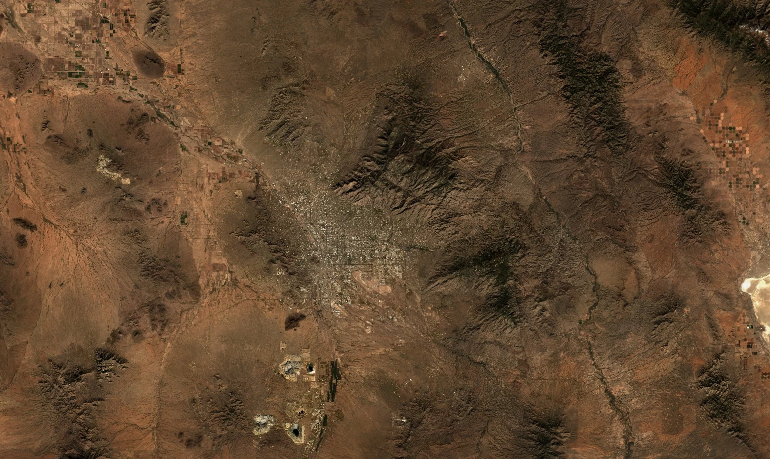
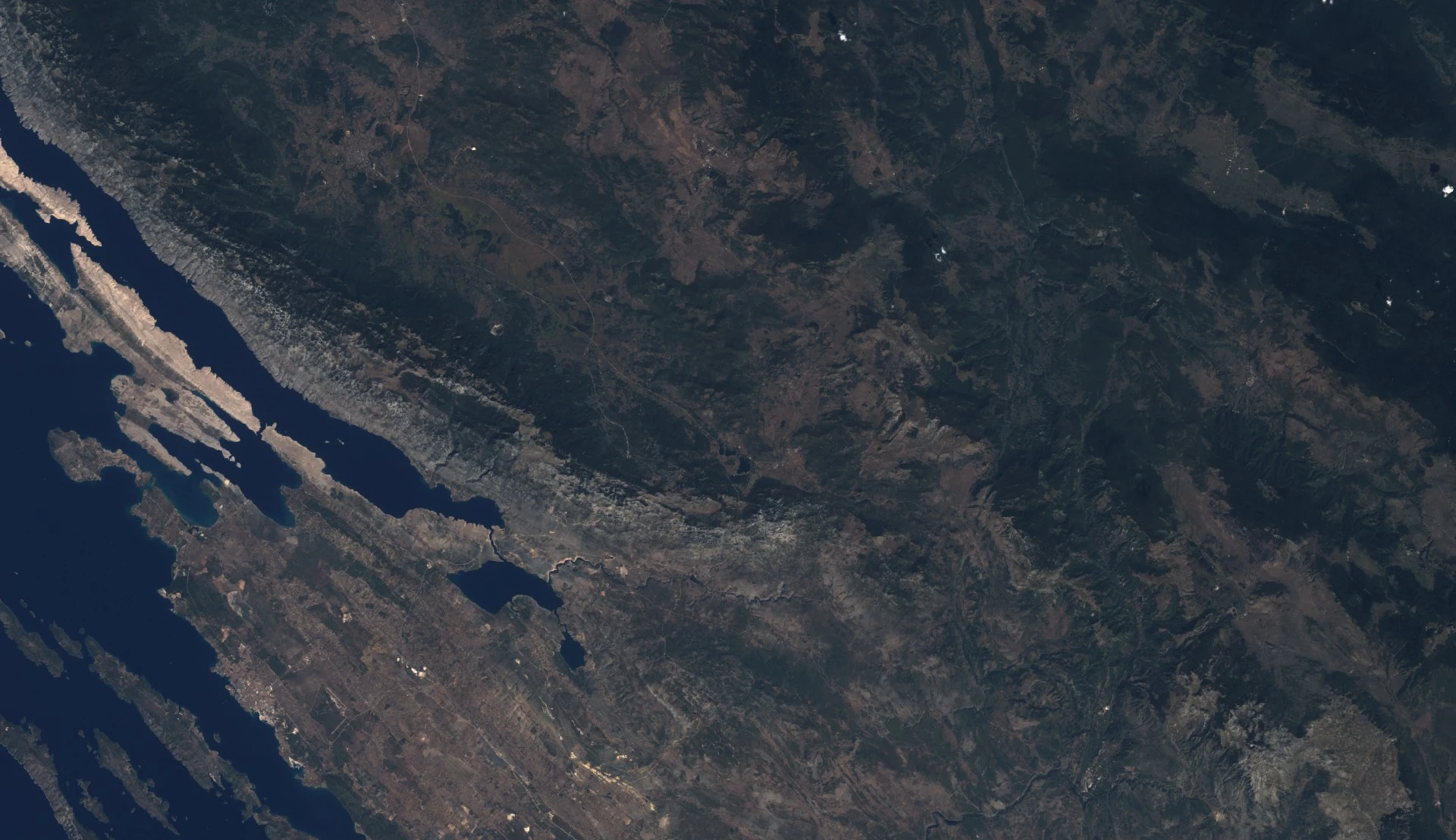
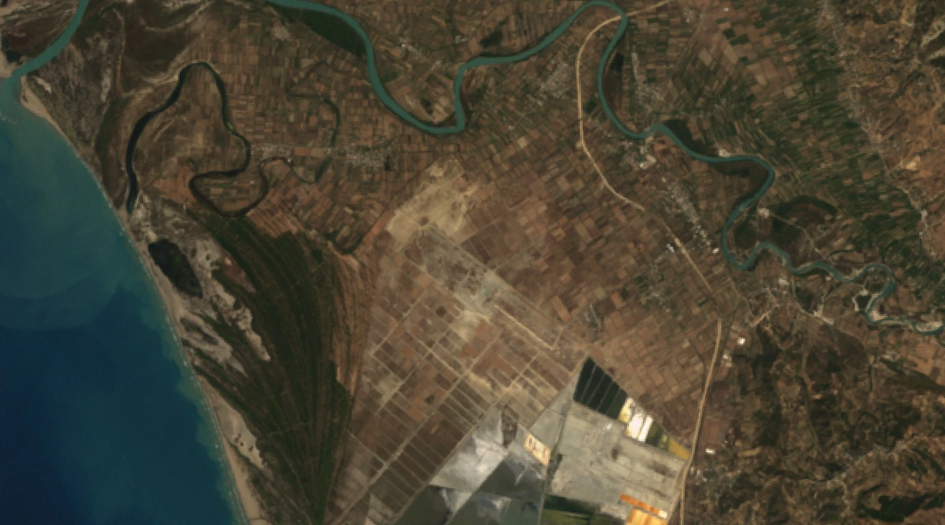
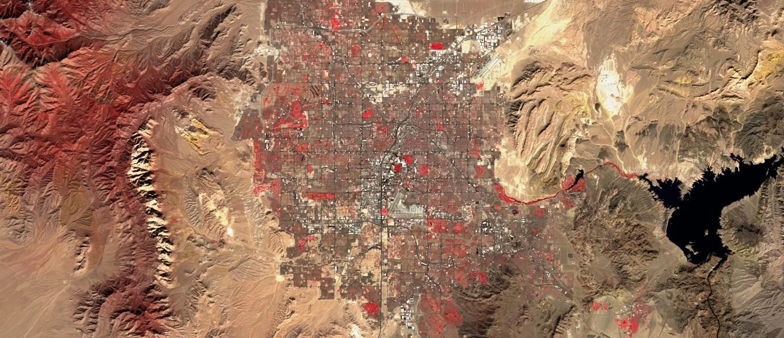

1 - data | | \[1]: Top of the Atmosphere Brightness Temperature. ### Scenes Object [`scenes` object](https://docs.planet.com/develop/evalscripts/functions.md#scenes) stores metadata. An example of metadata available in `scenes` object for HLS when mosaicking is `ORBIT`: | Property name | Value | | ----------------------- | -------------------------------------------------------------------------------------------- | | dateFrom | `'2018-12-25T00:00:00Z'` | | dateTo | `'2018-12-25T23:59:59Z'` | | tiles\[i].hlsProductId | `'HLSS30.020/HLS.S30.T58WEV.2020273T003609.v2.0`' | | tiles\[i].date | `'2018-12-25T09:45:29.121783Z'` | | tiles\[i].shId | `3097841` | | tiles\[i].cloudCoverage | `98.35` | | tiles\[i].dataPath | `'https://lp-prod-protected.s3.amazonaws.com/HLSS30.020/HLS.S30.T58WEV.2020273T003609.v2.0'` | Properties of a `scenes` object can differ depending on the selected mosaicking and in which evalscript function the object is accessed. [Working with metadata in evalscript](https://docs.planet.com/develop/evalscripts.md#working-with-metadata-in-evalscripts) user guide explains all details and provide examples. ## Catalog API Capabilities To access HLS product metadata you need to send search request to our [Catalog API](https://docs.planet.com/develop/apis/catalog/reference.md). The requested metadata will be returned as JSON formatted response to your request. ### Collection identifier: `hls` ### Filter extension * `eo:cloud_cover` cloud cover percentage * `constellation` ([possible values](#constellation)) ### Distinct extension * `date` --- Copy for LLM[View as Markdown](https://docs.planet.com/data/public-data/usgs-nasa/harmonized-landsat-sentinel/examples/) # Harmonized Landsat Sentinel Examples The following examples are CURL requests and can be run from the command line or terminal. In addition, you can copy and paste these examples into [Request Builder](https://insights.planet.com/analyze/requests-builder/). You can translate the requests into other programming languages in the Request Builder app. To request data using any of the request below, you will need to replace the string `` with your access token. Your access token will look something like this: ``` ayJhbGciOiJSUzI1NiJ9.ayJzdWIiOiI0MmYwODZjCy1kMzI3LTRlOTMtYWMxNS00ODAwOGFiZjI0YjIiLCJhdWQiOiJlY2I1MGM1Zi1i MWM1LTQ3ZTgtYWE4NC0zZTU4NzJlM2I2MTEiLCJqdGkiOiI5MzYxMWE4ODEyNTM4Y2M0MmU0NDJjYjUyMTY0YmJlNyIsImV4cCI6MTU1N TQyMzk3MiwibmFtZSI6ImFuamEudnJlY2tvQHNpbmVyZ2lzZS5jb20iLCJlbWFpbCI6ImFuamEudnJlY2tvQHNpbmVyZ2lzZS5jb20iLC JzaWQiOiIzZjVjZDVkNS04MjRiLTQ3ZjYtODgwNy0wNDMyNWY4ODQxZmQifQ.U7FPOy_2jlEOFxXSjyN5KEdBROna3-Dyec0feShIbUOY 1p9lEXdNaMmR5euiINi2RXDayX9Kr47CuSTsvq1zHFvZs1YgkFr1iH6kDuX-t_-wfWpqu5oPjoPVKZ4Rj0Ms_dxAUTQFTXR0rlbLuO-KS gnaeLVb5iiv_qY3Ctq2XKdIRcFRQLFziFcP4yZJl-NZMlwzsiiwjakcpYpI5jSYAdU2hpZLHRzceseeZt5YfZOe5Px1kZXro9Nd0L2GPC -qzOXw_V1saMGFa2ov8qV6Dvk92iv2SDDdGhOdII_JOf8XkK4E3g2z0EEFdWhG9F4Iky4ukNsqBPgE8LRb31s0hg ``` and can be obtained as described in the [Authentication chapter](https://docs.planet.com/develop/authentication.md). ## True Color ``` curl -X POST \ https://services-uswest2.sentinel-hub.com/process/v1 \ -H 'Authorization: Bearer ' \ -F 'request={ "input": { "bounds": { "properties": { "crs": "http://www.opengis.net/def/crs/OGC/1.3/CRS84" }, "bbox": [ 12.401213, 41.855754, 12.609214, 41.996243 ] }, "data": [{ "type": "hls", "dataFilter": { "timeRange": { "from": "2020-07-01T00:00:00Z", "to": "2020-07-31T00:00:00Z" } } }] }, "output": { "width": 512, "height": 512 } } ' \ -F 'evalscript=//VERSION=3 function setup() { return { input: ["Blue", "Green", "Red"], output: { bands: 3, sampleType: "AUTO" // default value - scales the output values from [0,1] to [0,255]. } } } function evaluatePixel(sample) { return [2.5 * sample.Red, 2.5 * sample.Green, 2.5 * sample.Blue] } ' ``` ## True Color, full 30 meter resolution (EPSG 32633) ``` curl -X POST \ https://services-uswest2.sentinel-hub.com/process/v1 \ -H 'Authorization: Bearer ' \ -F 'request={ "input": { "bounds": { "properties": { "crs": "http://www.opengis.net/def/crs/EPSG/0/32633" }, "bbox": [ 284281.024812, 4637026.521832, 301547.842435, 4652124.141629 ] }, "data": [{ "type": "hls", "dataFilter": { "timeRange": { "from": "2020-07-01T00:00:00Z", "to": "2020-07-31T00:00:00Z" } } }] }, "output": { "resx": 30, "resy": 30 } } ' \ -F 'evalscript=//VERSION=3 function setup() { return { input: ["Red", "Green", "Blue", "dataMask"], output: { bands: 4 } } } function evaluatePixel(sample) { return [2.5 * sample.Red, 2.5 * sample.Green, 2.5 * sample.Blue, sample.dataMask] } ' ``` ## NDVI as jpeg image with bounds given as polygon ``` curl -X POST \ https://services-uswest2.sentinel-hub.com/process/v1 \ -H 'Authorization: Bearer ' \ -F 'request={ "input": { "bounds": { "properties": { "crs": "http://www.opengis.net/def/crs/OGC/1.3/CRS84" }, "geometry": { "type": "Polygon", "coordinates": [ [ [ 12.480661, 41.965872 ], [ 12.523909, 41.96817 ], [ 12.553084, 41.931401 ], [ 12.525968, 41.906365 ], [ 12.491645, 41.894355 ], [ 12.449084, 41.896911 ], [ 12.433295, 41.926292 ], [ 12.442219, 41.950043 ], [ 12.480661, 41.965872 ] ] ] } }, "data": [{ "type": "hls", "dataFilter": { "timeRange": { "from": "2020-07-01T00:00:00Z", "to": "2020-07-31T00:00:00Z" } } }] }, "output": { "width": 512, "height": 512, "responses": [{ "identifier": "default", "format": { "type": "image/jpeg" } }] } } ' \ -F 'evalscript=//VERSION=3 function setup() { return { input: ["NIR_Narrow", "Red", "dataMask"], output: { bands: 4 } } } function evaluatePixel(sample) { var ndvi = (sample.NIR_Narrow - sample.Red) / (sample.NIR_Narrow + sample.Red) if (ndvi<-0.5) return [0.05,0.05,0.05,sample.dataMask] else if (ndvi<-0.2) return [0.75,0.75,0.75,sample.dataMask] else if (ndvi<-0.1) return [0.86,0.86,0.86,sample.dataMask] else if (ndvi<0) return [0.92,0.92,0.92,sample.dataMask] else if (ndvi<0.025) return [1,0.98,0.8,sample.dataMask] else if (ndvi<0.05) return [0.93,0.91,0.71,sample.dataMask] else if (ndvi<0.075) return [0.87,0.85,0.61,sample.dataMask] else if (ndvi<0.1) return [0.8,0.78,0.51,sample.dataMask] else if (ndvi<0.125) return [0.74,0.72,0.42,sample.dataMask] else if (ndvi<0.15) return [0.69,0.76,0.38,sample.dataMask] else if (ndvi<0.175) return [0.64,0.8,0.35,sample.dataMask] else if (ndvi<0.2) return [0.57,0.75,0.32,sample.dataMask] else if (ndvi<0.25) return [0.5,0.7,0.28,sample.dataMask] else if (ndvi<0.3) return [0.44,0.64,0.25,sample.dataMask] else if (ndvi<0.35) return [0.38,0.59,0.21,sample.dataMask] else if (ndvi<0.4) return [0.31,0.54,0.18,sample.dataMask] else if (ndvi<0.45) return [0.25,0.49,0.14,sample.dataMask] else if (ndvi<0.5) return [0.19,0.43,0.11,sample.dataMask] else if (ndvi<0.55) return [0.13,0.38,0.07,sample.dataMask] else if (ndvi<0.6) return [0.06,0.33,0.04,sample.dataMask] else return [0,0.27,0,sample.dataMask] }' ``` ## Exact NDVI values using a floating point GeoTIFF ``` curl -X POST \ https://services-uswest2.sentinel-hub.com/process/v1 \ -H 'Authorization: Bearer ' \ -F 'request={ "input": { "bounds": { "properties": { "crs": "http://www.opengis.net/def/crs/OGC/1.3/CRS84" }, "geometry": { "type": "Polygon", "coordinates": [ [ [ 12.480661, 41.965872 ], [ 12.523909, 41.96817 ], [ 12.553084, 41.931401 ], [ 12.525968, 41.906365 ], [ 12.491645, 41.894355 ], [ 12.449084, 41.896911 ], [ 12.433295, 41.926292 ], [ 12.442219, 41.950043 ], [ 12.480661, 41.965872 ] ] ] } }, "data": [{ "type": "hls", "dataFilter": { "timeRange": { "from": "2020-07-01T00:00:00Z", "to": "2020-07-31T00:00:00Z" } } }] }, "output": { "width": 512, "height": 512, "responses": [{ "identifier": "default", "format": { "type": "image/tiff" } }] } } ' \ -F 'evalscript=//VERSION=3 function setup() { return{ input: [{ bands: ["Red", "NIR_Narrow", "dataMask"] }], output: { id: "default", bands: 2, sampleType: SampleType.FLOAT32 } } } function evaluatePixel(sample) { let ndvi = (sample.NIR_Narrow - sample.Red) / (sample.NIR_Narrow + sample.Red) return [ ndvi, sample.dataMask ] }' ``` ## Landsat Thermal Band as jpeg image with bounds given as bounding box ``` curl -X POST \ https://services-uswest2.sentinel-hub.com/process/v1 \ -H 'Authorization: Bearer ' \ -F 'request={ "input": { "bounds": { "properties": { "crs": "http://www.opengis.net/def/crs/OGC/1.3/CRS84" }, "bbox": [ 12.401213, 41.855754, 12.609214, 41.996243 ] }, "data": [{ "type": "hls", "dataFilter": { "timeRange": { "from": "2020-07-01T00:00:00Z", "to": "2020-07-31T00:00:00Z" }, "constellation": "LANDSAT" } }] }, "output": { "width": 512, "height": 512, "responses": [{ "identifier": "default", "format": { "type": "image/png" } }] } } ' \ -F 'evalscript=//VERSION=3 let minVal = -50 let maxVal = 50 let viz = ColorGradientVisualizer.createBlueRed(minVal, maxVal) function setup() { return { input: [{ bands: [ "ThermalInfrared1", "dataMask" ] }], output: { bands: 4 } } } function evaluatePixel(samples) { let val = samples.ThermalInfrared1 val = viz.process(val) val.push(samples.dataMask) return val } ' ``` ## Landsat Thermal band Kelvin values using a FLOAT32 GeoTIFF ``` curl -X POST \ https://services-uswest2.sentinel-hub.com/process/v1 \ -H 'Authorization: Bearer ' \ -F 'request={ "input": { "bounds": { "properties": { "crs": "http://www.opengis.net/def/crs/OGC/1.3/CRS84" }, "bbox": [ 12.401213, 41.855754, 12.609214, 41.996243 ] }, "data": [{ "type": "hls", "dataFilter": { "timeRange": { "from": "2020-07-01T00:00:00Z", "to": "2020-07-31T00:00:00Z" }, "constellation": "LANDSAT" } }] }, "output": { "width": 512, "height": 512, "responses": [{ "identifier": "default", "format": { "type": "image/tiff" } }] } } ' \ -F 'evalscript=//VERSION=3 function setup() { return { input: [{ bands: [ "ThermalInfrared1", "dataMask" ] }], output: { bands: 2, sampleType: "FLOAT32" } } } function evaluatePixel(samples) { return [samples.ThermalInfrared1, samples.dataMask] } ' ``` ## Sentinel Red Edge Composite ``` curl -X POST \ https://services-uswest2.sentinel-hub.com/process/v1 \ -H 'Authorization: Bearer ' \ -F 'request={ "input": { "bounds": { "properties": { "crs": "http://www.opengis.net/def/crs/OGC/1.3/CRS84" }, "bbox": [ 12.401213, 41.855754, 12.609214, 41.996243 ] }, "data": [{ "type": "hls", "dataFilter": { "timeRange": { "from": "2022-07-01T00:00:00Z", "to": "2022-07-31T00:00:00Z" }, "constellation": "SENTINEL" } }] }, "output": { "width": 512, "height": 512, "responses": [{ "identifier": "default", "format": { "type": "image/png" } }] } } ' \ -F 'evalscript= //VERSION=3 function setup() { return { input: [{ bands: [ "RedEdge3", "RedEdge2", "RedEdge1", "dataMask" ] }], output: { bands: 4 } } } function evaluatePixel(samples) { return [3*samples.RedEdge3, 3*samples.RedEdge2, 3*samples.RedEdge1, samples.dataMask] } ' ``` ## Sentinel True color and metadata (multi-part response GeoTIFF and json) ``` curl -X POST \ https://services-uswest2.sentinel-hub.com/process/v1 \ -H 'Authorization: Bearer ' \ -H 'accept: application/tar' \ -F 'request={ "input": { "bounds": { "bbox": [ 12.401213, 41.855754, 12.609214, 41.996243 ] }, "data": [{ "type": "hls", "dataFilter": { "timeRange": { "from": "2022-07-01T00:00:00Z", "to": "2022-07-31T00:00:00Z" }, "constellation": "SENTINEL" } }] }, "output": { "width": 512, "height": 512, "responses": [{ "identifier": "default", "format": { "type": "image/tiff" } }, { "identifier": "userdata", "format": { "type": "application/json" } } ] } } ' \ -F 'evalscript=//VERSION=3 function setup() { return { input: ["Blue", "Green", "Red", "dataMask"], mosaicking: Mosaicking.ORBIT, output: { id: "default", bands: 4 } } } function updateOutputMetadata(scenes, inputMetadata, outputMetadata) { outputMetadata.userData = { "scenes": scenes.orbits } } function evaluatePixel(samples) { return [2.5 * samples[0].Red, 2.5 * samples[0].Green, 2.5 * samples[0].Blue, samples.dataMask] } ' ``` ## True color multi-part response (different formats and SampleType) ``` curl -X POST \ https://services-uswest2.sentinel-hub.com/process/v1 \ -H 'Authorization: Bearer ' \ -H 'Accept: application/tar' \ -F 'request={ "input": { "bounds": { "properties": { "crs": "http://www.opengis.net/def/crs/OGC/1.3/CRS84" }, "bbox": [ 12.401213, 41.855754, 12.609214, 41.996243 ] }, "data": [{ "type": "hls", "dataFilter": { "timeRange": { "from": "2020-07-01T00:00:00Z", "to": "2020-07-31T00:00:00Z" } } }] }, "output": { "width": 512, "height": 512, "responses": [{ "identifier": "true_color", "format": { "type": "image/jpeg" } }, { "identifier": "true_color_8bit", "format": { "type": "image/png" } }, { "identifier": "true_color_16bit", "format": { "type": "image/tiff" } }, { "identifier": "true_color_32float", "format": { "type": "image/tiff" } } ] } } ' \ -F 'evalscript=//VERSION=3 function setup() { return { input: [{ bands: ["Red", "Green", "Blue"], units: "REFLECTANCE" // default units }], output: [{ id: "true_color", bands: 3, sampleType: "AUTO" // default - scales the output values from input values [0,1] to [0,255]. }, { id: "true_color_8bit", bands: 3, sampleType: "UINT8" }, { id: "true_color_16bit", bands: 3, sampleType: "UINT16" //floating point values are automatically rounded to the nearest integer by the service. }, { id: "true_color_32float", bands: 3, sampleType: "FLOAT32" } ] } } function evaluatePixel(sample) { return { // output band values are scaled from [0,1] to [0,255]. Multiply by 2.5 to increase brightness true_color: [2.5 * sample.Red, 2.5 * sample.Green, 2.5 * sample.Blue], // Multiply input reflectance values by 255 to stretch them to [0, 255] unsigned 8 bit range. true_color_8bit: [sample.Red * 255, sample.Green * 255, sample.Blue * 255], // Multiply input reflectance values by 65535 to stretch them to [0, 65535] unsigned 16 bit range. true_color_16bit: [sample.Red * 65535, sample.Green * 65535, sample.Blue * 65535], // Reflectance values true_color_32float: [sample.Red, sample.Green, sample.Blue], } } ' ``` ## HLS bands from both constellations as GeoTIFF ``` curl -X POST https://services-uswest2.sentinel-hub.com/process/v1 \ -H 'Authorization: Bearer ' \ -F 'request={ "input": { "bounds": { "bbox": [ 12.401213, 41.855754, 12.609214, 41.996243 ] }, "data": [ { "dataFilter": { "timeRange": { "from": "2020-07-01T00:00:00Z", "to": "2020-07-31T23:59:59Z" } }, "type": "hls" } ] }, "output": { "width": 512, "height": 464.292, "responses": [ { "identifier": "default", "format": { "type": "image/tiff" } } ] } }' \ -F 'evalscript=//VERSION=3 function setup() { return { input: [{ bands: ["CoastalAerosol", "Blue", "Green", "Red", "NIR_Narrow", "SWIR1", "SWIR2", "Cirrus", "QA"] }], output: { id: "default", bands: 9, sampleType: SampleType.UINT16 //floating point values are automatically rounded to the nearest integer by the service. } } } function evaluatePixel(sample) { // For optical bands, return reflectance multiplied by 10000 as integers to save processing units. To obtain reflectance values, simply divide the resulting pixel values by 10000. return [10000 * sample.CoastalAerosol, 10000 * sample.Blue, 10000 * sample.Green, 10000 * sample.Red, 10000 * sample.NIR_Narrow, 10000 * sample.SWIR1, 10000 * sample.SWIR2, 1000* sample.Cirrus, sample.QA] }' ``` ## Only HLS Sentinel-2 bands as GeoTIFF ``` curl -X POST https://services-uswest2.sentinel-hub.com/process/v1 \ -H 'Authorization: Bearer ' \ -F 'request={ "input": { "bounds": { "bbox": [ 12.401213, 41.855754, 12.609214, 41.996243 ] }, "data": [ { "dataFilter": { "timeRange": { "from": "2020-07-01T00:00:00Z", "to": "2020-07-31T23:59:59Z" }, "constellation": "SENTINEL" }, "type": "hls" } ] }, "output": { "width": 512, "height": 464.292, "responses": [ { "identifier": "default", "format": { "type": "image/tiff" } } ] } }' \ -F 'evalscript=//VERSION=3 function setup() { return { input: [{ bands: ["CoastalAerosol", "Blue", "Green", "Red", "RedEdge1", "RedEdge2", "RedEdge3", "NIR_Broad", "NIR_Narrow", "SWIR1", "SWIR2", "Cirrus", "QA"] }], output: { id: "default", bands: 13, sampleType: SampleType.UINT16 //floating point values are automatically rounded to the nearest integer by the service. } } } function evaluatePixel(sample) { // For optical bands, return reflectance multiplied by 10000 as integers to save processing units. To obtain reflectance values, simply divide the resulting pixel values by 10000. return [10000 * sample.CoastalAerosol, 10000 * sample.Blue, 10000 * sample.Green, 10000 * sample.Red, 10000 * sample.RedEdge1, 10000 * sample.RedEdge2, 10000 * sample.RedEdge3, 1000* sample.NIR_Broad, 10000 * sample.NIR_Narrow, 10000 * sample.SWIR1, 10000 * sample.SWIR2, 1000* sample.Cirrus, sample.QA] }' ``` ## Only HLS Landsat8/9 bands as GeoTIFF ``` curl -X POST https://services-uswest2.sentinel-hub.com/process/v1 \ -H 'Authorization: Bearer ' \ -F 'request={ "input": { "bounds": { "bbox": [ 12.401213, 41.855754, 12.609214, 41.996243 ] }, "data": [ { "dataFilter": { "timeRange": { "from": "2020-07-01T00:00:00Z", "to": "2020-07-31T23:59:59Z" }, "constellation": "LANDSAT" }, "type": "hls" } ] }, "output": { "width": 512, "height": 464.292, "responses": [ { "identifier": "default", "format": { "type": "image/tiff" } } ] } }' \ -F 'evalscript=//VERSION=3 function setup() { return { input: [{ bands: ["CoastalAerosol", "Blue", "Green", "Red", "NIR_Narrow", "SWIR1", "SWIR2", "Cirrus", "ThermalInfrared1", "ThermalInfrared2", "QA"] }], output: { id: "default", bands: 11, sampleType: SampleType.UINT16 //floating point values are automatically rounded to the nearest integer by the service. } } } function evaluatePixel(sample) { // For optical bands, return reflectance multiplied by 10000 as integers to save processing units. To obtain reflectance values, simply divide the resulting pixel values by 10000. return [10000 * sample.CoastalAerosol, 10000 * sample.Blue, 10000 * sample.Green, 10000 * sample.Red, 10000 * sample.NIR_Narrow, 10000 * sample.SWIR1, 10000 * sample.SWIR2, 1000* sample.Cirrus, sample.ThermalInfrared1, sample.ThermalInfrared2, sample.QA] }' ``` --- Copy for LLM[View as Markdown](https://docs.planet.com/data/public-data/usgs-nasa/landsat-4-5-tm/) # Landsat 4-5 TM L1 & L2 ![Header Thumbnail](/data/public-data/landsat-4-5-tm/thumbnail.webp) The Landsat Thematic Mapper (TM) sensor was carried onboard Landsats 4 and 5. It provides 6 spectral bands and 1 thermal infrared band. Landsat 4–5 TM Collection 2 includes both Level 1 and Level 2 products, supporting long-term global Earth observation from the early 1980s through 2012. Landsat 4–5 TM Level 1 products provide radiometrically calibrated and orthorectified Top-of-Atmosphere (TOA) reflectance and brightness temperature data. Landsat 4–5 TM Level 2 products provide atmospherically corrected surface reflectance and surface temperature science products derived from Collection 2 Level 1 inputs. ## Basic Facts | Property | Landsat 4–5 TM Level 1 | Landsat 4–5 TM Level 2 | | ------------------------ | -------------------------------------------------------------------------- | -------------------------------------------------------------------------- | | **Data type** | TOA Reflectance and Brightness Temperature | Surface Reflectance and Surface Temperature | | **Spatial resolution** | 30 m (thermal band resampled from 120 m) | 30 m (thermal band resampled from 120 m) | | **Sensor** | Thematic Mapper (TM) with 6 spectral bands and 1 thermal infrared band | Thematic Mapper (TM) with 6 spectral bands and 1 thermal infrared band | | **Revisit time** | 16 days | 16 days | | **Spatial coverage** | Whole globe | Whole globe | | **Data availability** | Landsat 4: Aug 1982 – Dec 1993

Landsat 5: Mar 1984 – May 2012 | Landsat 4: Aug 1982 – Dec 1993
Landsat 5: Mar 1984 – May 2012 | | **Common usage/purpose** | Vegetation monitoring, land use, land cover maps and monitoring of changes | Vegetation monitoring, land use, land cover maps and monitoring of changes | ## Accessing Data To access data you need to send a POST request to our `process` API. The requested data will be returned as the response to your request. Each POST request can be tailored to get you exactly the data you require. To do this requires setting various parameters which depend on the collection you are querying. For an overview of all API parameters see the [API Reference](https://docs.planet.com/develop/apis/processing/reference.md). ### Endpoint Locations | Service | Notes | | ------------------------------------- | ------------------------------------------ | | services-uswest2.sentinel-hub.com/api | Global coverage from July 1982 to May 2012 | ### Data type identifiers Use the following values for `input.data.type`: | Dataset | Identifier | | ---------------------- | --------------- | | Landsat 4–5 TM Level 1 | `landsat-tm-l1` | | Landsat 4–5 TM Level 2 | `landsat-tm-l2` | ## Filtering Options This chapter explains the `input.data.dataFilter` object of the `process` API. ### `mosaickingOrder` Sets the order of overlapping tiles from which the output result is mosaicked. Note that tiles will in most cases come from the same orbit/acquisition. The tiling is done by USGS for easier distribution. | Value | Description | Notes | | --------------- | ------------------------------------------------------------------------- | --------------------------------------------------------------------- | | **mostRecent** | (default) The pixel will be selected from the most recently acquired tile | | | **leastRecent** | similar to **mostRecent** but in reverse order | | | **leastCC** | The pixel is selected from the tile with the lowest cloud coverage | Estimated per tile (\~31,000 sq. km); local cloud coverage may differ | ### `maxCloudCoverage` Sets the upper limit for cloud coverage in percent based on the precomputed cloud coverage estimate for each tile as present in the tile metadata. ### `tiers` | Value | Description | | -------------- | ------------------------------------------------------- | | **TIER\_1** | selects Tier 1 products | | **ALL\_TIERS** | selected by default. selects Tier 1 and Tier 2 products | ## Processing Options This chapter explains the `input.data.processing` object of the `process` API. | Parameter | Description | | ------------ | ----------------------------------------------------------------------------------------------------------- | | upsampling | [Same as Sentinel-2.](https://docs.planet.com/data/public-data/copernicus/sentinel-2.md#processing-options) | | downsampling | [Same as Sentinel-2.](https://docs.planet.com/data/public-data/copernicus/sentinel-2.md#processing-options) | ## Available Bands and Data ### Landsat 4–5 TM Level 1 Bands | Name | Description | Resolution | | ---------- | ---------------------------------------------------- | ---------- | | B01 | Blue (450–520 nm) | 30 m | | B02 | Green (520–600 nm) | 30 m | | B03 | Red (630–690 nm) | 30 m | | B04 | Near Infrared (760–900 nm) | 30 m | | B05 | SWIR 1 (1550–1750 nm) | 30 m | | B06 | Thermal Infrared (10400–12500 nm) | 30 m \[1] | | B07 | SWIR 2 (2080–2350 nm) | 30 m | | BQA | Quality Assessment band | 30 m | | QA\_RADSAT | Radiometric Saturation and Terrain Occlusion QA Band | 30 m | | VAA | View Azimuth Angle | 30 m | | VZA | View Zenith Angle | 30 m | | SAA | Sun Azimuth Angle | 30 m | | SZA | Sun Zenith Angle | 30 m | | dataMask | Data / no-data mask | N/A | \[1]: Thermal band is acquired at 120 m and resampled to 30 m. ### Landsat 4–5 TM Level 2 Bands Includes all Level 1 bands plus surface reflectance and surface temperature–related products: | Name | Description | Resolution | | ------------------ | ------------------------------- | ---------- | | B01–B05, B07 | Surface reflectance bands | 30 m | | B06 | Surface temperature | 30 m | | ST\_QA | Surface Temperature Uncertainty | 30 m | | ST\_TRAD | Thermal surface radiance | 30 m | | ST\_URAD | Upwelled radiance | 30 m | | ST\_DRAD | Downwelled radiance | 30 m | | ST\_ATRAN | Atmospheric transmittance | 30 m | | ST\_EMIS | Emissivity | 30 m | | ST\_EMSD | Emissivity standard deviation | 30 m | | ST\_CDIST | Pixel distance to cloud | 30 m | | SR\_ATMOS\_OPACITY | Atmospheric opacity | 30 m | | SR\_CLOUD\_QA | Cloud Quality Assessment | 30 m | | dataMask | Data / no-data mask | N/A | ## Units Both Level 1 and Level 2 units are preserved exactly as defined in the original pages. * **Level 1**: TOA Reflectance and Brightness Temperature * **Level 2**: Surface Reflectance and Surface Temperature (See original unit tables for full band-level details.) ## Scenes Object The [`scenes` object](https://docs.planet.com/develop/evalscripts/functions.md#scenes) stores metadata returned with Processing API responses. Properties may differ depending on mosaicking and product level. ## Catalog API Capabilities To access Landsat 4–5 TM metadata, send a search request to our [Catalog API](https://docs.planet.com/develop/apis/catalog/reference.md). ### Collection identifiers * `landsat-tm-l1` * `landsat-tm-l2` ### Filter extension * `eo:cloud_cover` * `landsat:scene_id` * `landsat:collection_category` ### Distinct extension * `date` --- Copy for LLM[View as Markdown](https://docs.planet.com/data/public-data/usgs-nasa/landsat-4-5-tm/examples/) # Landsat 4-5 TM L1 & L2 Examples The following examples are CURL requests and can be run from the command line or terminal. In addition, you can copy and paste these examples into [Request Builder](https://insights.planet.com/analyze/requests-builder/). You can translate the requests into other programming languages in the Request Builder app. To request data using any of the request below, you will need to replace the string `` with your access token. Your access token will look something like this: ``` ayJhbGciOiJSUzI1NiJ9.ayJzdWIiOiI0MmYwODZjCy1kMzI3LTRlOTMtYWMxNS00ODAwOGFiZjI0YjIiLCJhdWQiOiJlY2I1MGM1Zi1i MWM1LTQ3ZTgtYWE4NC0zZTU4NzJlM2I2MTEiLCJqdGkiOiI5MzYxMWE4ODEyNTM4Y2M0MmU0NDJjYjUyMTY0YmJlNyIsImV4cCI6MTU1N TQyMzk3MiwibmFtZSI6ImFuamEudnJlY2tvQHNpbmVyZ2lzZS5jb20iLCJlbWFpbCI6ImFuamEudnJlY2tvQHNpbmVyZ2lzZS5jb20iLC JzaWQiOiIzZjVjZDVkNS04MjRiLTQ3ZjYtODgwNy0wNDMyNWY4ODQxZmQifQ.U7FPOy_2jlEOFxXSjyN5KEdBROna3-Dyec0feShIbUOY 1p9lEXdNaMmR5euiINi2RXDayX9Kr47CuSTsvq1zHFvZs1YgkFr1iH6kDuX-t_-wfWpqu5oPjoPVKZ4Rj0Ms_dxAUTQFTXR0rlbLuO-KS gnaeLVb5iiv_qY3Ctq2XKdIRcFRQLFziFcP4yZJl-NZMlwzsiiwjakcpYpI5jSYAdU2hpZLHRzceseeZt5YfZOe5Px1kZXro9Nd0L2GPC -qzOXw_V1saMGFa2ov8qV6Dvk92iv2SDDdGhOdII_JOf8XkK4E3g2z0EEFdWhG9F4Iky4ukNsqBPgE8LRb31s0hg ``` and can be obtained as described in the [Authentication chapter](https://docs.planet.com/develop/authentication.md). ## True Color * L2 ``` curl -X POST \ https://services-uswest2.sentinel-hub.com/process/v1 \ -H 'Authorization: Bearer ' \ -F 'request={ "input": { "bounds": { "properties": { "crs": "http://www.opengis.net/def/crs/OGC/1.3/CRS84" }, "bbox": [ 12.401213, 41.855754, 12.609214, 41.996243 ] }, "data": [{ "type": "landsat-tm-l2", "dataFilter": { "timeRange": { "from": "2010-07-01T00:00:00Z", "to": "2010-07-31T00:00:00Z" } } }] }, "output": { "width": 512, "height": 512 } } ' \ -F 'evalscript=//VERSION=3 function setup() { return { input: ["B01", "B02", "B03"], output: { bands: 3, sampleType: "AUTO" // default value - scales the output values from [0,1] to [0,255]. } } } function evaluatePixel(sample) { return [2.5 * sample.B03, 2.5 * sample.B02, 2.5 * sample.B01] } ' ``` ## True Color, resolution (EPSG 32633) * L2 ``` curl -X POST \ https://services-uswest2.sentinel-hub.com/process/v1 \ -H 'Authorization: Bearer ' \ -F 'request={ "input": { "bounds": { "properties": { "crs": "http://www.opengis.net/def/crs/EPSG/0/32633" }, "bbox": [ 408553.58, 5078145.48, 466081.02, 5126576.61 ] }, "data": [{ "type": "landsat-tm-l2", "dataFilter": { "timeRange": { "from": "2010-07-01T00:00:00Z", "to": "2010-07-31T00:00:00Z" } } }] }, "output": { "resx": 100, "resy": 100 } } ' \ -F 'evalscript=//VERSION=3 function setup() { return { input: ["B01", "B02", "B03"], output: { bands: 3 } } } function evaluatePixel(sample) { return [2.5 * sample.B03, 2.5 * sample.B02, 2.5 * sample.B01] } ' ``` ## True Color, multi-band GeoTIFF * L2 ``` curl -X POST \ https://services-uswest2.sentinel-hub.com/process/v1 \ -H 'Authorization: Bearer ' \ -F 'request={ "input": { "bounds": { "properties": { "crs": "http://www.opengis.net/def/crs/OGC/1.3/CRS84" }, "bbox": [ 12.401213, 41.855754, 12.609214, 41.996243 ] }, "data": [{ "type": "landsat-tm-l2", "dataFilter": { "timeRange": { "from": "2010-07-01T00:00:00Z", "to": "2010-07-31T00:00:00Z" } } }] }, "output": { "width": 512, "height": 512 } } ' \ -F 'evalscript=//VERSION=3 function setup() { return { input: ["B01", "B02", "B03"], output: { bands: 3 } } } function evaluatePixel(sample) { return [2.5 * sample.B03, 2.5 * sample.B02, 2.5 * sample.B01] } ' ``` ## True Color, mosaicking with leastRecent * L2 ``` curl -X POST \ https://services-uswest2.sentinel-hub.com/process/v1 \ -H 'Authorization: Bearer ' \ -F 'request={ "input": { "bounds": { "properties": { "crs": "http://www.opengis.net/def/crs/OGC/1.3/CRS84" }, "bbox": [ 12.401213, 41.855754, 12.609214, 41.996243 ] }, "data": [{ "type": "landsat-tm-l2", "dataFilter": { "timeRange": { "from": "2010-07-01T00:00:00Z", "to": "2010-07-31T00:00:00Z" }, "mosaickingOrder": "leastRecent" } }] }, "output": { "width": 512, "height": 512, "responses": [{ "identifier": "default", "format": { "type": "image/png" } }] } } ' \ -F 'evalscript=//VERSION=3 function setup() { return { input: ["B01", "B02", "B03"], output: { bands: 3 } } } function evaluatePixel(sample) { return [2.5 * sample.B01, 2.5 * sample.B02, 2.5 * sample.B03] } ' ``` ## True Color and metadata (multi-part response GeoTIFF and json) * L2 ``` curl -X POST \ https://services-uswest2.sentinel-hub.com/process/v1 \ -H 'Authorization: Bearer ' \ -H 'accept: application/tar' \ -F 'request={ "input": { "bounds": { "bbox": [ 12.401213, 41.855754, 12.609214, 41.996243 ] }, "data": [{ "type": "landsat-tm-l2", "dataFilter": { "timeRange": { "from": "2010-07-01T00:00:00Z", "to": "2010-07-31T00:00:00Z" } } }] }, "output": { "width": 512, "height": 512, "responses": [{ "identifier": "default", "format": { "type": "image/tiff" } }, { "identifier": "userdata", "format": { "type": "application/json" } } ] } } ' \ -F 'evalscript=//VERSION=3 function setup() { return { input: ["B01", "B02", "B03"], mosaicking: Mosaicking.ORBIT, output: { id: "default", bands: 3 } } } function updateOutputMetadata(scenes, inputMetadata, outputMetadata) { outputMetadata.userData = { "scenes": scenes.orbits } } function evaluatePixel(samples) { return [2.5 * samples[0].B03, 2.5 * samples[0].B02, 2.5 * samples[0].B01] } ' ``` ## True Color multi-part response (different formats and SampleType) * L2 ``` curl -X POST \ https://services-uswest2.sentinel-hub.com/process/v1 \ -H 'Authorization: Bearer ' \ -H 'Accept: application/tar' \ -F 'request={ "input": { "bounds": { "properties": { "crs": "http://www.opengis.net/def/crs/OGC/1.3/CRS84" }, "bbox": [ 12.401213, 41.855754, 12.609214, 41.996243 ] }, "data": [{ "type": "landsat-tm-l2", "dataFilter": { "timeRange": { "from": "2010-07-01T00:00:00Z", "to": "2010-07-31T00:00:00Z" } } }] }, "output": { "width": 512, "height": 512, "responses": [{ "identifier": "true_color", "format": { "type": "image/jpeg" } }, { "identifier": "true_color_8bit", "format": { "type": "image/png" } }, { "identifier": "true_color_16bit", "format": { "type": "image/tiff" } }, { "identifier": "true_color_32float", "format": { "type": "image/tiff" } } ] } } ' \ -F 'evalscript=//VERSION=3 function setup() { return { input: [{ bands: ["B01", "B02", "B03"], units: "REFLECTANCE" // default units }], output: [{ id: "true_color", bands: 3, sampleType: "AUTO" // default - scales the output values from input values [0,1] to [0,255]. }, { id: "true_color_8bit", bands: 3, sampleType: "UINT8" }, { id: "true_color_16bit", bands: 3, sampleType: "UINT16" //floating point values are automatically rounded to the nearest integer by the service. }, { id: "true_color_32float", bands: 3, sampleType: "FLOAT32" } ] } } function evaluatePixel(sample) { return { // output band values are scaled from [0,1] to [0,255]. Multiply by 2.5 to increase brightness true_color: [2.5 * sample.B03, 2.5 * sample.B02, 2.5 * sample.B01], // Multiply input reflectance values by 255 to stretch them to [0, 255] unsigned 8 bit range. true_color_8bit: [sample.B03 * 255, sample.B02 * 255, sample.B01 * 255], // Multiply input reflectance values by 65535 to stretch them to [0, 65535] unsigned 16 bit range. true_color_16bit: [sample.B03 * 65535, sample.B02 * 65535, sample.B01 * 65535], // Reflectance values true_color_32float: [sample.B03, sample.B02, sample.B01], } } ' ``` ## NDVI as jpeg image with bounds given as polygon * L2 ``` curl -X POST \ https://services-uswest2.sentinel-hub.com/process/v1 \ -H 'Authorization: Bearer ' \ -F 'request={ "input": { "bounds": { "properties": { "crs": "http://www.opengis.net/def/crs/OGC/1.3/CRS84" }, "geometry": { "type": "Polygon", "coordinates": [ [ [ 12.480661, 41.965872 ], [ 12.523909, 41.96817 ], [ 12.553084, 41.931401 ], [ 12.525968, 41.906365 ], [ 12.491645, 41.894355 ], [ 12.449084, 41.896911 ], [ 12.433295, 41.926292 ], [ 12.442219, 41.950043 ], [ 12.480661, 41.965872 ] ] ] } }, "data": [{ "type": "landsat-tm-l2", "dataFilter": { "timeRange": { "from": "2010-07-01T00:00:00Z", "to": "2010-07-31T00:00:00Z" } } }] }, "output": { "width": 512, "height": 512, "responses": [{ "identifier": "default", "format": { "type": "image/jpeg", "quality": 80 } }] } } ' \ -F 'evalscript=//VERSION=3 function setup() { return { input: [{ bands:["B03", "B04"], }], output: { id: "default", bands: 3, } } } function evaluatePixel(sample) { let ndvi = (sample.B04 - sample.B03) / (sample.B04 + sample.B03) if (ndvi<-0.5) return [0.05,0.05,0.05] else if (ndvi<-0.2) return [0.75,0.75,0.75] else if (ndvi<-0.1) return [0.86,0.86,0.86] else if (ndvi<0) return [0.92,0.92,0.92] else if (ndvi<0.025) return [1,0.98,0.8] else if (ndvi<0.05) return [0.93,0.91,0.71] else if (ndvi<0.075) return [0.87,0.85,0.61] else if (ndvi<0.1) return [0.8,0.78,0.51] else if (ndvi<0.125) return [0.74,0.72,0.42] else if (ndvi<0.15) return [0.69,0.76,0.38] else if (ndvi<0.175) return [0.64,0.8,0.35] else if (ndvi<0.2) return [0.57,0.75,0.32] else if (ndvi<0.25) return [0.5,0.7,0.28] else if (ndvi<0.3) return [0.44,0.64,0.25] else if (ndvi<0.35) return [0.38,0.59,0.21] else if (ndvi<0.4) return [0.31,0.54,0.18] else if (ndvi<0.45) return [0.25,0.49,0.14] else if (ndvi<0.5) return [0.19,0.43,0.11] else if (ndvi<0.55) return [0.13,0.38,0.07] else if (ndvi<0.6) return [0.06,0.33,0.04] else return [0,0.27,0] }' ``` ## Exact NDVI values using a floating point GeoTIFF * L2 ``` curl -X POST \ https://services-uswest2.sentinel-hub.com/process/v1 \ -H 'Authorization: Bearer ' \ -F 'request={ "input": { "bounds": { "properties": { "crs": "http://www.opengis.net/def/crs/OGC/1.3/CRS84" }, "geometry": { "type": "Polygon", "coordinates": [ [ [ 12.480661, 41.965872 ], [ 12.523909, 41.96817 ], [ 12.553084, 41.931401 ], [ 12.525968, 41.906365 ], [ 12.491645, 41.894355 ], [ 12.449084, 41.896911 ], [ 12.433295, 41.926292 ], [ 12.442219, 41.950043 ], [ 12.480661, 41.965872 ] ] ] } }, "data": [{ "type": "landsat-tm-l2", "dataFilter": { "timeRange": { "from": "2010-07-01T00:00:00Z", "to": "2010-07-31T00:00:00Z" } } }] }, "output": { "width": 512, "height": 512, "responses": [{ "identifier": "default", "format": { "type": "image/tiff" } }] } } ' \ -F 'evalscript=//VERSION=3 function setup() { return{ input: [{ bands: ["B03", "B04"] }], output: { id: "default", bands: 1, sampleType: SampleType.FLOAT32 } } } function evaluatePixel(sample) { let ndvi = (sample.B04 - sample.B03) / (sample.B04 + sample.B03) return [ ndvi ] }' ``` ## NDVI image and value (multi-part response png and GeoTIFF) * L2 ``` curl -X POST \ https://services-uswest2.sentinel-hub.com/process/v1 \ -H 'Authorization: Bearer ' \ -H 'Accept: application/tar' \ -F 'request={ "input": { "bounds": { "properties": { "crs": "http://www.opengis.net/def/crs/OGC/1.3/CRS84" }, "geometry": { "type": "Polygon", "coordinates": [ [ [ 12.480661, 41.965872 ], [ 12.523909, 41.96817 ], [ 12.553084, 41.931401 ], [ 12.525968, 41.906365 ], [ 12.491645, 41.894355 ], [ 12.449084, 41.896911 ], [ 12.433295, 41.926292 ], [ 12.442219, 41.950043 ], [ 12.480661, 41.965872 ] ] ] } }, "data": [{ "type": "landsat-tm-l2", "dataFilter": { "timeRange": { "from": "2010-07-01T00:00:00Z", "to": "2010-07-31T00:00:00Z" } } }] }, "output": { "width": 512, "height": 512, "responses": [{ "identifier": "ndvi_image", "format": { "type": "image/png" } }, { "identifier": "default", "format": { "type": "image/tiff" } } ] } } ' \ -F 'evalscript=//VERSION=3 function setup() { return { input: [{ bands: ["B03", "B04"], }], output: [{ id: "default", bands: 1, sampleType: SampleType.FLOAT32 }, { id: "ndvi_image", bands: 3, sampleType: SampleType.AUTO } ] } } function evaluatePixel(sample) { let ndvi = (sample.B04 - sample.B03) / (sample.B04 + sample.B03) if (ndvi < -0.5) image = [0.05, 0.05, 0.05] else if (ndvi < -0.2) image = [0.75, 0.75, 0.75] else if (ndvi < -0.1) image = [0.86, 0.86, 0.86] else if (ndvi < 0) image = [0.92, 0.92, 0.92] else if (ndvi < 0.025) image = [1, 0.98, 0.8] else if (ndvi < 0.05) image = [0.93, 0.91, 0.71] else if (ndvi < 0.075) image = [0.87, 0.85, 0.61] else if (ndvi < 0.1) image = [0.8, 0.78, 0.51] else if (ndvi < 0.125) image = [0.74, 0.72, 0.42] else if (ndvi < 0.15) image = [0.69, 0.76, 0.38] else if (ndvi < 0.175) image = [0.64, 0.8, 0.35] else if (ndvi < 0.2) image = [0.57, 0.75, 0.32] else if (ndvi < 0.25) image = [0.5, 0.7, 0.28] else if (ndvi < 0.3) image = [0.44, 0.64, 0.25] else if (ndvi < 0.35) image = [0.38, 0.59, 0.21] else if (ndvi < 0.4) image = [0.31, 0.54, 0.18] else if (ndvi < 0.45) image = [0.25, 0.49, 0.14] else if (ndvi < 0.5) image = [0.19, 0.43, 0.11] else if (ndvi < 0.55) image = [0.13, 0.38, 0.07] else if (ndvi < 0.6) image = [0.06, 0.33, 0.04] else image = [0, 0.27, 0] return { default: [ndvi], ndvi_image: image } } ' ``` ## All bands as GeoTIFF * L2 ``` curl -X POST \ https://services-uswest2.sentinel-hub.com/process/v1 \ -H 'Authorization: Bearer ' \ -F 'request={ "input": { "bounds": { "properties": { "crs": "http://www.opengis.net/def/crs/OGC/1.3/CRS84" }, "geometry": { "type": "Polygon", "coordinates": [ [ [ 12.480661, 41.965872 ], [ 12.523909, 41.96817 ], [ 12.553084, 41.931401 ], [ 12.525968, 41.906365 ], [ 12.491645, 41.894355 ], [ 12.449084, 41.896911 ], [ 12.433295, 41.926292 ], [ 12.442219, 41.950043 ], [ 12.480661, 41.965872 ] ] ] } }, "data": [{ "type": "landsat-tm-l2", "dataFilter": { "timeRange": { "from": "2010-07-01T00:00:00Z", "to": "2010-07-31T00:00:00Z" } } }] }, "output": { "width": 512, "height": 512, "responses": [{ "identifier": "default", "format": { "type": "image/tiff" } }] } } ' \ -F 'evalscript=//VERSION=3 function setup() { return { input: [{ bands: ["B01", "B02", "B03", "B04", "B05", "B06", "B07", "BQA"] }], output: { id: "default", bands: 9, sampleType: SampleType.UINT16 //floating point values are automatically rounded to the nearest integer by the service. } } } function evaluatePixel(sample) { // For optical bands B01-B09, return reflectance multiplied by 10000 as integers to save processing units. To obtain reflectance values, simply divide the resulting pixel values by 10000. return [10000 * sample.B01, 10000 * sample.B02, 10000 * sample.B03, 10000 * sample.B04, 10000 * sample.B05, sample.B06, 10000 * sample.B07, sample.BQA] } ' ``` ## Thermal Band as jpeg image with bounds given as bounding box * L2 ``` curl -X POST \ https://services-uswest2.sentinel-hub.com/process/v1 \ -H 'Authorization: Bearer ' \ -F 'request={ "input": { "bounds": { "properties": { "crs": "http://www.opengis.net/def/crs/OGC/1.3/CRS84" }, "bbox": [ 12.401213, 41.855754, 12.609214, 41.996243 ] }, "data": [{ "type": "landsat-tm-l2", "dataFilter": { "timeRange": { "from": "2010-07-01T00:00:00Z", "to": "2010-07-31T00:00:00Z" } } }] }, "output": { "width": 512, "height": 512, "responses": [{ "identifier": "default", "format": { "type": "image/png" } }] } } ' \ -F 'evalscript=//VERSION=3 let minVal = 200 let maxVal = 375 let viz = ColorGradientVisualizer.createBlueRed(minVal, maxVal) function setup() { return { input: [{ bands: [ "B06", "dataMask" ] }], output: { bands: 4 } } } function evaluatePixel(samples) { let val = samples.B06 val = viz.process(val) val.push(samples.dataMask) return val } ' ``` ## Extract Thermal band Kelvin values using a FLOAT32 GeoTIFF * L2 ``` curl -X POST \ https://services-uswest2.sentinel-hub.com/process/v1 \ -H 'Authorization: Bearer ' \ -F 'request={ "input": { "bounds": { "properties": { "crs": "http://www.opengis.net/def/crs/OGC/1.3/CRS84" }, "bbox": [ 12.401213, 41.855754, 12.609214, 41.996243 ] }, "data": [{ "type": "landsat-tm-l2", "dataFilter": { "timeRange": { "from": "2010-07-01T00:00:00Z", "to": "2010-07-31T00:00:00Z" } } }] }, "output": { "width": 512, "height": 512, "responses": [{ "identifier": "default", "format": { "type": "image/tiff" } }] } } ' \ -F 'evalscript=//VERSION=3 function setup() { return { input: [{ bands: [ "B06" ] }], output: { bands: 1, sampleType: "FLOAT32" } } } function evaluatePixel(samples) { return [samples.B06] } ' ``` --- Copy for LLM[View as Markdown](https://docs.planet.com/data/public-data/usgs-nasa/landsat-7-etm/) # Landsat 7 ETM+ L1 & L2 ![Header Thumbnail](/data/public-data/landsat-7-etm/thumbnail.webp) The Landsat 7 Enhanced Thematic Mapper (ETM+) sensor is carried onboard Landsat 7. It provides seven spectral bands and one thermal band. Learn more about [Landsat 7 ETM+](https://www.usgs.gov/search?keywords=USGS+EROS+Archive+-+Landsat+Archives+-+Landsat+7+Enhanced+Thematic+Mapper+Plus+%28ETM%2B%29). ## Basic Facts | Property | Landsat 7 ETM+ L1 | Landsat 7 ETM+ L2 | | ---------------------- | ---------------------------------------------------------------------------------------------- | ------------------------------------------------------------------------ | | **Spatial resolution** | 15 m for the panchromatic band and 30 m for the rest (the thermal band is resampled from 60 m) | 30 m (the thermal band is resampled from 60 m) | | **Sensor** | Enhanced Thematic Mapper (ETM+) with 8 spectral bands and 1 thermal band | Enhanced Thematic Mapper (ETM+) with 7 spectral bands and 1 thermal band | | **Revisit time** | 16 days | 16 days | | **Spatial coverage** | Whole globe | Whole globe | | **Data availability** | From May 1999 to January 2024 | From May 1999 to January 2024 | ## Accessing Data To access data you need to send a POST request to our `process` API. The requested data will be returned as the response to your request. Each POST request can be tailored to get you exactly the data you require. To do this requires setting various parameters which depend on the collection you are querying. This chapter will help you understand the parameters for Landsat 7 ETM+ Level 1 and Level 2 data. For an overview of all API parameters see the [API Reference](https://docs.planet.com/develop/apis/processing/reference.md). ### Endpoint Locations | Service | Notes | | ------------------------------------- | -------------------------------------------------------------------------------------------------------------------------------------- | | services-uswest2.sentinel-hub.com/api | Global coverage since April 1999. All scenes collected since May 30, 2003 have data gaps due to the Scan Line Corrector (SLC) failure. | ### Data type identifiers Use the following values for `input.data.type`: | Dataset | Identifier | | ---------------------- | ------------------------------------ | | Landsat 7 ETM+ Level 1 | `landsat-etm-l1` (previously LETML1) | | Landsat 7 ETM+ Level 2 | `landsat-etm-l2` (previously LETML2) | ## Filtering Options This chapter explains the `input.data.dataFilter` object. ### `mosaickingOrder` | Value | Description | Notes | | --------------- | -------------------------------------------------------------------- | ----------------------------------------------------------------------------------- | | **mostRecent** | (default) The pixel is selected from the most recently acquired tile | | | **leastRecent** | Same as **mostRecent**, but in reverse order | | | **leastCC** | Pixel selected from tile with lowest cloud coverage | Estimated per tile (each covering \~31,100 sq. km); local cloud coverage may differ | ### `maxCloudCoverage` Sets the upper limit for cloud coverage in percent based on the precomputed cloud coverage estimate for each tile as present in the tile metadata. Satellite data will therefore not be retrieved for tiles with a higher cloud coverage estimate. For example, by setting the value to `20`, only tiles with at most 20% cloud coverage will be used. Note that this parameter is set per tile and might not be directly applicable to the chosen area of interest. ### `tiers` #### Level 1 tiers | Value | Description | | -------------------- | ----------------------------------------------- | | **TIER\_1** | Tier 1 products | | **TIER\_1\_AND\_RT** | Tier 1 and Real-Time products | | **ALL\_TIERS** | Default. Tier 1, Tier 2, and Real-Time products | #### Level 2 tiers | Value | Description | | -------------- | ----------------------------------- | | **TIER\_1** | Tier 1 products | | **ALL\_TIERS** | Default. Tier 1 and Tier 2 products | ## Processing Options | Parameter | Description | | ------------ | ----------------------------------------------------------------------------------------------------------- | | upsampling | [Same as Sentinel-2.](https://docs.planet.com/data/public-data/copernicus/sentinel-2.md#processing-options) | | downsampling | [Same as Sentinel-2.](https://docs.planet.com/data/public-data/copernicus/sentinel-2.md#processing-options) | ## Available Bands and Data ### Landsat 7 ETM+ Level 1 Bands | Name | Description | Resolution | | -------------------------- | --------------------------------- | ---------- | | B01 | Blue (450–520 nm) | 30 m | | B02 | Green (520–600 nm) | 30 m | | B03 | Red (630–690 nm) | 30 m | | B04 | Near Infrared (770–900 nm) | 30 m | | B05 | SWIR 1 (1550–1750 nm) | 30 m | | B06\_VCID\_1, B06\_VCID\_2 | Thermal Infrared (10400–12500 nm) | 30 m \[1] | | B07 | SWIR 2 (2090–2350 nm) | 30 m | | B08 | Panchromatic (520–900 nm) | 15 m | | BQA | Quality Assessment band | 30 m | | QA\_RADSAT | Radiometric Saturation QA Band | 30 m | | VAA | View Azimuth Angle | 30 m | | VZA | View Zenith Angle | 30 m | | SAA | Sun Azimuth Angle | 30 m | | SZA | Sun Zenith Angle | 30 m | | dataMask | Data/no-data mask | N/A \[2] | ### Landsat 7 ETM+ Level 2 Bands | Name | Description | Resolution | | ------------ | ------------------------------- | ---------- | | B01–B05, B07 | Surface reflectance bands | 30 m | | B06 | Surface temperature | 30 m \[1] | | BQA | Quality Assessment band | 30 m | | QA\_RADSAT | Radiometric Saturation QA Band | 30 m | | ST\_QA | Surface temperature uncertainty | 30 m | | ST\_TRAD | Thermal radiance | 30 m | | ST\_URAD | Upwelled radiance | 30 m | | ST\_DRAD | Downwelled radiance | 30 m | | ST\_ATRAN | Atmospheric transmittance | 30 m | | ST\_EMIS | Emissivity | 30 m | | ST\_EMSD | Emissivity standard deviation | 30 m | | ST\_CDIST | Pixel distance to cloud | 30 m | | dataMask | Data/no-data mask | N/A \[2] | \[1]: Thermal band is acquired at 60 m and resampled to 30 m.

\[2]: Calculated per output pixel. ## Units ### Landsat 7 ETM+ Level 1 Units | Band type | Physical Quantity | Units Value | Source Format | | ------------- | -------------------------- | ----------------------- | ------------- | | Optical bands | Reflectance | REFLECTANCE | UINT8 | | Thermal bands | Brightness temperature (K) | BRIGHTNESS\_TEMPERATURE | UINT8 | | QA bands | Quality flags | DN | UINT16 | | Angles | Degrees | DEGREES | INT16 | | dataMask | Data mask | DN | N/A | ### Landsat 7 ETM+ Level 2 Units | Band type | Physical Quantity | Units Value | Source Format | | ---------------------- | ----------------------- | ------------------------ | ------------- | | Optical bands | Surface reflectance | REFLECTANCE | UINT16 | | Thermal band | Surface temperature (K) | SURFACE\_TEMPERATURE | UINT16 | | QA and auxiliary bands | Various | DN / FRACTION / RADIANCE | INT16 | ## Scenes Object [`scenes` object](https://docs.planet.com/develop/evalscripts/functions.md#scenes) stores metadata. An example of metadata available in `scenes` object for Landsat ETM L1 and L2 when mosaicking is `ORBIT`: | Property name | Value | | ----------------------------- | --------------------------------------------------------------------------------------------------------------------------------- | | dateFrom | `'2020-07-30T00:00:00Z'` | | dateTo | `'2020-07-30T23:59:59Z'` | | tiles\[i].landsatEtmProductId | `'LE07_L1TP_119019_20200730_20200909_02_T1'` | | tiles\[i].date | `'2020-07-30T01:52:34.528Z'` | | tiles\[i].shId | `3097841` | | tiles\[i].cloudCoverage | `98.35` | | tiles\[i].dataPath | `'https://usgs-landsat.s3.amazonaws.com/collection02/level-1/standard/etm/2020/119/019/LE07_L1TP_119019_20200730_20200909_02_T1'` | Properties of a `scenes` object can differ depending on the selected mosaicking and in which evalscript function the object is accessed. [Working with metadata in evalscript](https://docs.planet.com/develop/evalscripts.md#working-with-metadata-in-evalscripts) user guide explains all details and provide examples. ## Catalog API Capabilities To access Landsat 7 ETM+ metadata, send a search request to the [Catalog API](https://docs.planet.com/develop/apis/catalog/reference.md). ### Collection identifiers * `landsat-etm-l1` * `landsat-etm-l2` ### Filter extension * `eo:cloud_cover` * `landsat:scene_id` * `landsat:collection_category` ### Distinct extension * `date` --- Copy for LLM[View as Markdown](https://docs.planet.com/data/public-data/usgs-nasa/landsat-7-etm/examples/) # Landsat 7 ETM+ L1 & L2 Examples The following examples are CURL requests and can be run from the command line or terminal. In addition, you can copy and paste these examples into [Request Builder](https://insights.planet.com/analyze/requests-builder/). You can translate the requests into other programming languages in the Request Builder app. To request data using any of the request below, you will need to replace the string `` with your access token. Your access token will look something like this: ``` ayJhbGciOiJSUzI1NiJ9.ayJzdWIiOiI0MmYwODZjCy1kMzI3LTRlOTMtYWMxNS00ODAwOGFiZjI0YjIiLCJhdWQiOiJlY2I1MGM1Zi1i MWM1LTQ3ZTgtYWE4NC0zZTU4NzJlM2I2MTEiLCJqdGkiOiI5MzYxMWE4ODEyNTM4Y2M0MmU0NDJjYjUyMTY0YmJlNyIsImV4cCI6MTU1N TQyMzk3MiwibmFtZSI6ImFuamEudnJlY2tvQHNpbmVyZ2lzZS5jb20iLCJlbWFpbCI6ImFuamEudnJlY2tvQHNpbmVyZ2lzZS5jb20iLC JzaWQiOiIzZjVjZDVkNS04MjRiLTQ3ZjYtODgwNy0wNDMyNWY4ODQxZmQifQ.U7FPOy_2jlEOFxXSjyN5KEdBROna3-Dyec0feShIbUOY 1p9lEXdNaMmR5euiINi2RXDayX9Kr47CuSTsvq1zHFvZs1YgkFr1iH6kDuX-t_-wfWpqu5oPjoPVKZ4Rj0Ms_dxAUTQFTXR0rlbLuO-KS gnaeLVb5iiv_qY3Ctq2XKdIRcFRQLFziFcP4yZJl-NZMlwzsiiwjakcpYpI5jSYAdU2hpZLHRzceseeZt5YfZOe5Px1kZXro9Nd0L2GPC -qzOXw_V1saMGFa2ov8qV6Dvk92iv2SDDdGhOdII_JOf8XkK4E3g2z0EEFdWhG9F4Iky4ukNsqBPgE8LRb31s0hg ``` and can be obtained as described in the [Authentication chapter](https://docs.planet.com/develop/authentication.md). ## True Color * L1 * L2 ``` curl -X POST https://services-uswest2.sentinel-hub.com/process/v1 \ -H 'Authorization: Bearer ' \ -F 'request={ "input": { "bounds": { "bbox": [ 12.401213, 41.855754, 12.609214, 41.996243 ] }, "data": [ { "dataFilter": { "timeRange": { "from": "2020-07-01T00:00:00Z", "to": "2020-07-31T00:00:00Z" } }, "type": "landsat-etm-l1" } ] }, "output": { "width": 512, "height": 512, "responses": [ { "identifier": "default", "format": { "type": "image/jpeg" } } ] } }' \ -F 'evalscript=//VERSION=3 function setup() { return { input: ["B01", "B02", "B03"], output: { bands: 3, }, } } function evaluatePixel(sample) { return [2.5 * sample.B03, 2.5 * sample.B02, 2.5 * sample.B01] }' ``` ``` curl -X POST \ https://services-uswest2.sentinel-hub.com/process/v1 \ -H 'Authorization: Bearer ' \ -F 'request={ "input": { "bounds": { "properties": { "crs": "http://www.opengis.net/def/crs/OGC/1.3/CRS84" }, "bbox": [ 12.401213, 41.855754, 12.609214, 41.996243 ] }, "data": [{ "type": "landsat-etm-l2", "dataFilter": { "timeRange": { "from": "2020-07-01T00:00:00Z", "to": "2020-07-31T00:00:00Z" } } }] }, "output": { "width": 512, "height": 512 } } ' \ -F 'evalscript=//VERSION=3 function setup() { return { input: ["B01", "B02", "B03"], output: { bands: 3, sampleType: "AUTO" // default value - scales the output values from [0,1] to [0,255]. } } } function evaluatePixel(sample) { return [2.5 * sample.B03, 2.5 * sample.B02, 2.5 * sample.B01] } ' ``` ## True Color, resolution (EPSG 32633) * L1 * L2 ``` curl -X POST https://services-uswest2.sentinel-hub.com/process/v1 \ -H 'Authorization: Bearer ' \ -F 'request={ "input": { "bounds": { "bbox": [ 284281.024812, 4637026.521832, 301547.842435, 4652124.141629 ], "properties": { "crs": "http://www.opengis.net/def/crs/EPSG/0/32633" } }, "data": [ { "dataFilter": { "timeRange": { "from": "2020-07-01T00:00:00Z", "to": "2020-07-31T00:00:00Z" } }, "type": "landsat-etm-l1" } ] }, "output": { "width": 512, "height": 512, "responses": [ { "identifier": "default", "format": { "type": "image/jpeg" } } ] } }' \ -F 'evalscript=//VERSION=3 function setup() { return { input: ["B01", "B02", "B03"], output: { bands: 3, }, } } function evaluatePixel(sample) { return [2.5 * sample.B03, 2.5 * sample.B02, 2.5 * sample.B01] }' ``` ``` curl -X POST \ https://services-uswest2.sentinel-hub.com/process/v1 \ -H 'Authorization: Bearer ' \ -F 'request={ "input": { "bounds": { "properties": { "crs": "http://www.opengis.net/def/crs/EPSG/0/32633" }, "bbox": [ 408553.58, 5078145.48, 466081.02, 5126576.61 ] }, "data": [{ "type": "landsat-etm-l2", "dataFilter": { "timeRange": { "from": "2020-07-01T00:00:00Z", "to": "2020-07-31T00:00:00Z" } } }] }, "output": { "resx": 100, "resy": 100 } } ' \ -F 'evalscript=//VERSION=3 function setup() { return { input: ["B01", "B02", "B03"], output: { bands: 3 } } } function evaluatePixel(sample) { return [2.5 * sample.B03, 2.5 * sample.B02, 2.5 * sample.B01] } ' ``` ## True Color, multi-band GeoTIFF * L1 * L2 ``` curl -X POST https://services-uswest2.sentinel-hub.com/process/v1 \ -H 'Authorization: Bearer ' \ -F 'request={ "input": { "bounds": { "bbox": [ 284281.024812, 4637026.521832, 301547.842435, 4652124.141629 ], "properties": { "crs": "http://www.opengis.net/def/crs/EPSG/0/32633" } }, "data": [ { "dataFilter": { "timeRange": { "from": "2020-07-01T00:00:00Z", "to": "2020-07-31T00:00:00Z" } }, "type": "landsat-etm-l1" } ] }, "output": { "width": 512, "height": 512, "responses": [ { "identifier": "default", "format": { "type": "image/tiff" } } ] } }' \ -F 'evalscript=//VERSION=3 function setup() { return { input: ["B01", "B02", "B03"], output: { bands: 3, }, } } function evaluatePixel(sample) { return [2.5 * sample.B03, 2.5 * sample.B02, 2.5 * sample.B01] }' ``` ``` curl -X POST \ https://services-uswest2.sentinel-hub.com/process/v1 \ -H 'Authorization: Bearer ' \ -F 'request={ "input": { "bounds": { "properties": { "crs": "http://www.opengis.net/def/crs/OGC/1.3/CRS84" }, "bbox": [ 12.401213, 41.855754, 12.609214, 41.996243 ] }, "data": [{ "type": "landsat-etm-l2", "dataFilter": { "timeRange": { "from": "2020-07-01T00:00:00Z", "to": "2020-07-31T00:00:00Z" } } }] }, "output": { "width": 512, "height": 512 } } ' \ -F 'evalscript=//VERSION=3 function setup() { return { input: ["B01", "B02", "B03"], output: { bands: 3 } } } function evaluatePixel(sample) { return [2.5 * sample.B03, 2.5 * sample.B02, 2.5 * sample.B01] } ' ``` ## True Color, mosaicking with leastRecent * L1 * L2 ``` curl -X POST https://services-uswest2.sentinel-hub.com/process/v1 \ -H 'Authorization: Bearer ' \ -F 'request={ "input": { "bounds": { "bbox": [ 12.401213, 41.855754, 12.609214, 41.996243 ] }, "data": [ { "dataFilter": { "timeRange": { "from": "2020-07-01T00:00:00Z", "to": "2020-07-31T00:00:00Z" }, "mosaickingOrder": "leastRecent" }, "type": "landsat-etm-l1" } ] }, "output": { "width": 512, "height": 512, "responses": [ { "identifier": "default", "format": { "type": "image/jpeg" } } ] } }' \ -F 'evalscript=//VERSION=3 function setup() { return { input: ["B01", "B02", "B03"], output: { bands: 3, }, } } function evaluatePixel(sample) { return [2.5 * sample.B03, 2.5 * sample.B02, 2.5 * sample.B01] }' ``` ``` curl -X POST \ https://services-uswest2.sentinel-hub.com/process/v1 \ -H 'Authorization: Bearer ' \ -F 'request={ "input": { "bounds": { "properties": { "crs": "http://www.opengis.net/def/crs/OGC/1.3/CRS84" }, "bbox": [ 12.401213, 41.855754, 12.609214, 41.996243 ] }, "data": [{ "type": "landsat-etm-l2", "dataFilter": { "timeRange": { "from": "2020-07-01T00:00:00Z", "to": "2020-07-31T00:00:00Z" }, "mosaickingOrder": "leastRecent" } }] }, "output": { "width": 512, "height": 512, "responses": [{ "identifier": "default", "format": { "type": "image/png" } }] } } ' \ -F 'evalscript=//VERSION=3 function setup() { return { input: ["B01", "B02", "B03"], output: { bands: 3 } } } function evaluatePixel(sample) { return [2.5 * sample.B01, 2.5 * sample.B02, 2.5 * sample.B03] } ' ``` ## True Color and metadata (multi-part response GeoTIFF and json) * L1 * L2 ``` curl -X POST \ https://services-uswest2.sentinel-hub.com/process/v1 \ -H 'Authorization: Bearer ' \ -H 'accept: application/tar' \ -F 'request={ "input": { "bounds": { "bbox": [ 12.401213, 41.855754, 12.609214, 41.996243 ] }, "data": [{ "type": "landsat-etm-l1", "dataFilter": { "timeRange": { "from": "2020-07-01T00:00:00Z", "to": "2020-07-31T00:00:00Z" } } }] }, "output": { "width": 512, "height": 512, "responses": [{ "identifier": "default", "format": { "type": "image/tiff" } }, { "identifier": "userdata", "format": { "type": "application/json" } } ] } } ' \ -F 'evalscript=//VERSION=3 function setup() { return { input: ["B01", "B02", "B03"], mosaicking: Mosaicking.ORBIT, output: { id: "default", bands: 3 } } } function updateOutputMetadata(scenes, inputMetadata, outputMetadata) { outputMetadata.userData = { "scenes": scenes.orbits } } function evaluatePixel(samples) { return [2.5 * samples[0].B03, 2.5 * samples[0].B02, 2.5 * samples[0].B01] } ' ``` ``` curl -X POST \ https://services-uswest2.sentinel-hub.com/process/v1 \ -H 'Authorization: Bearer ' \ -H 'accept: application/tar' \ -F 'request={ "input": { "bounds": { "bbox": [ 12.401213, 41.855754, 12.609214, 41.996243 ] }, "data": [{ "type": "landsat-etm-l2", "dataFilter": { "timeRange": { "from": "2020-07-01T00:00:00Z", "to": "2020-07-31T00:00:00Z" } } }] }, "output": { "width": 512, "height": 512, "responses": [{ "identifier": "default", "format": { "type": "image/tiff" } }, { "identifier": "userdata", "format": { "type": "application/json" } } ] } } ' \ -F 'evalscript=//VERSION=3 function setup() { return { input: ["B01", "B02", "B03"], mosaicking: Mosaicking.ORBIT, output: { id: "default", bands: 3 } } } function updateOutputMetadata(scenes, inputMetadata, outputMetadata) { outputMetadata.userData = { "scenes": scenes.orbits } } function evaluatePixel(samples) { return [2.5 * samples[0].B03, 2.5 * samples[0].B02, 2.5 * samples[0].B01] } ' ``` ## True Color multi-part response (different formats and SampleType) * L1 * L2 ``` curl -X POST https://services-uswest2.sentinel-hub.com/process/v1 \ -H 'Authorization: Bearer ' \ -H 'Accept: application/tar' \ -F 'request={ "input": { "bounds": { "bbox": [ 12.401213, 41.855754, 12.609214, 41.996243 ] }, "data": [ { "dataFilter": { "timeRange": { "from": "2020-07-01T00:00:00Z", "to": "2020-07-31T00:00:00Z" } }, "type": "landsat-etm-l1" } ] }, "output": { "width": 512, "height": 512, "responses": [ { "identifier": "true_color", "format": { "type": "image/jpeg" } }, { "identifier": "true_color_8bit", "format": { "type": "image/png" } }, { "identifier": "true_color_16bit", "format": { "type": "image/tiff" } }, { "identifier": "true_color_32float", "format": { "type": "image/tiff" } } ] } }' \ -F 'evalscript=//VERSION=3 function setup() { return { input: [{ bands: ["B01", "B02", "B03"], units: "REFLECTANCE" // default units }], output: [{ id: "true_color", bands: 3, sampleType: "AUTO" // default - scales the output values from input values [0,1] to [0,255]. }, { id: "true_color_8bit", bands: 3, sampleType: "UINT8" }, { id: "true_color_16bit", bands: 3, sampleType: "UINT16" //floating point values are automatically rounded to the nearest integer by the service. }, { id: "true_color_32float", bands: 3, sampleType: "FLOAT32" } ] } } function evaluatePixel(sample) { return { // output band values are scaled from [0,1] to [0,255]. Multiply by 2.5 to increase brightness true_color: [2.5 * sample.B03, 2.5 * sample.B02, 2.5 * sample.B01], // Multiply input reflectance values by 255 to stretch them to [0, 255] unsigned 8 bit range. true_color_8bit: [sample.B03 * 255, sample.B02 * 255, sample.B01 * 255], // Multiply input reflectance values by 65535 to stretch them to [0, 65535] unsigned 16 bit range. true_color_16bit: [sample.B03 * 65535, sample.B02 * 65535, sample.B01 * 65535], // Reflectance values true_color_32float: [sample.B03, sample.B02, sample.B01], } } ' ``` ``` curl -X POST \ https://services-uswest2.sentinel-hub.com/process/v1 \ -H 'Authorization: Bearer ' \ -H 'Accept: application/tar' \ -F 'request={ "input": { "bounds": { "properties": { "crs": "http://www.opengis.net/def/crs/OGC/1.3/CRS84" }, "bbox": [ 12.401213, 41.855754, 12.609214, 41.996243 ] }, "data": [{ "type": "landsat-etm-l2", "dataFilter": { "timeRange": { "from": "2020-07-01T00:00:00Z", "to": "2020-07-31T00:00:00Z" } } }] }, "output": { "width": 512, "height": 512, "responses": [{ "identifier": "true_color", "format": { "type": "image/jpeg" } }, { "identifier": "true_color_8bit", "format": { "type": "image/png" } }, { "identifier": "true_color_16bit", "format": { "type": "image/tiff" } }, { "identifier": "true_color_32float", "format": { "type": "image/tiff" } } ] } } ' \ -F 'evalscript=//VERSION=3 function setup() { return { input: [{ bands: ["B01", "B02", "B03"], units: "REFLECTANCE" // default units }], output: [{ id: "true_color", bands: 3, sampleType: "AUTO" // default - scales the output values from input values [0,1] to [0,255]. }, { id: "true_color_8bit", bands: 3, sampleType: "UINT8" }, { id: "true_color_16bit", bands: 3, sampleType: "UINT16" //floating point values are automatically rounded to the nearest integer by the service. }, { id: "true_color_32float", bands: 3, sampleType: "FLOAT32" } ] } } function evaluatePixel(sample) { return { // output band values are scaled from [0,1] to [0,255]. Multiply by 2.5 to increase brightness true_color: [2.5 * sample.B03, 2.5 * sample.B02, 2.5 * sample.B01], // Multiply input reflectance values by 255 to stretch them to [0, 255] unsigned 8 bit range. true_color_8bit: [sample.B03 * 255, sample.B02 * 255, sample.B01 * 255], // Multiply input reflectance values by 65535 to stretch them to [0, 65535] unsigned 16 bit range. true_color_16bit: [sample.B03 * 65535, sample.B02 * 65535, sample.B01 * 65535], // Reflectance values true_color_32float: [sample.B03, sample.B02, sample.B01], } } ' ``` ## NDVI as jpeg image with bounds given as polygon * L1 * L2 ``` curl -X POST \ https://services-uswest2.sentinel-hub.com/process/v1 \ -H 'Authorization: Bearer ' \ -F 'request={ "input": { "bounds": { "properties": { "crs": "http://www.opengis.net/def/crs/OGC/1.3/CRS84" }, "geometry": { "type": "Polygon", "coordinates": [ [ [ 12.480661, 41.965872 ], [ 12.523909, 41.96817 ], [ 12.553084, 41.931401 ], [ 12.525968, 41.906365 ], [ 12.491645, 41.894355 ], [ 12.449084, 41.896911 ], [ 12.433295, 41.926292 ], [ 12.442219, 41.950043 ], [ 12.480661, 41.965872 ] ] ] } }, "data": [{ "type": "landsat-etm-l1", "dataFilter": { "timeRange": { "from": "2020-07-01T00:00:00Z", "to": "2020-07-31T00:00:00Z" } } }] }, "output": { "width": 512, "height": 512, "responses": [{ "identifier": "default", "format": { "type": "image/jpeg", "quality": 80 } }] } } ' \ -F 'evalscript=//VERSION=3 function setup() { return { input: [{ bands:["B03", "B04"], }], output: { id: "default", bands: 3, } } } function evaluatePixel(sample) { let ndvi = (sample.B04 - sample.B03) / (sample.B04 + sample.B03) if (ndvi<-0.5) return [0.05,0.05,0.05] else if (ndvi<-0.2) return [0.75,0.75,0.75] else if (ndvi<-0.1) return [0.86,0.86,0.86] else if (ndvi<0) return [0.92,0.92,0.92] else if (ndvi<0.025) return [1,0.98,0.8] else if (ndvi<0.05) return [0.93,0.91,0.71] else if (ndvi<0.075) return [0.87,0.85,0.61] else if (ndvi<0.1) return [0.8,0.78,0.51] else if (ndvi<0.125) return [0.74,0.72,0.42] else if (ndvi<0.15) return [0.69,0.76,0.38] else if (ndvi<0.175) return [0.64,0.8,0.35] else if (ndvi<0.2) return [0.57,0.75,0.32] else if (ndvi<0.25) return [0.5,0.7,0.28] else if (ndvi<0.3) return [0.44,0.64,0.25] else if (ndvi<0.35) return [0.38,0.59,0.21] else if (ndvi<0.4) return [0.31,0.54,0.18] else if (ndvi<0.45) return [0.25,0.49,0.14] else if (ndvi<0.5) return [0.19,0.43,0.11] else if (ndvi<0.55) return [0.13,0.38,0.07] else if (ndvi<0.6) return [0.06,0.33,0.04] else return [0,0.27,0] }' ``` ``` curl -X POST \ https://services-uswest2.sentinel-hub.com/process/v1 \ -H 'Authorization: Bearer ' \ -F 'request={ "input": { "bounds": { "properties": { "crs": "http://www.opengis.net/def/crs/OGC/1.3/CRS84" }, "geometry": { "type": "Polygon", "coordinates": [ [ [ 12.480661, 41.965872 ], [ 12.523909, 41.96817 ], [ 12.553084, 41.931401 ], [ 12.525968, 41.906365 ], [ 12.491645, 41.894355 ], [ 12.449084, 41.896911 ], [ 12.433295, 41.926292 ], [ 12.442219, 41.950043 ], [ 12.480661, 41.965872 ] ] ] } }, "data": [{ "type": "landsat-etm-l2", "dataFilter": { "timeRange": { "from": "2020-07-01T00:00:00Z", "to": "2020-07-31T00:00:00Z" } } }] }, "output": { "width": 512, "height": 512, "responses": [{ "identifier": "default", "format": { "type": "image/jpeg", "quality": 80 } }] } } ' \ -F 'evalscript=//VERSION=3 function setup() { return { input: [{ bands:["B03", "B04"], }], output: { id: "default", bands: 3, } } } function evaluatePixel(sample) { let ndvi = (sample.B04 - sample.B03) / (sample.B04 + sample.B03) if (ndvi<-0.5) return [0.05,0.05,0.05] else if (ndvi<-0.2) return [0.75,0.75,0.75] else if (ndvi<-0.1) return [0.86,0.86,0.86] else if (ndvi<0) return [0.92,0.92,0.92] else if (ndvi<0.025) return [1,0.98,0.8] else if (ndvi<0.05) return [0.93,0.91,0.71] else if (ndvi<0.075) return [0.87,0.85,0.61] else if (ndvi<0.1) return [0.8,0.78,0.51] else if (ndvi<0.125) return [0.74,0.72,0.42] else if (ndvi<0.15) return [0.69,0.76,0.38] else if (ndvi<0.175) return [0.64,0.8,0.35] else if (ndvi<0.2) return [0.57,0.75,0.32] else if (ndvi<0.25) return [0.5,0.7,0.28] else if (ndvi<0.3) return [0.44,0.64,0.25] else if (ndvi<0.35) return [0.38,0.59,0.21] else if (ndvi<0.4) return [0.31,0.54,0.18] else if (ndvi<0.45) return [0.25,0.49,0.14] else if (ndvi<0.5) return [0.19,0.43,0.11] else if (ndvi<0.55) return [0.13,0.38,0.07] else if (ndvi<0.6) return [0.06,0.33,0.04] else return [0,0.27,0] }' ``` ## Exact NDVI values using a floating point GeoTIFF * L1 * L2 ``` curl -X POST \ https://services-uswest2.sentinel-hub.com/process/v1 \ -H 'Authorization: Bearer ' \ -F 'request={ "input": { "bounds": { "properties": { "crs": "http://www.opengis.net/def/crs/OGC/1.3/CRS84" }, "geometry": { "type": "Polygon", "coordinates": [ [ [ 12.480661, 41.965872 ], [ 12.523909, 41.96817 ], [ 12.553084, 41.931401 ], [ 12.525968, 41.906365 ], [ 12.491645, 41.894355 ], [ 12.449084, 41.896911 ], [ 12.433295, 41.926292 ], [ 12.442219, 41.950043 ], [ 12.480661, 41.965872 ] ] ] } }, "data": [{ "type": "landsat-etm-l1", "dataFilter": { "timeRange": { "from": "2020-07-01T00:00:00Z", "to": "2020-07-31T00:00:00Z" } } }] }, "output": { "width": 512, "height": 512, "responses": [{ "identifier": "default", "format": { "type": "image/tiff" } }] } } ' \ -F 'evalscript=//VERSION=3 function setup() { return{ input: [{ bands: ["B03", "B04"] }], output: { id: "default", bands: 1, sampleType: SampleType.FLOAT32 } } } function evaluatePixel(sample) { let ndvi = (sample.B04 - sample.B03) / (sample.B04 + sample.B03) return [ ndvi ] }' ``` ``` curl -X POST \ https://services-uswest2.sentinel-hub.com/process/v1 \ -H 'Authorization: Bearer ' \ -F 'request={ "input": { "bounds": { "properties": { "crs": "http://www.opengis.net/def/crs/OGC/1.3/CRS84" }, "geometry": { "type": "Polygon", "coordinates": [ [ [ 12.480661, 41.965872 ], [ 12.523909, 41.96817 ], [ 12.553084, 41.931401 ], [ 12.525968, 41.906365 ], [ 12.491645, 41.894355 ], [ 12.449084, 41.896911 ], [ 12.433295, 41.926292 ], [ 12.442219, 41.950043 ], [ 12.480661, 41.965872 ] ] ] } }, "data": [{ "type": "landsat-etm-l2", "dataFilter": { "timeRange": { "from": "2020-07-01T00:00:00Z", "to": "2020-07-31T00:00:00Z" } } }] }, "output": { "width": 512, "height": 512, "responses": [{ "identifier": "default", "format": { "type": "image/tiff" } }] } } ' \ -F 'evalscript=//VERSION=3 function setup() { return{ input: [{ bands: ["B03", "B04"] }], output: { id: "default", bands: 1, sampleType: SampleType.FLOAT32 } } } function evaluatePixel(sample) { let ndvi = (sample.B04 - sample.B03) / (sample.B04 + sample.B03) return [ ndvi ] }' ``` ## NDVI image and value (multi-part response png and GeoTIFF) * L1 * L2 ``` curl -X POST \ https://services-uswest2.sentinel-hub.com/process/v1 \ -H 'Authorization: Bearer ' \ -H 'Accept: application/tar' \ -F 'request={ "input": { "bounds": { "properties": { "crs": "http://www.opengis.net/def/crs/OGC/1.3/CRS84" }, "geometry": { "type": "Polygon", "coordinates": [ [ [ 12.480661, 41.965872 ], [ 12.523909, 41.96817 ], [ 12.553084, 41.931401 ], [ 12.525968, 41.906365 ], [ 12.491645, 41.894355 ], [ 12.449084, 41.896911 ], [ 12.433295, 41.926292 ], [ 12.442219, 41.950043 ], [ 12.480661, 41.965872 ] ] ] } }, "data": [{ "type": "landsat-etm-l1", "dataFilter": { "timeRange": { "from": "2020-07-01T00:00:00Z", "to": "2020-07-31T00:00:00Z" } } }] }, "output": { "width": 512, "height": 512, "responses": [{ "identifier": "ndvi_image", "format": { "type": "image/png" } }, { "identifier": "default", "format": { "type": "image/tiff" } } ] } } ' \ -F 'evalscript=//VERSION=3 function setup() { return { input: [{ bands: ["B04", "B05"], }], output: [{ id: "default", bands: 1, sampleType: SampleType.FLOAT32 }, { id: "ndvi_image", bands: 3, sampleType: SampleType.AUTO } ] } } function evaluatePixel(sample) { let ndvi = (sample.B05 - sample.B04) / (sample.B05 + sample.B04) if (ndvi < -0.5) image = [0.05, 0.05, 0.05] else if (ndvi < -0.2) image = [0.75, 0.75, 0.75] else if (ndvi < -0.1) image = [0.86, 0.86, 0.86] else if (ndvi < 0) image = [0.92, 0.92, 0.92] else if (ndvi < 0.025) image = [1, 0.98, 0.8] else if (ndvi < 0.05) image = [0.93, 0.91, 0.71] else if (ndvi < 0.075) image = [0.87, 0.85, 0.61] else if (ndvi < 0.1) image = [0.8, 0.78, 0.51] else if (ndvi < 0.125) image = [0.74, 0.72, 0.42] else if (ndvi < 0.15) image = [0.69, 0.76, 0.38] else if (ndvi < 0.175) image = [0.64, 0.8, 0.35] else if (ndvi < 0.2) image = [0.57, 0.75, 0.32] else if (ndvi < 0.25) image = [0.5, 0.7, 0.28] else if (ndvi < 0.3) image = [0.44, 0.64, 0.25] else if (ndvi < 0.35) image = [0.38, 0.59, 0.21] else if (ndvi < 0.4) image = [0.31, 0.54, 0.18] else if (ndvi < 0.45) image = [0.25, 0.49, 0.14] else if (ndvi < 0.5) image = [0.19, 0.43, 0.11] else if (ndvi < 0.55) image = [0.13, 0.38, 0.07] else if (ndvi < 0.6) image = [0.06, 0.33, 0.04] else image = [0, 0.27, 0] return { default: [ndvi], ndvi_image: image } } ' ``` ``` curl -X POST \ https://services-uswest2.sentinel-hub.com/process/v1 \ -H 'Authorization: Bearer ' \ -H 'Accept: application/tar' \ -F 'request={ "input": { "bounds": { "properties": { "crs": "http://www.opengis.net/def/crs/OGC/1.3/CRS84" }, "geometry": { "type": "Polygon", "coordinates": [ [ [ 12.480661, 41.965872 ], [ 12.523909, 41.96817 ], [ 12.553084, 41.931401 ], [ 12.525968, 41.906365 ], [ 12.491645, 41.894355 ], [ 12.449084, 41.896911 ], [ 12.433295, 41.926292 ], [ 12.442219, 41.950043 ], [ 12.480661, 41.965872 ] ] ] } }, "data": [{ "type": "landsat-etm-l2", "dataFilter": { "timeRange": { "from": "2020-07-01T00:00:00Z", "to": "2020-07-31T00:00:00Z" } } }] }, "output": { "width": 512, "height": 512, "responses": [{ "identifier": "ndvi_image", "format": { "type": "image/png" } }, { "identifier": "default", "format": { "type": "image/tiff" } } ] } } ' \ -F 'evalscript=//VERSION=3 function setup() { return { input: [{ bands: ["B03", "B04"], }], output: [{ id: "default", bands: 1, sampleType: SampleType.FLOAT32 }, { id: "ndvi_image", bands: 3, sampleType: SampleType.AUTO } ] } } function evaluatePixel(sample) { let ndvi = (sample.B04 - sample.B03) / (sample.B04 + sample.B03) if (ndvi < -0.5) image = [0.05, 0.05, 0.05] else if (ndvi < -0.2) image = [0.75, 0.75, 0.75] else if (ndvi < -0.1) image = [0.86, 0.86, 0.86] else if (ndvi < 0) image = [0.92, 0.92, 0.92] else if (ndvi < 0.025) image = [1, 0.98, 0.8] else if (ndvi < 0.05) image = [0.93, 0.91, 0.71] else if (ndvi < 0.075) image = [0.87, 0.85, 0.61] else if (ndvi < 0.1) image = [0.8, 0.78, 0.51] else if (ndvi < 0.125) image = [0.74, 0.72, 0.42] else if (ndvi < 0.15) image = [0.69, 0.76, 0.38] else if (ndvi < 0.175) image = [0.64, 0.8, 0.35] else if (ndvi < 0.2) image = [0.57, 0.75, 0.32] else if (ndvi < 0.25) image = [0.5, 0.7, 0.28] else if (ndvi < 0.3) image = [0.44, 0.64, 0.25] else if (ndvi < 0.35) image = [0.38, 0.59, 0.21] else if (ndvi < 0.4) image = [0.31, 0.54, 0.18] else if (ndvi < 0.45) image = [0.25, 0.49, 0.14] else if (ndvi < 0.5) image = [0.19, 0.43, 0.11] else if (ndvi < 0.55) image = [0.13, 0.38, 0.07] else if (ndvi < 0.6) image = [0.06, 0.33, 0.04] else image = [0, 0.27, 0] return { default: [ndvi], ndvi_image: image } } ' ``` ## All bands as GeoTIFF * L1 * L2 ``` curl -X POST \ https://services-uswest2.sentinel-hub.com/process/v1 \ -H 'Authorization: Bearer ' \ -F 'request={ "input": { "bounds": { "properties": { "crs": "http://www.opengis.net/def/crs/OGC/1.3/CRS84" }, "geometry": { "type": "Polygon", "coordinates": [ [ [ 12.480661, 41.965872 ], [ 12.523909, 41.96817 ], [ 12.553084, 41.931401 ], [ 12.525968, 41.906365 ], [ 12.491645, 41.894355 ], [ 12.449084, 41.896911 ], [ 12.433295, 41.926292 ], [ 12.442219, 41.950043 ], [ 12.480661, 41.965872 ] ] ] } }, "data": [{ "type": "landsat-etm-l1", "dataFilter": { "timeRange": { "from": "2020-07-01T00:00:00Z", "to": "2020-07-31T00:00:00Z" } } }] }, "output": { "width": 512, "height": 512, "responses": [{ "identifier": "default", "format": { "type": "image/tiff" } }] } } ' \ -F 'evalscript=//VERSION=3 function setup() { return { input: [{ bands: ["B01", "B02", "B03", "B04", "B05", "B06_VCID_1", "B06_VCID_2", "B07", "B08", "BQA"] }], output: { id: "default", bands: 12, sampleType: SampleType.UINT16 //floating point values are automatically rounded to the nearest integer by the service. } } } function evaluatePixel(sample) { // For optical bands B01-B09, return reflectance multiplied by 10000 as integers to save processing units. To obtain reflectance values, simply divide the resulting pixel values by 10000. return [10000 * sample.B01, 10000 * sample.B02, 10000 * sample.B03, 10000 * sample.B04, 10000 * sample.B05, sample.B06_VCID_1, sample.B06_VCID_2, 10000 * sample.B07, 10000 * sample.B08, sample.BQA] } ' ``` ``` curl -X POST \ https://services-uswest2.sentinel-hub.com/process/v1 \ -H 'Authorization: Bearer ' \ -F 'request={ "input": { "bounds": { "properties": { "crs": "http://www.opengis.net/def/crs/OGC/1.3/CRS84" }, "geometry": { "type": "Polygon", "coordinates": [ [ [ 12.480661, 41.965872 ], [ 12.523909, 41.96817 ], [ 12.553084, 41.931401 ], [ 12.525968, 41.906365 ], [ 12.491645, 41.894355 ], [ 12.449084, 41.896911 ], [ 12.433295, 41.926292 ], [ 12.442219, 41.950043 ], [ 12.480661, 41.965872 ] ] ] } }, "data": [{ "type": "landsat-etm-l2", "dataFilter": { "timeRange": { "from": "2020-07-01T00:00:00Z", "to": "2020-07-31T00:00:00Z" } } }] }, "output": { "width": 512, "height": 512, "responses": [{ "identifier": "default", "format": { "type": "image/tiff" } }] } } ' \ -F 'evalscript=//VERSION=3 function setup() { return { input: [{ bands: ["B01", "B02", "B03", "B04", "B05", "B06", "B07", "BQA"] }], output: { id: "default", bands: 9, sampleType: SampleType.UINT16 //floating point values are automatically rounded to the nearest integer by the service. } } } function evaluatePixel(sample) { // For optical bands B01-B09, return reflectance multiplied by 10000 as integers to save processing units. To obtain reflectance values, simply divide the resulting pixel values by 10000. return [10000 * sample.B01, 10000 * sample.B02, 10000 * sample.B03, 10000 * sample.B04, 10000 * sample.B05, sample.B06, 10000 * sample.B07, sample.BQA] } ' ``` ## Thermal Band as jpeg image with bounds given as bounding box * L1 * L2 ``` curl -X POST \ https://services-uswest2.sentinel-hub.com/process/v1 \ -H 'Authorization: Bearer ' \ -F 'request={ "input": { "bounds": { "properties": { "crs": "http://www.opengis.net/def/crs/OGC/1.3/CRS84" }, "bbox": [ 12.401213, 41.855754, 12.609214, 41.996243 ] }, "data": [{ "type": "landsat-etm-l1", "dataFilter": { "timeRange": { "from": "2020-07-01T00:00:00Z", "to": "2020-07-31T00:00:00Z" } } }] }, "output": { "width": 512, "height": 512, "responses": [{ "identifier": "default", "format": { "type": "image/png" } }] } } ' \ -F 'evalscript=//VERSION=3 let minVal = 200 let maxVal = 375 let viz = ColorGradientVisualizer.createBlueRed(minVal, maxVal) function setup() { return { input: [{ bands: [ "B06_VCID_1", "dataMask" ] }], output: { bands: 4 } } } function evaluatePixel(samples) { let val = samples.B06_VCID_1 val = viz.process(val) val.push(samples.dataMask) return val } ' ``` ``` curl -X POST \ https://services-uswest2.sentinel-hub.com/process/v1 \ -H 'Authorization: Bearer ' \ -F 'request={ "input": { "bounds": { "properties": { "crs": "http://www.opengis.net/def/crs/OGC/1.3/CRS84" }, "bbox": [ 12.401213, 41.855754, 12.609214, 41.996243 ] }, "data": [{ "type": "landsat-etm-l2", "dataFilter": { "timeRange": { "from": "2020-07-01T00:00:00Z", "to": "2020-07-31T00:00:00Z" } } }] }, "output": { "width": 512, "height": 512, "responses": [{ "identifier": "default", "format": { "type": "image/png" } }] } } ' \ -F 'evalscript=//VERSION=3 let minVal = 200 let maxVal = 375 let viz = ColorGradientVisualizer.createBlueRed(minVal, maxVal) function setup() { return { input: [{ bands: [ "B06", "dataMask" ] }], output: { bands: 4 } } } function evaluatePixel(samples) { let val = samples.B06 val = viz.process(val) val.push(samples.dataMask) return val } ' ``` ## Extract Thermal band Kelvin values using a FLOAT32 GeoTIFF * L1 * L2 ``` curl -X POST \ https://services-uswest2.sentinel-hub.com/process/v1 \ -H 'Authorization: Bearer ' \ -F 'request={ "input": { "bounds": { "properties": { "crs": "http://www.opengis.net/def/crs/OGC/1.3/CRS84" }, "bbox": [ 12.401213, 41.855754, 12.609214, 41.996243 ] }, "data": [{ "type": "landsat-etm-l1", "dataFilter": { "timeRange": { "from": "2020-07-01T00:00:00Z", "to": "2020-07-31T00:00:00Z" } } }] }, "output": { "width": 512, "height": 512, "responses": [{ "identifier": "default", "format": { "type": "image/tiff" } }] } } ' \ -F 'evalscript=//VERSION=3 function setup() { return { input: [{ bands: [ "B06_VCID_1" ] }], output: { bands: 1, sampleType: "FLOAT32" } } } function evaluatePixel(samples) { return [samples.B06_VCID_1] } ' ``` ``` curl -X POST \ https://services-uswest2.sentinel-hub.com/process/v1 \ -H 'Authorization: Bearer ' \ -F 'request={ "input": { "bounds": { "properties": { "crs": "http://www.opengis.net/def/crs/OGC/1.3/CRS84" }, "bbox": [ 12.401213, 41.855754, 12.609214, 41.996243 ] }, "data": [{ "type": "landsat-etm-l2", "dataFilter": { "timeRange": { "from": "2020-07-01T00:00:00Z", "to": "2020-07-31T00:00:00Z" } } }] }, "output": { "width": 512, "height": 512, "responses": [{ "identifier": "default", "format": { "type": "image/tiff" } }] } } ' \ -F 'evalscript=//VERSION=3 function setup() { return { input: [{ bands: [ "B06" ] }], output: { bands: 1, sampleType: "FLOAT32" } } } function evaluatePixel(samples) { return [samples.B06] } ' ``` --- Copy for LLM[View as Markdown](https://docs.planet.com/data/public-data/usgs-nasa/landsat-8-9/) # Landsat 8-9 L1 & L2 ![Header Thumbnail](/data/public-data/landsat-8-9/thumbnail.webp) Landsat 8–9 collections include both Landsat 8 and the most recently launched Landsat 9 satellites (provided by NASA/USGS), both carrying the Operational Land Imager (OLI/OLI-2) and the Thermal Infrared Sensor (TIRS/TIRS-2) instruments, providing seasonal coverage of the global landmass. Landsat 8–9 Level 1 includes radiometrically calibrated and orthorectified data with 9 optical and 2 thermal bands. Landsat 8–9 Level 2 provides global surface reflectance and surface temperature science products. Level 2 science products are generated from Collection 2 Level-1 inputs that meet the `<76` degrees Solar Zenith Angle constraint and include the required auxiliary data inputs to generate a scientifically viable product. ## Basic Facts | Property | Landsat 8–9 Level 1 | Landsat 8–9 Level 2 | | ------------------------ | ---------------------------------------------------------------------------------------------------------------------------------------------------------------------------------------- | ---------------------------------------------------------------------------------------------------------------------------------------------------------------------------------------- | | **Data type** | Top of Atmosphere (TOA) Reflectance and Brightness Temperature | Surface Reflectance and Surface Temperature | | **Spatial resolution** | 15 m for the panchromatic band and 30 m for the rest (the thermal bands is resampled from 100 m) | 30 m (the thermal bands is resampled from 100 m) | | **Sensor** | Operational Land Imager (OLI for Landsat 8 and OLI-2 for Landsat 9) with 9 spectral bands and Thermal Infrared Sensor (TIRS for Landsat 8 and TIRS-2 for Landsat 9) with 2 thermal bands | Operational Land Imager (OLI for Landsat 8 and OLI-2 for Landsat 9) with 9 spectral bands and Thermal Infrared Sensor (TIRS for Landsat 8 and TIRS-2 for Landsat 9) with 2 thermal bands | | **Revisit time** | 8 days (16 days for each of the two sensors) | 8 days (16 days for each of the two sensors) | | **Spatial coverage** | Whole globe | Whole globe | | **Data availability** | Landsat 8 since March 2013, Landsat 9 since November 2021. | Landsat 8 since February 2013, Landsat 9 since January 2022. | | **Common usage/purpose** | Vegetation monitoring, land use, land cover maps and monitoring of changes. | Vegetation monitoring, land use, land cover maps and monitoring of changes. | ## Accessing Data To access data you need to send a POST request to our `process` API. The requested data will be returned as the response to your request. Each POST request can be tailored to get you exactly the data you require. To do this requires setting various parameters which depend on the collection you are querying. For an overview of all API parameters see the [API Reference](https://docs.planet.com/develop/apis.md). ### Endpoint Locations | Service | Notes | | ------------------------------------- | ----------------------------------- | | services-uswest2.sentinel-hub.com/api | Global coverage since February 2013 | ### Data type identifiers Use the following values for `input.data.type`: | Dataset | Identifier | | ------------------- | ---------------------------------- | | Landsat 8–9 Level 1 | `landsat-ot-l1` (previously LOTL1) | | Landsat 8–9 Level 2 | `landsat-ot-l2` (previously LOTL2) | ## Filtering Options This chapter explains the `input.data.dataFilter` object. ### `mosaickingOrder` | Value | Description | Notes | | --------------- | ------------------------------------------------------------------------- | ------------------------------------------------------------------------------------------------------------- | | **mostRecent** | (default) The pixel will be selected from the most recently acquired tile | | | **leastRecent** | similar to **mostRecent** but in reverse order | | | **leastCC** | The pixel is selected from the tile with the lowest cloud coverage | This information is estimated per tile (each covering about 31,100 sq. km) so local cloud coverage may differ | ### `maxCloudCoverage` Sets the upper limit for cloud coverage in percent based on the precomputed cloud coverage estimate for each tile as present in the tile metadata. Satellite data will therefore not be retrieved for tiles with a higher cloud coverage estimate. For example, by setting the value to `20`, only tiles with at most 20% cloud coverage will be used. Note that this parameter is set per tile and might not be directly applicable to the chosen area of interest. ### `tiers` #### Level 1 tiers | Value | Description | | -------------------- | ------------------------------------------------------------------ | | **TIER\_1** | selects Tier 1 products | | **TIER\_1\_AND\_RT** | selects Tier 1 and Real-Time products (only for Landsat 8) | | **ALL\_TIERS** | selected by default. selects Real-Time, Tier 1 and Tier 2 products | #### Level 2 tiers | Value | Description | | -------------- | ------------------------------------------------------- | | **TIER\_1** | selects Tier 1 products | | **ALL\_TIERS** | selected by default. selects Tier 1 and Tier 2 products | ## Processing Options | Parameter | Description | | ------------ | -------------------------------------------------------------------------------------------------------------- | | upsampling | [The same as for S2L1C.](https://docs.planet.com/data/public-data/copernicus/sentinel-2.md#processing-options) | | downsampling | [The same as for S2L1C.](https://docs.planet.com/data/public-data/copernicus/sentinel-2.md#processing-options) | ## Available Bands and Data Below are the bands for each data level. ### Landsat 8–9 Level 1 Bands | Name | Description | Resolution | | ---------- | --------------------------------------------------------------------------------------------------- | ---------- | | B01 | Ultra Blue (443 nm) | 30 m | | B02 | Blue (482 nm) | 30 m | | B03 | Green (561.5 nm) | 30 m | | B04 | Red (654.5 nm) | 30 m | | B05 | Near Infrared (NIR) (865 nm) | 30 m | | B06 | Shortwave Infrared (SWIR) 1 (1608.5 nm) | 30 m | | B07 | Shortwave Infrared (SWIR) 2 (2200.5 nm) | 30 m | | B08 | Panchromatic (589.5 nm) | 15 m | | B09 | Cirrus (1373.5 nm) | 30 m | | B10 | Thermal Infrared (TIRS) 1(10895 nm) | 30 m\[1] | | B11 | Thermal Infrared (TIRS) 2 (12005 nm) | 30 m\[1] | | BQA | Quality Assessment band (QA) | 30 m | | QA\_RADSAT | Radiometric Saturation and Terrain Occlusion QA Band | 30 m | | VAA | View (sensor) Azimuth Angle | 30 m | | VZA | View (sensor) Zenith Angle | 30 m | | SAA | Sun Azimuth Angle | 30 m | | SZA | Sun Zenith Angle | 30 m | | dataMask | The mask of data/no data pixels ([more](https://docs.planet.com/develop/evalscripts.md#data-mask)). | N/A \[2] | \[1]: Thermal bands are acquired at 100 meter resolution, but are resampled to 30 meter in delivered data product.

\[2]: dataMask has no source resolution as it is calculated for each output pixel. ## Landsat 8–9 Level 2 Bands | Name | Description | Resolution | | --------------- | --------------------------------------------------------------------------------------------------- | ---------- | | B01 | Ultra Blue (443 nm) | 30 m | | B02 | Blue (482 nm) | 30 m | | B03 | Green (561.5 nm) | 30 m | | B04 | Red (654.5 nm) | 30 m | | B05 | Near Infrared (NIR) (865 nm) | 30 m | | B06 | Shortwave Infrared (SWIR) 1 (1608.5 nm) | 30 m | | B07 | Shortwave Infrared (SWIR) 2 (2200.5 nm) | 30 m | | B10 | Thermal Infrared (TIRS) 1(10895 nm) | 30 m\[1] | | BQA | Quality Assessment band (QA) | 30 m | | QA\_RADSAT | Radiometric Saturation and Terrain Occlusion QA Band | 30 m | | SR\_QA\_AEROSOL | SR Aerosol QA | 30 m | | ST\_QA | Surface Temperature Uncertainty | 30 m | | ST\_TRAD | Level-1 thermal band converted to thermal surface radiance | 30 m | | ST\_URAD | Upwelled Radiance | 30 m | | ST\_DRAD | Downwelled Radiance | 30 m | | ST\_ATRAN | Atmospheric Transmittance | 30 m | | ST\_EMIS | Emissivity of Band 10 estimated from ASTER GED | 30 m | | ST\_EMSD | Emissivity standard deviation | 30 m | | ST\_CDIST | Pixel distance to cloud | 30 m | | dataMask | The mask of data/no data pixels ([more](https://docs.planet.com/develop/evalscripts.md#data-mask)). | N/A \[2] | ## Units Both unit tables preserved exactly. ### Landsat 8–9 Level 1 Units | Band | Physical Quantity (units) | Units Value | Source Format | Typical Range | Notes | | ------------------------------------- | ---------------------------------------------------- | ---------------------------- | ------------- | ------------------------- | ----------------------------------------------------------------------------------------------------- | | Optical bands
B01 - B09 | Reflectance (unitless) | REFLECTANCE \[1] | UINT16 | 0 - 0.4 | Higher values in infrared bands. Reflectance values can easily be above 1. | | Thermal infrared bands
B10 - B11 | Brightness temperature (kelvin) | BRIGHTNESS\_TEMPERATURE \[2] | UINT16 | 250 - 320 | Brightness temperature of roughly -20 to +50 C. Can reach outside this range in extreme environments. | | BQA | Pixel quality assessment (unitless) | DN | UINT16 | bit-packed combination | The values can be obtained using the utility function *decodeL8C2Qa*. | | QA\_RADSAT | Radiometric saturation quality assessment (unitless) | DN | UINT16 | bit-packed combination | | | VAA | Angle (degrees) | DEGREES | INT16 | | | | VZA | Angle (degrees) | DEGREES | INT16 | | | | SAA | Angle (degrees) | DEGREES | INT16 | | | | SZA | Angle (degrees) | DEGREES | INT16 | | | | dataMask | N/A | DN | N/A | 0 - no data
1 - data | | ### Landsat 8–9 Level 2 Units | Band | Physical Quantity (units) | Units Value | Source Format | Typical Range | Notes | | ------------------------------ | ---------------------------------------------------- | -------------------- | ------------- | ------------------------- | -------------------------------------------------------------------------------------------------- | | Optical bands
B01 - B07 | Surface reflectance (unitless) | REFLECTANCE | UINT16 | 0 - 0.4 | Higher values in infrared bands. Reflectance values can easily be above 1. | | Thermal infrared band
B10 | Surface temperature (kelvin) | SURFACE\_TEMPERATURE | UINT16 | 250 - 320 | Surface temperature of roughly -20 to +50 C. Can reach outside this range in extreme environments. | | BQA | Pixel quality assessment (unitless) | DN | UINT16 | bit-packed combination | | | QA\_RADSAT | Radiometric saturation quality assessment (unitless) | DN | UINT16 | bit-packed combination | | | SR\_QA\_AEROSOL | Surface reflectance quality assessment (unitless) | DN | UINT8 | bit-packed combination | | | ST\_QA | Surface temperature uncertainty (Kelvin) | KELVIN | INT16 | | | | ST\_TRAD | Radiance (W / m^2 / sr / μm) | RADIANCE | INT16 | | | | ST\_URAD | Radiance (W / m^2 / sr / μm) | RADIANCE | INT16 | | | | ST\_DRAD | Radiance (W / m^2 / sr / μm) | RADIANCE | INT16 | | | | ST\_ATRAN | Atmospheric transmittance (unitless) | FRACTION | INT16 | 0 - 1 | | | ST\_EMIS | Emissivity (unitless) | FRACTION | INT16 | 0 - 1 | | | ST\_EMSD | Emissivity standard deviation (unitless) | FRACTION | INT16 | 0 - 1 | | | ST\_CDIST | Pixel distance (kilometers) | KILOMETERS | INT16 | | | | dataMask | N/A | DN | N/A | 0 - no data
1 - data | | ## Scenes Object `scenes` object stores metadata. An example of metadata available in scenes object for Landsat 8-9 L1 when mosaicking is `ORBIT`: | Property name | Value | | --------------------------------- | --------------------------------------------- | | dateFrom | `'2018-12-25T00:00:00Z'` | | dateTo | `'2018-12-25T23:59:59Z'` | | tiles\[i].landsatOliTirsProductId | `'LC08_L1TP_190027_20181225_20200829_02_T1'` | | tiles\[i].date | `'2018-12-25T09:45:29.121783Z'` | | tiles\[i].shId | `3097841` | | tiles\[i].cloudCoverage | `98.35` | | tiles\[i].dataPath | `'https://usgs-landsat.s3.amazonaws.com/...'` | ## Catalog API Capabilities To access Landsat 8-9 product metadata you need to send search request to our [Catalog API](https://docs.planet.com/develop/apis/catalog/reference.md). The requested metadata will be returned as JSON formatted response to your request. ### Collection identifiers * `landsat-ot-l1` * `landsat-ot-l2` ### Filter extension * `eo:cloud_cover` * `landsat:scene_id` * `landsat:collection_category` ### Distinct extension * `date` --- Copy for LLM[View as Markdown](https://docs.planet.com/data/public-data/usgs-nasa/landsat-8-9/examples/) # Landsat 8-9 L1 & L2 Examples The following examples are CURL requests and can be run from the command line or terminal. In addition, you can copy and paste these examples into [Request Builder](https://insights.planet.com/analyze/requests-builder/). You can translate the requests into other programming languages in the Request Builder app. To request data using any of the request below, you will need to replace the string `` with your access token. Your access token will look something like this: ``` ayJhbGciOiJSUzI1NiJ9.ayJzdWIiOiI0MmYwODZjCy1kMzI3LTRlOTMtYWMxNS00ODAwOGFiZjI0YjIiLCJhdWQiOiJlY2I1MGM1Zi1i MWM1LTQ3ZTgtYWE4NC0zZTU4NzJlM2I2MTEiLCJqdGkiOiI5MzYxMWE4ODEyNTM4Y2M0MmU0NDJjYjUyMTY0YmJlNyIsImV4cCI6MTU1N TQyMzk3MiwibmFtZSI6ImFuamEudnJlY2tvQHNpbmVyZ2lzZS5jb20iLCJlbWFpbCI6ImFuamEudnJlY2tvQHNpbmVyZ2lzZS5jb20iLC JzaWQiOiIzZjVjZDVkNS04MjRiLTQ3ZjYtODgwNy0wNDMyNWY4ODQxZmQifQ.U7FPOy_2jlEOFxXSjyN5KEdBROna3-Dyec0feShIbUOY 1p9lEXdNaMmR5euiINi2RXDayX9Kr47CuSTsvq1zHFvZs1YgkFr1iH6kDuX-t_-wfWpqu5oPjoPVKZ4Rj0Ms_dxAUTQFTXR0rlbLuO-KS gnaeLVb5iiv_qY3Ctq2XKdIRcFRQLFziFcP4yZJl-NZMlwzsiiwjakcpYpI5jSYAdU2hpZLHRzceseeZt5YfZOe5Px1kZXro9Nd0L2GPC -qzOXw_V1saMGFa2ov8qV6Dvk92iv2SDDdGhOdII_JOf8XkK4E3g2z0EEFdWhG9F4Iky4ukNsqBPgE8LRb31s0hg ``` and can be obtained as described in the [Authentication chapter](https://docs.planet.com/develop/authentication.md). ## True Color * L1 * L2 ``` curl -X POST \ https://services-uswest2.sentinel-hub.com/process/v1 \ -H 'Authorization: Bearer ' \ -F 'request={ "input": { "bounds": { "properties": { "crs": "http://www.opengis.net/def/crs/OGC/1.3/CRS84" }, "bbox": [ 12.401213, 41.855754, 12.609214, 41.996243 ] }, "data": [{ "type": "landsat-ot-l1", "dataFilter": { "timeRange": { "from": "2020-07-01T00:00:00Z", "to": "2020-07-31T00:00:00Z" } } }] }, "output": { "width": 512, "height": 512 } } ' \ -F 'evalscript=//VERSION=3 function setup() { return { input: ["B02", "B03", "B04"], output: { bands: 3, sampleType: "AUTO" // default value - scales the output values from [0,1] to [0,255]. } } } function evaluatePixel(sample) { return [2.5 * sample.B04, 2.5 * sample.B03, 2.5 * sample.B02] } ' ``` ``` curl -X POST \ https://services-uswest2.sentinel-hub.com/process/v1 \ -H 'Authorization: Bearer ' \ -F 'request={ "input": { "bounds": { "properties": { "crs": "http://www.opengis.net/def/crs/OGC/1.3/CRS84" }, "bbox": [ 12.401213, 41.855754, 12.609214, 41.996243 ] }, "data": [{ "type": "landsat-ot-l2", "dataFilter": { "timeRange": { "from": "2020-07-01T00:00:00Z", "to": "2020-07-31T00:00:00Z" } } }] }, "output": { "width": 512, "height": 512 } } ' \ -F 'evalscript=//VERSION=3 function setup() { return { input: ["B02", "B03", "B04"], output: { bands: 3, sampleType: "AUTO" // default value - scales the output values from [0,1] to [0,255]. } } } function evaluatePixel(sample) { return [2.5 * sample.B04, 2.5 * sample.B03, 2.5 * sample.B02] } ' ``` ## True Color Pansharpened * L1 ``` curl -X POST \ https://services-uswest2.sentinel-hub.com/process/v1 \ -H 'Authorization: Bearer ' \ -F 'request={ "input": { "bounds": { "properties": { "crs": "http://www.opengis.net/def/crs/OGC/1.3/CRS84" }, "bbox": [ 12.401213, 41.855754, 12.609214, 41.996243 ] }, "data": [{ "type": "landsat-ot-l1", "dataFilter": { "timeRange": { "from": "2020-07-01T00:00:00Z", "to": "2020-07-31T00:00:00Z" } } }] }, "output": { "width": 512, "height": 512, "responses": [{ "identifier": "default", "format": { "type": "image/png" } }] } } ' \ -F 'evalscript=//VERSION=3 function setup() { return { input: [{ bands: [ "B02", "B03", "B04", "B08", "dataMask" ] }], output: { bands: 4 } } } let minVal = 0.0 let maxVal = 0.4 let viz = new HighlightCompressVisualizer(minVal, maxVal) function evaluatePixel(samples) { let sudoPanW = (samples.B04 + samples.B03 + samples.B02 * 0.4) / 2.4 let ratioW = samples.B08 / sudoPanW let val = [samples.B04 * ratioW, samples.B03 * ratioW, samples.B02 * ratioW] val = viz.processList(val) val.push(samples.dataMask) return val } ' ``` ## True Color, resolution (EPSG 32633) * L1 * L2 ``` curl -X POST \ https://services-uswest2.sentinel-hub.com/process/v1 \ -H 'Authorization: Bearer ' \ -F 'request={ "input": { "bounds": { "properties": { "crs": "http://www.opengis.net/def/crs/EPSG/0/32633" }, "bbox": [ 408553.58, 5078145.48, 466081.02, 5126576.61 ] }, "data": [{ "type": "landsat-ot-l1", "dataFilter": { "timeRange": { "from": "2020-07-01T00:00:00Z", "to": "2020-07-31T00:00:00Z" } } }] }, "output": { "resx": 100, "resy": 100 } } ' \ -F 'evalscript=//VERSION=3 function setup() { return { input: ["B02", "B03", "B04"], output: { bands: 3 } } } function evaluatePixel(sample) { return [2.5 * sample.B04, 2.5 * sample.B03, 2.5 * sample.B02] } ' ``` ``` curl -X POST \ https://services-uswest2.sentinel-hub.com/process/v1 \ -H 'Authorization: Bearer ' \ -F 'request={ "input": { "bounds": { "properties": { "crs": "http://www.opengis.net/def/crs/EPSG/0/32633" }, "bbox": [ 408553.58, 5078145.48, 466081.02, 5126576.61 ] }, "data": [{ "type": "landsat-ot-l2", "dataFilter": { "timeRange": { "from": "2020-07-01T00:00:00Z", "to": "2020-07-31T00:00:00Z" } } }] }, "output": { "resx": 100, "resy": 100 } } ' \ -F 'evalscript=//VERSION=3 function setup() { return { input: ["B02", "B03", "B04"], output: { bands: 3 } } } function evaluatePixel(sample) { return [2.5 * sample.B04, 2.5 * sample.B03, 2.5 * sample.B02] } ' ``` ## True Color, multi-band GeoTIff * L1 * L2 ``` curl -X POST \ https://services-uswest2.sentinel-hub.com/process/v1 \ -H 'Authorization: Bearer ' \ -F 'request={ "input": { "bounds": { "properties": { "crs": "http://www.opengis.net/def/crs/OGC/1.3/CRS84" }, "bbox": [ 12.401213, 41.855754, 12.609214, 41.996243 ] }, "data": [{ "type": "landsat-ot-l1", "dataFilter": { "timeRange": { "from": "2020-07-01T00:00:00Z", "to": "2020-07-31T00:00:00Z" } } }] }, "output": { "width": 512, "height": 512 } } ' \ -F 'evalscript=//VERSION=3 function setup() { return { input: ["B02", "B03", "B04"], output: { bands: 3 } } } function evaluatePixel(sample) { return [2.5 * sample.B04, 2.5 * sample.B03, 2.5 * sample.B02] } ' ``` ``` curl -X POST \ https://services-uswest2.sentinel-hub.com/process/v1 \ -H 'Authorization: Bearer ' \ -F 'request={ "input": { "bounds": { "properties": { "crs": "http://www.opengis.net/def/crs/OGC/1.3/CRS84" }, "bbox": [ 12.401213, 41.855754, 12.609214, 41.996243 ] }, "data": [{ "type": "landsat-ot-l2", "dataFilter": { "timeRange": { "from": "2020-07-01T00:00:00Z", "to": "2020-07-31T00:00:00Z" } } }] }, "output": { "width": 512, "height": 512 } } ' \ -F 'evalscript=//VERSION=3 function setup() { return { input: ["B02", "B03", "B04"], output: { bands: 3 } } } function evaluatePixel(sample) { return [2.5 * sample.B04, 2.5 * sample.B03, 2.5 * sample.B02] } ' ``` ## True Color, mosaicking with leastRecent * L1 * L2 ``` curl -X POST \ https://services-uswest2.sentinel-hub.com/process/v1 \ -H 'Authorization: Bearer ' \ -F 'request={ "input": { "bounds": { "properties": { "crs": "http://www.opengis.net/def/crs/OGC/1.3/CRS84" }, "bbox": [ 12.401213, 41.855754, 12.609214, 41.996243 ] }, "data": [{ "type": "landsat-ot-l1", "dataFilter": { "timeRange": { "from": "2020-07-01T00:00:00Z", "to": "2020-07-31T00:00:00Z" }, "mosaickingOrder": "leastRecent" } }] }, "output": { "width": 512, "height": 512, "responses": [{ "identifier": "default", "format": { "type": "image/png" } }] } } ' \ -F 'evalscript=//VERSION=3 function setup() { return { input: ["B02", "B03", "B04"], output: { bands: 3 } } } function evaluatePixel(sample) { return [2.5 * sample.B04, 2.5 * sample.B03, 2.5 * sample.B02] } ' ``` ``` curl -X POST \ https://services-uswest2.sentinel-hub.com/process/v1 \ -H 'Authorization: Bearer ' \ -F 'request={ "input": { "bounds": { "properties": { "crs": "http://www.opengis.net/def/crs/OGC/1.3/CRS84" }, "bbox": [ 12.401213, 41.855754, 12.609214, 41.996243 ] }, "data": [{ "type": "landsat-ot-l2", "dataFilter": { "timeRange": { "from": "2020-07-01T00:00:00Z", "to": "2020-07-31T00:00:00Z" }, "mosaickingOrder": "leastRecent" } }] }, "output": { "width": 512, "height": 512, "responses": [{ "identifier": "default", "format": { "type": "image/png" } }] } } ' \ -F 'evalscript=//VERSION=3 function setup() { return { input: ["B02", "B03", "B04"], output: { bands: 3 } } } function evaluatePixel(sample) { return [2.5 * sample.B04, 2.5 * sample.B03, 2.5 * sample.B02] } ' ``` ## True color and metadata (multi-part response GeoTIFF and json) * L1 * L2 ``` curl -X POST \ https://services-uswest2.sentinel-hub.com/process/v1 \ -H 'Authorization: Bearer ' \ -H 'accept: application/tar' \ -F 'request={ "input": { "bounds": { "bbox": [ 12.401213, 41.855754, 12.609214, 41.996243 ] }, "data": [{ "type": "landsat-ot-l1", "dataFilter": { "timeRange": { "from": "2020-07-01T00:00:00Z", "to": "2020-07-31T00:00:00Z" } } }] }, "output": { "width": 512, "height": 512, "responses": [{ "identifier": "default", "format": { "type": "image/tiff" } }, { "identifier": "userdata", "format": { "type": "application/json" } } ] } } ' \ -F 'evalscript=//VERSION=3 function setup() { return { input: ["B02", "B03", "B04"], mosaicking: Mosaicking.ORBIT, output: { id: "default", bands: 3 } } } function updateOutputMetadata(scenes, inputMetadata, outputMetadata) { outputMetadata.userData = { "scenes": scenes.orbits } } function evaluatePixel(samples) { return [2.5 * samples[0].B04, 2.5 * samples[0].B03, 2.5 * samples[0].B02] } ' ``` ``` curl -X POST \ https://services-uswest2.sentinel-hub.com/process/v1 \ -H 'Authorization: Bearer ' \ -H 'accept: application/tar' \ -F 'request={ "input": { "bounds": { "bbox": [ 12.401213, 41.855754, 12.609214, 41.996243 ] }, "data": [{ "type": "landsat-ot-l2", "dataFilter": { "timeRange": { "from": "2020-07-01T00:00:00Z", "to": "2020-07-31T00:00:00Z" } } }] }, "output": { "width": 512, "height": 512, "responses": [{ "identifier": "default", "format": { "type": "image/tiff" } }, { "identifier": "userdata", "format": { "type": "application/json" } } ] } } ' \ -F 'evalscript=//VERSION=3 function setup() { return { input: ["B02", "B03", "B04"], mosaicking: Mosaicking.ORBIT, output: { id: "default", bands: 3 } } } function updateOutputMetadata(scenes, inputMetadata, outputMetadata) { outputMetadata.userData = { "scenes": scenes.orbits } } function evaluatePixel(samples) { return [2.5 * samples[0].B04, 2.5 * samples[0].B03, 2.5 * samples[0].B02] } ' ``` ## True color multi-part response (different formats and SampleType) * L1 * L2 ``` curl -X POST \ https://services-uswest2.sentinel-hub.com/process/v1 \ -H 'Authorization: Bearer ' \ -H 'Accept: application/tar' \ -F 'request={ "input": { "bounds": { "properties": { "crs": "http://www.opengis.net/def/crs/OGC/1.3/CRS84" }, "bbox": [ 12.401213, 41.855754, 12.609214, 41.996243 ] }, "data": [{ "type": "landsat-ot-l1", "dataFilter": { "timeRange": { "from": "2020-07-01T00:00:00Z", "to": "2020-07-31T00:00:00Z" } } }] }, "output": { "width": 512, "height": 512, "responses": [{ "identifier": "true_color", "format": { "type": "image/jpeg" } }, { "identifier": "true_color_8bit", "format": { "type": "image/png" } }, { "identifier": "true_color_16bit", "format": { "type": "image/tiff" } }, { "identifier": "true_color_32float", "format": { "type": "image/tiff" } } ] } } ' \ -F 'evalscript=//VERSION=3 function setup() { return { input: [{ bands: ["B04", "B03", "B02"], units: "REFLECTANCE" // default units }], output: [{ id: "true_color", bands: 3, sampleType: "AUTO" // default - scales the output values from input values [0,1] to [0,255]. }, { id: "true_color_8bit", bands: 3, sampleType: "UINT8" }, { id: "true_color_16bit", bands: 3, sampleType: "UINT16" //floating point values are automatically rounded to the nearest integer by the service. }, { id: "true_color_32float", bands: 3, sampleType: "FLOAT32" } ] } } function evaluatePixel(sample) { return { // output band values are scaled from [0,1] to [0,255]. Multiply by 2.5 to increase brightness true_color: [2.5 * sample.B04, 2.5 * sample.B03, 2.5 * sample.B02], // Multiply input reflectance values by 255 to stretch them to [0, 255] unsigned 8 bit range. true_color_8bit: [sample.B04 * 255, sample.B03 * 255, sample.B02 * 255], // Multiply input reflectance values by 65535 to stretch them to [0, 65535] unsigned 16 bit range. true_color_16bit: [sample.B04 * 65535, sample.B03 * 65535, sample.B02 * 65535], // Reflectance values true_color_32float: [sample.B04, sample.B03, sample.B02], } } ' ``` ``` curl -X POST \ https://services-uswest2.sentinel-hub.com/process/v1 \ -H 'Authorization: Bearer ' \ -H 'Accept: application/tar' \ -F 'request={ "input": { "bounds": { "properties": { "crs": "http://www.opengis.net/def/crs/OGC/1.3/CRS84" }, "bbox": [ 12.401213, 41.855754, 12.609214, 41.996243 ] }, "data": [{ "type": "landsat-ot-l2", "dataFilter": { "timeRange": { "from": "2020-07-01T00:00:00Z", "to": "2020-07-31T00:00:00Z" } } }] }, "output": { "width": 512, "height": 512, "responses": [{ "identifier": "true_color", "format": { "type": "image/jpeg" } }, { "identifier": "true_color_8bit", "format": { "type": "image/png" } }, { "identifier": "true_color_16bit", "format": { "type": "image/tiff" } }, { "identifier": "true_color_32float", "format": { "type": "image/tiff" } } ] } } ' \ -F 'evalscript=//VERSION=3 function setup() { return { input: [{ bands: ["B04", "B03", "B02"], units: "REFLECTANCE" // default units }], output: [{ id: "true_color", bands: 3, sampleType: "AUTO" // default - scales the output values from input values [0,1] to [0,255]. }, { id: "true_color_8bit", bands: 3, sampleType: "UINT8" }, { id: "true_color_16bit", bands: 3, sampleType: "UINT16" //floating point values are automatically rounded to the nearest integer by the service. }, { id: "true_color_32float", bands: 3, sampleType: "FLOAT32" } ] } } function evaluatePixel(sample) { return { // output band values are scaled from [0,1] to [0,255]. Multiply by 2.5 to increase brightness true_color: [2.5 * sample.B04, 2.5 * sample.B03, 2.5 * sample.B02], // Multiply input reflectance values by 255 to stretch them to [0, 255] unsigned 8 bit range. true_color_8bit: [sample.B04 * 255, sample.B03 * 255, sample.B02 * 255], // Multiply input reflectance values by 65535 to stretch them to [0, 65535] unsigned 16 bit range. true_color_16bit: [sample.B04 * 65535, sample.B03 * 65535, sample.B02 * 65535], // Reflectance values true_color_32float: [sample.B04, sample.B03, sample.B02], } } ' ``` ## NDVI as jpeg image with bounds given as polygon * L1 * L2 ``` curl -X POST \ https://services-uswest2.sentinel-hub.com/process/v1 \ -H 'Authorization: Bearer ' \ -F 'request={ "input": { "bounds": { "properties": { "crs": "http://www.opengis.net/def/crs/OGC/1.3/CRS84" }, "geometry": { "type": "Polygon", "coordinates": [ [ [ 12.480661, 41.965872 ], [ 12.523909, 41.96817 ], [ 12.553084, 41.931401 ], [ 12.525968, 41.906365 ], [ 12.491645, 41.894355 ], [ 12.449084, 41.896911 ], [ 12.433295, 41.926292 ], [ 12.442219, 41.950043 ], [ 12.480661, 41.965872 ] ] ] } }, "data": [{ "type": "landsat-ot-l1", "dataFilter": { "timeRange": { "from": "2020-07-01T00:00:00Z", "to": "2020-07-31T00:00:00Z" } } }] }, "output": { "width": 512, "height": 512, "responses": [{ "identifier": "default", "format": { "type": "image/jpeg", "quality": 80 } }] } } ' \ -F 'evalscript=//VERSION=3 function setup() { return { input: [{ bands:["B04", "B05"], }], output: { id: "default", bands: 3, } } } function evaluatePixel(sample) { let ndvi = (sample.B05 - sample.B04) / (sample.B05 + sample.B04) if (ndvi<-0.5) return [0.05,0.05,0.05] else if (ndvi<-0.2) return [0.75,0.75,0.75] else if (ndvi<-0.1) return [0.86,0.86,0.86] else if (ndvi<0) return [0.92,0.92,0.92] else if (ndvi<0.025) return [1,0.98,0.8] else if (ndvi<0.05) return [0.93,0.91,0.71] else if (ndvi<0.075) return [0.87,0.85,0.61] else if (ndvi<0.1) return [0.8,0.78,0.51] else if (ndvi<0.125) return [0.74,0.72,0.42] else if (ndvi<0.15) return [0.69,0.76,0.38] else if (ndvi<0.175) return [0.64,0.8,0.35] else if (ndvi<0.2) return [0.57,0.75,0.32] else if (ndvi<0.25) return [0.5,0.7,0.28] else if (ndvi<0.3) return [0.44,0.64,0.25] else if (ndvi<0.35) return [0.38,0.59,0.21] else if (ndvi<0.4) return [0.31,0.54,0.18] else if (ndvi<0.45) return [0.25,0.49,0.14] else if (ndvi<0.5) return [0.19,0.43,0.11] else if (ndvi<0.55) return [0.13,0.38,0.07] else if (ndvi<0.6) return [0.06,0.33,0.04] else return [0,0.27,0] }' ``` ``` curl -X POST \ https://services-uswest2.sentinel-hub.com/process/v1 \ -H 'Authorization: Bearer ' \ -F 'request={ "input": { "bounds": { "properties": { "crs": "http://www.opengis.net/def/crs/OGC/1.3/CRS84" }, "geometry": { "type": "Polygon", "coordinates": [ [ [ 12.480661, 41.965872 ], [ 12.523909, 41.96817 ], [ 12.553084, 41.931401 ], [ 12.525968, 41.906365 ], [ 12.491645, 41.894355 ], [ 12.449084, 41.896911 ], [ 12.433295, 41.926292 ], [ 12.442219, 41.950043 ], [ 12.480661, 41.965872 ] ] ] } }, "data": [{ "type": "landsat-ot-l2", "dataFilter": { "timeRange": { "from": "2020-07-01T00:00:00Z", "to": "2020-07-31T00:00:00Z" } } }] }, "output": { "width": 512, "height": 512, "responses": [{ "identifier": "default", "format": { "type": "image/jpeg", "quality": 80 } }] } } ' \ -F 'evalscript=//VERSION=3 function setup() { return { input: [{ bands:["B04", "B05"], }], output: { id: "default", bands: 3, } } } function evaluatePixel(sample) { let ndvi = (sample.B05 - sample.B04) / (sample.B05 + sample.B04) if (ndvi<-0.5) return [0.05,0.05,0.05] else if (ndvi<-0.2) return [0.75,0.75,0.75] else if (ndvi<-0.1) return [0.86,0.86,0.86] else if (ndvi<0) return [0.92,0.92,0.92] else if (ndvi<0.025) return [1,0.98,0.8] else if (ndvi<0.05) return [0.93,0.91,0.71] else if (ndvi<0.075) return [0.87,0.85,0.61] else if (ndvi<0.1) return [0.8,0.78,0.51] else if (ndvi<0.125) return [0.74,0.72,0.42] else if (ndvi<0.15) return [0.69,0.76,0.38] else if (ndvi<0.175) return [0.64,0.8,0.35] else if (ndvi<0.2) return [0.57,0.75,0.32] else if (ndvi<0.25) return [0.5,0.7,0.28] else if (ndvi<0.3) return [0.44,0.64,0.25] else if (ndvi<0.35) return [0.38,0.59,0.21] else if (ndvi<0.4) return [0.31,0.54,0.18] else if (ndvi<0.45) return [0.25,0.49,0.14] else if (ndvi<0.5) return [0.19,0.43,0.11] else if (ndvi<0.55) return [0.13,0.38,0.07] else if (ndvi<0.6) return [0.06,0.33,0.04] else return [0,0.27,0] }' ``` ## Exact NDVI values using a floating point GeoTIFF * L1 * L2 ``` curl -X POST \ https://services-uswest2.sentinel-hub.com/process/v1 \ -H 'Authorization: Bearer ' \ -F 'request={ "input": { "bounds": { "properties": { "crs": "http://www.opengis.net/def/crs/OGC/1.3/CRS84" }, "geometry": { "type": "Polygon", "coordinates": [ [ [ 12.480661, 41.965872 ], [ 12.523909, 41.96817 ], [ 12.553084, 41.931401 ], [ 12.525968, 41.906365 ], [ 12.491645, 41.894355 ], [ 12.449084, 41.896911 ], [ 12.433295, 41.926292 ], [ 12.442219, 41.950043 ], [ 12.480661, 41.965872 ] ] ] } }, "data": [{ "type": "landsat-ot-l1", "dataFilter": { "timeRange": { "from": "2020-07-01T00:00:00Z", "to": "2020-07-31T00:00:00Z" } } }] }, "output": { "width": 512, "height": 512, "responses": [{ "identifier": "default", "format": { "type": "image/tiff" } }] } } ' \ -F 'evalscript=//VERSION=3 function setup() { return{ input: [{ bands: ["B04", "B05"] }], output: { id: "default", bands: 1, sampleType: SampleType.FLOAT32 } } } function evaluatePixel(sample) { let ndvi = (sample.B05 - sample.B04) / (sample.B05 + sample.B04) return [ ndvi ] }' ``` ``` curl -X POST \ https://services-uswest2.sentinel-hub.com/process/v1 \ -H 'Authorization: Bearer ' \ -F 'request={ "input": { "bounds": { "properties": { "crs": "http://www.opengis.net/def/crs/OGC/1.3/CRS84" }, "geometry": { "type": "Polygon", "coordinates": [ [ [ 12.480661, 41.965872 ], [ 12.523909, 41.96817 ], [ 12.553084, 41.931401 ], [ 12.525968, 41.906365 ], [ 12.491645, 41.894355 ], [ 12.449084, 41.896911 ], [ 12.433295, 41.926292 ], [ 12.442219, 41.950043 ], [ 12.480661, 41.965872 ] ] ] } }, "data": [{ "type": "landsat-ot-l2", "dataFilter": { "timeRange": { "from": "2020-07-01T00:00:00Z", "to": "2020-07-31T00:00:00Z" } } }] }, "output": { "width": 512, "height": 512, "responses": [{ "identifier": "default", "format": { "type": "image/tiff" } }] } } ' \ -F 'evalscript=//VERSION=3 function setup() { return{ input: [{ bands: ["B04", "B05"] }], output: { id: "default", bands: 1, sampleType: SampleType.FLOAT32 } } } function evaluatePixel(sample) { let ndvi = (sample.B05 - sample.B04) / (sample.B05 + sample.B04) return [ ndvi ] }' ``` ## NDVI image and value (multi-part response png and GeoTIFF) * L1 * L2 ``` curl -X POST \ https://services-uswest2.sentinel-hub.com/process/v1 \ -H 'Authorization: Bearer ' \ -H 'Accept: application/tar' \ -F 'request={ "input": { "bounds": { "properties": { "crs": "http://www.opengis.net/def/crs/OGC/1.3/CRS84" }, "geometry": { "type": "Polygon", "coordinates": [ [ [ 12.480661, 41.965872 ], [ 12.523909, 41.96817 ], [ 12.553084, 41.931401 ], [ 12.525968, 41.906365 ], [ 12.491645, 41.894355 ], [ 12.449084, 41.896911 ], [ 12.433295, 41.926292 ], [ 12.442219, 41.950043 ], [ 12.480661, 41.965872 ] ] ] } }, "data": [{ "type": "landsat-ot-l1", "dataFilter": { "timeRange": { "from": "2020-07-01T00:00:00Z", "to": "2020-07-31T00:00:00Z" } } }] }, "output": { "width": 512, "height": 512, "responses": [{ "identifier": "ndvi_image", "format": { "type": "image/png" } }, { "identifier": "default", "format": { "type": "image/tiff" } } ] } } ' \ -F 'evalscript=//VERSION=3 function setup() { return { input: [{ bands: ["B04", "B05"], }], output: [{ id: "default", bands: 1, sampleType: SampleType.FLOAT32 }, { id: "ndvi_image", bands: 3, sampleType: SampleType.AUTO } ] } } function evaluatePixel(sample) { let ndvi = (sample.B05 - sample.B04) / (sample.B05 + sample.B04) if (ndvi < -0.5) image = [0.05, 0.05, 0.05] else if (ndvi < -0.2) image = [0.75, 0.75, 0.75] else if (ndvi < -0.1) image = [0.86, 0.86, 0.86] else if (ndvi < 0) image = [0.92, 0.92, 0.92] else if (ndvi < 0.025) image = [1, 0.98, 0.8] else if (ndvi < 0.05) image = [0.93, 0.91, 0.71] else if (ndvi < 0.075) image = [0.87, 0.85, 0.61] else if (ndvi < 0.1) image = [0.8, 0.78, 0.51] else if (ndvi < 0.125) image = [0.74, 0.72, 0.42] else if (ndvi < 0.15) image = [0.69, 0.76, 0.38] else if (ndvi < 0.175) image = [0.64, 0.8, 0.35] else if (ndvi < 0.2) image = [0.57, 0.75, 0.32] else if (ndvi < 0.25) image = [0.5, 0.7, 0.28] else if (ndvi < 0.3) image = [0.44, 0.64, 0.25] else if (ndvi < 0.35) image = [0.38, 0.59, 0.21] else if (ndvi < 0.4) image = [0.31, 0.54, 0.18] else if (ndvi < 0.45) image = [0.25, 0.49, 0.14] else if (ndvi < 0.5) image = [0.19, 0.43, 0.11] else if (ndvi < 0.55) image = [0.13, 0.38, 0.07] else if (ndvi < 0.6) image = [0.06, 0.33, 0.04] else image = [0, 0.27, 0] return { default: [ndvi], ndvi_image: image } } ' ``` ``` curl -X POST \ https://services-uswest2.sentinel-hub.com/process/v1 \ -H 'Authorization: Bearer ' \ -H 'Accept: application/tar' \ -F 'request={ "input": { "bounds": { "properties": { "crs": "http://www.opengis.net/def/crs/OGC/1.3/CRS84" }, "geometry": { "type": "Polygon", "coordinates": [ [ [ 12.480661, 41.965872 ], [ 12.523909, 41.96817 ], [ 12.553084, 41.931401 ], [ 12.525968, 41.906365 ], [ 12.491645, 41.894355 ], [ 12.449084, 41.896911 ], [ 12.433295, 41.926292 ], [ 12.442219, 41.950043 ], [ 12.480661, 41.965872 ] ] ] } }, "data": [{ "type": "landsat-ot-l2", "dataFilter": { "timeRange": { "from": "2020-07-01T00:00:00Z", "to": "2020-07-31T00:00:00Z" } } }] }, "output": { "width": 512, "height": 512, "responses": [{ "identifier": "ndvi_image", "format": { "type": "image/png" } }, { "identifier": "default", "format": { "type": "image/tiff" } } ] } } ' \ -F 'evalscript=//VERSION=3 function setup() { return { input: [{ bands: ["B04", "B05"], }], output: [{ id: "default", bands: 1, sampleType: SampleType.FLOAT32 }, { id: "ndvi_image", bands: 3, sampleType: SampleType.AUTO } ] } } function evaluatePixel(sample) { let ndvi = (sample.B05 - sample.B04) / (sample.B05 + sample.B04) if (ndvi < -0.5) image = [0.05, 0.05, 0.05] else if (ndvi < -0.2) image = [0.75, 0.75, 0.75] else if (ndvi < -0.1) image = [0.86, 0.86, 0.86] else if (ndvi < 0) image = [0.92, 0.92, 0.92] else if (ndvi < 0.025) image = [1, 0.98, 0.8] else if (ndvi < 0.05) image = [0.93, 0.91, 0.71] else if (ndvi < 0.075) image = [0.87, 0.85, 0.61] else if (ndvi < 0.1) image = [0.8, 0.78, 0.51] else if (ndvi < 0.125) image = [0.74, 0.72, 0.42] else if (ndvi < 0.15) image = [0.69, 0.76, 0.38] else if (ndvi < 0.175) image = [0.64, 0.8, 0.35] else if (ndvi < 0.2) image = [0.57, 0.75, 0.32] else if (ndvi < 0.25) image = [0.5, 0.7, 0.28] else if (ndvi < 0.3) image = [0.44, 0.64, 0.25] else if (ndvi < 0.35) image = [0.38, 0.59, 0.21] else if (ndvi < 0.4) image = [0.31, 0.54, 0.18] else if (ndvi < 0.45) image = [0.25, 0.49, 0.14] else if (ndvi < 0.5) image = [0.19, 0.43, 0.11] else if (ndvi < 0.55) image = [0.13, 0.38, 0.07] else if (ndvi < 0.6) image = [0.06, 0.33, 0.04] else image = [0, 0.27, 0] return { default: [ndvi], ndvi_image: image } } ' ``` ## All Landsat 8-9 L1 & L2 bands as GeoTIFF * L1 * L2 ``` curl -X POST \ https://services-uswest2.sentinel-hub.com/process/v1 \ -H 'Authorization: Bearer ' \ -F 'request={ "input": { "bounds": { "properties": { "crs": "http://www.opengis.net/def/crs/OGC/1.3/CRS84" }, "geometry": { "type": "Polygon", "coordinates": [ [ [ 12.480661, 41.965872 ], [ 12.523909, 41.96817 ], [ 12.553084, 41.931401 ], [ 12.525968, 41.906365 ], [ 12.491645, 41.894355 ], [ 12.449084, 41.896911 ], [ 12.433295, 41.926292 ], [ 12.442219, 41.950043 ], [ 12.480661, 41.965872 ] ] ] } }, "data": [{ "type": "landsat-ot-l1", "dataFilter": { "timeRange": { "from": "2020-07-01T00:00:00Z", "to": "2020-07-31T00:00:00Z" } } }] }, "output": { "width": 512, "height": 512, "responses": [{ "identifier": "default", "format": { "type": "image/tiff" } }] } } ' \ -F 'evalscript=//VERSION=3 function setup() { return { input: [{ bands: ["B01", "B02", "B03", "B04", "B05", "B06", "B07", "B08", "B09", "B10", "B11", "BQA"] }], output: { id: "default", bands: 12, sampleType: SampleType.UINT16 //floating point values are automatically rounded to the nearest integer by the service. } } } function evaluatePixel(sample) { // For optical bands B01-B09, return reflectance multiplied by 10000 as integers to save processing units. To obtain reflectance values, simply divide the resulting pixel values by 10000. return [10000 * sample.B01, 10000 * sample.B02, 10000 * sample.B03, 10000 * sample.B04, 10000 * sample.B05, 10000 * sample.B06, 10000 * sample.B07, 10000 * sample.B08, 10000 * sample.B09, sample.B10, sample.B11, sample.BQA] } ' ``` ``` curl -X POST \ https://services-uswest2.sentinel-hub.com/process/v1 \ -H 'Authorization: Bearer ' \ -F 'request={ "input": { "bounds": { "properties": { "crs": "http://www.opengis.net/def/crs/OGC/1.3/CRS84" }, "geometry": { "type": "Polygon", "coordinates": [ [ [ 12.480661, 41.965872 ], [ 12.523909, 41.96817 ], [ 12.553084, 41.931401 ], [ 12.525968, 41.906365 ], [ 12.491645, 41.894355 ], [ 12.449084, 41.896911 ], [ 12.433295, 41.926292 ], [ 12.442219, 41.950043 ], [ 12.480661, 41.965872 ] ] ] } }, "data": [{ "type": "landsat-ot-l2", "dataFilter": { "timeRange": { "from": "2020-07-01T00:00:00Z", "to": "2020-07-31T00:00:00Z" } } }] }, "output": { "width": 512, "height": 512, "responses": [{ "identifier": "default", "format": { "type": "image/tiff" } }] } } ' \ -F 'evalscript=//VERSION=3 function setup() { return { input: [{ bands: ["B01", "B02", "B03", "B04", "B05", "B06", "B07", "B10", "BQA"] }], output: { id: "default", bands: 9, sampleType: SampleType.UINT16 //floating point values are automatically rounded to the nearest integer by the service. } } } function evaluatePixel(sample) { // For optical bands B01-B09, return reflectance multiplied by 10000 as integers to save processing units. To obtain reflectance values, simply divide the resulting pixel values by 10000. return [10000 * sample.B01, 10000 * sample.B02, 10000 * sample.B03, 10000 * sample.B04, 10000 * sample.B05, 10000 * sample.B06, 10000 * sample.B07, sample.B10, sample.BQA] } ' ``` ## Thermal Band as jpeg image with bounds given as bounding box * L1 * L2 ``` curl -X POST \ https://services-uswest2.sentinel-hub.com/process/v1 \ -H 'Authorization: Bearer ' \ -F 'request={ "input": { "bounds": { "properties": { "crs": "http://www.opengis.net/def/crs/OGC/1.3/CRS84" }, "bbox": [ 12.401213, 41.855754, 12.609214, 41.996243 ] }, "data": [{ "type": "landsat-ot-l1", "dataFilter": { "timeRange": { "from": "2020-07-01T00:00:00Z", "to": "2020-07-31T00:00:00Z" } } }] }, "output": { "width": 512, "height": 512, "responses": [{ "identifier": "default", "format": { "type": "image/png" } }] } } ' \ -F 'evalscript=//VERSION=3 let minVal = 200 let maxVal = 375 let viz = ColorGradientVisualizer.createBlueRed(minVal, maxVal) function setup() { return { input: [{ bands: [ "B10", "dataMask" ] }], output: { bands: 4 } } } function evaluatePixel(samples) { let val = samples.B10 val = viz.process(val) val.push(samples.dataMask) return val } ' ``` ``` curl -X POST \ https://services-uswest2.sentinel-hub.com/process/v1 \ -H 'Authorization: Bearer ' \ -F 'request={ "input": { "bounds": { "properties": { "crs": "http://www.opengis.net/def/crs/OGC/1.3/CRS84" }, "bbox": [ 12.401213, 41.855754, 12.609214, 41.996243 ] }, "data": [{ "type": "landsat-ot-l2", "dataFilter": { "timeRange": { "from": "2020-07-01T00:00:00Z", "to": "2020-07-31T00:00:00Z" } } }] }, "output": { "width": 512, "height": 512, "responses": [{ "identifier": "default", "format": { "type": "image/png" } }] } } ' \ -F 'evalscript=//VERSION=3 let minVal = 200 let maxVal = 375 let viz = ColorGradientVisualizer.createBlueRed(minVal, maxVal) function setup() { return { input: [{ bands: [ "B10", "dataMask" ] }], output: { bands: 4 } } } function evaluatePixel(samples) { let val = samples.B10 val = viz.process(val) val.push(samples.dataMask) return val } ' ``` ## Extract Thermal band Kelvin values using a FLOAT32 GeoTIFF * L1 * L2 ``` curl -X POST \ https://services-uswest2.sentinel-hub.com/process/v1 \ -H 'Authorization: Bearer ' \ -F 'request={ "input": { "bounds": { "properties": { "crs": "http://www.opengis.net/def/crs/OGC/1.3/CRS84" }, "bbox": [ 12.401213, 41.855754, 12.609214, 41.996243 ] }, "data": [{ "type": "landsat-ot-l1", "dataFilter": { "timeRange": { "from": "2020-07-01T00:00:00Z", "to": "2020-07-31T00:00:00Z" } } }] }, "output": { "width": 512, "height": 512, "responses": [{ "identifier": "default", "format": { "type": "image/tiff" } }] } } ' \ -F 'evalscript=//VERSION=3 function setup() { return { input: [{ bands: [ "B10" ] }], output: { bands: 1, sampleType: "FLOAT32" } } } function evaluatePixel(samples) { return [samples.B10] } ' ``` ``` curl -X POST \ https://services-uswest2.sentinel-hub.com/process/v1 \ -H 'Authorization: Bearer ' \ -F 'request={ "input": { "bounds": { "properties": { "crs": "http://www.opengis.net/def/crs/OGC/1.3/CRS84" }, "bbox": [ 12.401213, 41.855754, 12.609214, 41.996243 ] }, "data": [{ "type": "landsat-ot-l2", "dataFilter": { "timeRange": { "from": "2020-07-01T00:00:00Z", "to": "2020-07-31T00:00:00Z" } } }] }, "output": { "width": 512, "height": 512, "responses": [{ "identifier": "default", "format": { "type": "image/tiff" } }] } } ' \ -F 'evalscript=//VERSION=3 function setup() { return { input: [{ bands: [ "B10" ] }], output: { bands: 1, sampleType: "FLOAT32" } } } function evaluatePixel(samples) { return [samples.B10] } ' ``` --- Copy for LLM[View as Markdown](https://docs.planet.com/develop/) # Developer Overview ## Authentication Planet APIs use different authentication methods depending on the domain (`api.planet.com` or `sentinel-hub.com`). See the [authentication section](https://docs.planet.com/develop/authentication.md) for details. ## Errors Understand common HTTP and API-specific errors you may encounter when using Planet APIs — and how to resolve them. See the [errors section](https://docs.planet.com/develop/errors.md) for details. ## Rate Limiting Learn how Planet enforces rate limits, and how to manage 429 errors using strategies like exponential backoff. See the [rate limiting section](https://docs.planet.com/develop/rate-limiting.md) for details. ## SDKs and Developer Resources Explore official SDKs, CLI tools, and open-source libraries for working with Planet and Sentinel data. See the [SDKs section](https://docs.planet.com/develop/sdks.md) for guides, examples, and frameworks like `eo-learn` and `eo-grow`. ## Evalscripts Write custom JavaScript scripts to process and visualize satellite data, apply logic, and extract metadata using Planet's Evalscript engine. ### [Functions](https://docs.planet.com/develop/evalscripts/functions.md) [Evalscript is a powerful tool for imagery visualization, multitemporal scripting, datafusion, scene filtering, and more.](https://docs.planet.com/develop/evalscripts/functions.md) ### [Utilities](https://docs.planet.com/develop/evalscripts/utilities.md) [Explore the nonstandard javascript visualizers and helper functions, that can be used in your evalscript.](https://docs.planet.com/develop/evalscripts/utilities.md) ### [Examples](https://docs.planet.com/develop/evalscripts/examples.md) [Explore examples of evalscripts using the Sentinel-2 L2A data collection.](https://docs.planet.com/develop/evalscripts/examples.md) ### [Data Fusion](https://docs.planet.com/develop/evalscripts/data-fusion.md) [Combine multiple data sources — different collections, or the same collection at different dates — in a single evalscript request.](https://docs.planet.com/develop/evalscripts/data-fusion.md) --- Copy for LLM[View as Markdown](https://docs.planet.com/develop/apis/) # APIs ## Data Access and Management [![Data API Icon](/develop/apis/icons/data-api.webp)](https://docs.planet.com/develop/apis/data.md) ### [Data API](https://docs.planet.com/develop/apis/data.md) [Search for Planet data programmatically based on your filters for areas, time, constellation, and more.](https://docs.planet.com/develop/apis/data.md) [![Orders API Icon](/develop/apis/icons/orders-api.webp)](https://docs.planet.com/develop/apis/orders.md) ### [Orders API](https://docs.planet.com/develop/apis/orders.md) [Request Planet data to be downloaded, delivered to your cloud, or delivered to data collections.](https://docs.planet.com/develop/apis/orders.md) [![Subscriptions API Icon](/develop/apis/icons/subscriptions-api.webp)](https://docs.planet.com/develop/apis/subscriptions.md) ### [Subscriptions API](https://docs.planet.com/develop/apis/subscriptions.md) [Subscribe to continuous cloud delivery of imagery and metadata that match your filter criteria.](https://docs.planet.com/develop/apis/subscriptions.md) [![Basemaps API Icon](/develop/apis/icons/basemaps-api.webp)](https://docs.planet.com/develop/apis/basemaps.md) ### [Basemaps API](https://docs.planet.com/develop/apis/basemaps.md) [View and download Mosaics.](https://docs.planet.com/develop/apis/basemaps.md) [![Bring Your Own COG API Icon](/develop/apis/icons/byoc-api.svg)](https://docs.planet.com/develop/apis/byoc.md) ### [Bring Your Own COG API](https://docs.planet.com/develop/apis/byoc.md) [Use your own Cloud Optimized GeoTIFFs with Processing, Statistics, and OGC APIs.](https://docs.planet.com/develop/apis/byoc.md) [![Zarr Import API Icon](/develop/apis/icons/zarr-api.svg)](https://docs.planet.com/develop/apis/zarr.md) ### [Zarr Import API](https://docs.planet.com/develop/apis/zarr.md) [Import Zarr format datasets for use across the platform.](https://docs.planet.com/develop/apis/zarr.md) [![Catalog API Icon](/develop/apis/icons/catalog-api.svg)](https://docs.planet.com/develop/apis/catalog.md) ### [Catalog API](https://docs.planet.com/develop/apis/catalog.md) [Search and access metadata from imagery collections.](https://docs.planet.com/develop/apis/catalog.md) [![Features API Icon](/develop/apis/icons/features-api.webp)](https://docs.planet.com/develop/apis/features.md) ### [Features API](https://docs.planet.com/develop/apis/features.md) [Save areas of interest to reference when making requests in other Planet APIs.](https://docs.planet.com/develop/apis/features.md) [![Destinations API Icon](/develop/apis/icons/destination-api.svg)](https://docs.planet.com/develop/apis/destinations.md) ### [Destinations API](https://docs.planet.com/develop/apis/destinations.md) [Save cloud storage credentials to reference when making requests in other Planet APIs.](https://docs.planet.com/develop/apis/destinations.md) ## Visualization APIs [![Tiles API Icon](/develop/apis/icons/tiles-api.webp)](https://docs.planet.com/develop/apis/tiles.md) ### [Tiles API](https://docs.planet.com/develop/apis/tiles.md) [Visualize data through XYZ and WMTS tile services.](https://docs.planet.com/develop/apis/tiles.md) [![OGC API Icon](/develop/apis/icons/ogc-api.svg)](https://docs.planet.com/platform/integrations/ogc.md) ### [OGC API](https://docs.planet.com/platform/integrations/ogc.md) [Stream imagery into GIS tools using Open Geospatial Consortium (OGC) compliant services.](https://docs.planet.com/platform/integrations/ogc.md) ## Tasking [![Tasking API Icon](/develop/apis/icons/tasking-api.webp)](https://docs.planet.com/develop/apis/tasking.md) ### [Tasking API](https://docs.planet.com/develop/apis/tasking.md) [Manage your satellite tasking orders.](https://docs.planet.com/develop/apis/tasking.md) ## Analysis [![Analytics API Icon](/develop/apis/icons/analytics-api.webp)](https://docs.planet.com/develop/apis/analytics.md) ### [Analytics API](https://docs.planet.com/develop/apis/analytics.md) [Search and retrieve the outputs of Planet Analytics Feeds.](https://docs.planet.com/develop/apis/analytics.md) [![Processing API Icon](/develop/apis/icons/processing-api.svg)](https://docs.planet.com/develop/apis/processing.md) ### [Processing API](https://docs.planet.com/develop/apis/processing.md) [Request imagery from Planet collections with custom scripts for raw data, composites, or indices.](https://docs.planet.com/develop/apis/processing.md) [![Asynchronous Processing API Icon](/develop/apis/icons/async-processing-api.svg)](https://docs.planet.com/develop/apis/async-processing.md) ### [Asynchronous Processing API](https://docs.planet.com/develop/apis/async-processing.md) [Request larger datasets in one call and deliver results to storage.](https://docs.planet.com/develop/apis/async-processing.md) [![Batch Processing API Icon](/develop/apis/icons/batch-processing-api.svg)](https://docs.planet.com/develop/apis/batch-processing.md) ### [Batch Processing API](https://docs.planet.com/develop/apis/batch-processing.md) [Request imagery for large areas or long time ranges and deliver results to storage.](https://docs.planet.com/develop/apis/batch-processing.md) [![Statistical API Icon](/develop/apis/icons/statistical-api.svg)](https://docs.planet.com/develop/apis/statistical.md) ### [Statistical API](https://docs.planet.com/develop/apis/statistical.md) [Request statistics, histograms, and percentiles from imagery without downloads.](https://docs.planet.com/develop/apis/statistical.md) [![Batch Statistical API Icon](/develop/apis/icons/batch-statistical-api.svg)](https://docs.planet.com/develop/apis/batch-statistical.md) ### [Batch Statistical API](https://docs.planet.com/develop/apis/batch-statistical.md) [Request statistics for large areas or long time ranges.](https://docs.planet.com/develop/apis/batch-statistical.md) ## Account Management [![Quota Reservations API Icon](/develop/apis/icons/quota-api.svg)](https://docs.planet.com/develop/apis/quota.md) ### [Quota Reservations API](https://docs.planet.com/develop/apis/quota.md) [Create, estimate, and view area quota reservations for Planetary Variables, ARPS, and PlanetScope.](https://docs.planet.com/develop/apis/quota.md) [![Reports API Icon](/develop/apis/icons/reports-api.webp)](https://docs.planet.com/develop/apis/reports.md) ### [Reports API](https://docs.planet.com/develop/apis/reports.md) [Download usage reports for your organization for downloads, tiles, tasking, and more.](https://docs.planet.com/develop/apis/reports.md) --- Copy for LLM[View as Markdown](https://docs.planet.com/develop/apis/analytics/) # Analytics Overview Planet Analytics transforms satellite imagery into actionable intelligence using computer vision and machine learning. The Analytics API provides programmatic access to Analytic Feeds—automated detections and classifications of objects, geographic features, and changes over time. The [Analytic Feeds Viewer](https://www.planet.com/feeds) showcases the Analytics API in action. See the [Viewer documentation](https://docs.planet.com/platform/get-started/analyze-data/analytic-feeds-viewer.md) to learn more. ## Analytics API components ### [Feeds and Subscriptions](https://docs.planet.com/develop/apis/analytics/list-feeds-subscriptions.md) [Learn how to list feeds and subscriptions in the Analytics API.](https://docs.planet.com/develop/apis/analytics/list-feeds-subscriptions.md) ### [Querying Results](https://docs.planet.com/develop/apis/analytics/querying-results.md) [Learn how to query subscription results in the Analytics API.](https://docs.planet.com/develop/apis/analytics/querying-results.md) ### [API Reference](https://docs.planet.com/develop/apis/analytics/reference.md) [OpenAPI specification for REST API](https://docs.planet.com/develop/apis/analytics/reference.md) ## Feeds Feeds define the analytic models and processing pipelines that transform Planet imagery into structured outputs. Each feed targets a specific use case with optimized performance and quality. For example, the Monthly [Road Detection](https://docs.planet.com/data/analytic-feeds/road-building-change-detection.md) Feed identifies roads in PlanetScope Mosaics and outputs raster segmentation masks. ## Analytic Subscriptions **Note:** Analytic subscriptions are distinct from data subscriptions in the [Subscriptions API](https://docs.planet.com/develop/apis/subscriptions.md). An analytic subscription defines your Area of Interest (AOI) and Time Interval of Interest (TOI) for a specific feed. For example: [Road Detection](https://docs.planet.com/data/analytic-feeds/road-building-change-detection.md) over San Francisco, California for 12 months. Use the Analytics API to list and manage your subscriptions. ## Results When new imagery is published within your subscription's AOI, Planet's models automatically process it and add results to your subscription. For instance, a [Vessel Detection](https://docs.planet.com/data/analytic-feeds/vessel-detection.md) subscription generates new vessel detections each time daily imagery is published. Each result links to the source imagery accompanying it, enabling visual verification and detailed analysis. ### Vector Results Vector-based feeds output GeoJSON feature collections conforming to the OGC Web Feature Service specification. Each feature represents an individual detection (for example, a vessel) or change event (for example, new building construction). ### Raster Results Raster-based feeds output GeoTIFF files referenced in GeoJSON feature collections. Each feature corresponds to a mosaic quad containing links to the accompanying imagery. ### Available Feeds, Imagery, and Output Formats | Feed | Accompanying Imagery | Result Format | | ---------------------------------------------------------------------------------------------------------- | -------------------- | ------------- | | [Building Detection](https://docs.planet.com/data/analytic-feeds/road-building-change-detection.md) | Mosaic | Raster | | [Road Detection](https://docs.planet.com/data/analytic-feeds/road-building-change-detection.md) | Mosaic | Raster | | [Vessel Detection](https://docs.planet.com/data/analytic-feeds/vessel-detection.md) | Scene | Vector | | [Aircraft Detection](https://docs.planet.com/data/analytic-feeds/aircraft-detection.md) | Scene | Vector | | [Building Change Detection](https://docs.planet.com/data/analytic-feeds/road-building-change-detection.md) | Multiple Mosaics | Vector | | [Road Change Detection](https://docs.planet.com/data/analytic-feeds/road-building-change-detection.md) | Multiple Mosaics | Vector | ## Web Map Tile Service Stream source imagery and raster analytic results directly into ArcGIS, QGIS, or other GIS platforms using Planet's WMTS endpoint: `https://api.planet.com/basemaps/v1/mosaics/wmts?api_key={api-key}` Derivative raster outputs follow the naming convention `SIF--yyyy-mm-dd`: | Item Title | Description | | --------------------------------------------------- | -------------------------------------------------------------------------------------------------------- | | Global Monthly 2020 01 Mosaic | Planet's global visual mosaic product for January 2020 | | sif-b442c53b-fc72-4bee-bab4-0b7aa318ccd9-2020-01-01 | Derivative raster output for feed ID "b442c53b-fc72-4bee-bab4-0b7aa318ccd9" (monthly building detection) | Learn more in the [tile service reference documentation](https://docs.planet.com/develop/apis/tiles/wmts.md). ## OGC Features API The Analytics API conforms to the OGC Features API specification, enabling WFS integration with GIS platforms. Query this endpoint to list available results: `https://api.planet.com/analytics/` ## API Mechanics ### Pagination Responses are paginated with a default limit of 250 items per page. Each response includes a `next` link to retrieve additional results. See this [Jupyter notebook](https://github.com/planetlabs/notebooks/blob/master/jupyter-notebooks/api_guides/analytics_api/quickstart/02_fetching_feed_results.ipynb) for a detailed pagination guide. ### Rate Limiting All Analytics API endpoints are rate limited to 10 requests per second per API key. See [rate limiting](https://docs.planet.com/develop/rate-limiting.md) for details. ### Errors See the [errors page](https://docs.planet.com/develop/errors.md) for API error information. ## Additional Resources [📓Analytics API Jupyter Notebooks](https://github.com/planetlabs/notebooks/tree/master/jupyter-notebooks/api_guides/analytics_api) [Check out the Jupyter notebook tutorials on GitHub for using the Analytics API.](https://github.com/planetlabs/notebooks/tree/master/jupyter-notebooks/api_guides/analytics_api) [📖Planet APIs Overview](https://docs.planet.com/develop/apis.md) [Learn more about Planet APIs](https://docs.planet.com/develop/apis.md) --- Copy for LLM[View as Markdown](https://docs.planet.com/develop/apis/analytics/list-feeds-subscriptions/) # Feeds and Subscriptions ## List Subscriptions ``` https://api.planet.com/analytics/subscriptions ``` Returns all analytic subscriptions enabled for your API key. Each subscription defines the spatial area of interest (AOI), temporal window (start and end time), and the analytic feed to apply over that region and time period. ### Example * CURL * Python ``` curl "https://api.planet.com/analytics/subscriptions" \ -H "Authorization: api-key $PL_API_KEY" ``` ``` import os import requests from requests.auth import HTTPBasicAuth API_KEY = os.getenv("PL_API_KEY") if not API_KEY: raise ValueError( "Please set the PL_API_KEY environment variable as your Planet API key" ) def list_analytic_subscriptions(): auth = HTTPBasicAuth(API_KEY, "") resp = requests.get("https://api.planet.com/analytics/subscriptions", auth=auth) if not resp.ok: raise Exception(f"Failed to list analytic subscriptions: {resp.text}") return resp.json() ``` ### Response Properties Each subscription includes the following properties: | Field | Description | Example | | ------------- | ---------------------------------------------------------------------------- | -------------------------------------- | | `created` | UTC timestamp when the subscription was created | `2019-03-08T18:11:57.488Z` | | `description` | Human-readable description of the subscription | `Building Detection in New Cairo` | | `id` | UUID for the subscription | `f301b8c9-04e1-49f6-ab31-24a8c25edbd5` | | `feedID` | UUID for the feed | `1ce86055-cad0-4960-bdf3-32763c17f19b` | | `startTime` | Start of the subscription's temporal window | `2019-01-01T00:00:00.000Z` | | `endTime` | End of the subscription's temporal window (omitted if no end time is set) | `2019-01-31T00:00:00.000Z` | | `geometry` | GeoJSON polygon defining the subscription's spatial extent | See example below | | `links` | HATEOAS links to the subscription, results, feed, and subscriptions endpoint | See example below | | `title` | Human-readable title of the subscription | `Demo_Subscription_Singapore` | | `updated` | UTC timestamp of the most recent update to subscription results | `2019-04-10T04:40:20.261Z` | #### Geometry Example ``` { "type": "Polygon", "coordinates": [ [ [103.849296569824, 1.2513119542594], [103.880882263184, 1.2513119542594], [103.880882263184, 1.27293604010387], [103.849296569824, 1.27293604010387], [103.849296569824, 1.2513119542594] ] ] } ``` #### Links Example ``` [ { "href": "https://api.planet.com/analytics/subscriptions/f301b8c9-04e1-49f6-ab31-24a8c25edbd5", "rel": "self" }, { "href": "https://api.planet.com/analytics/collections/f301b8c9-04e1-49f6-ab31-24a8c25edbd5/items", "rel": "results" }, { "href": "https://api.planet.com/analytics/feeds/e2ee4fca-e998-46fc-abe4-2ccaa7b7d285", "rel": "feed" }, { "href": "https://api.planet.com/analytics/subscriptions", "rel": "subscriptions" } ] ``` ## List Feeds ``` https://api.planet.com/analytics/feeds ``` Returns all feeds enabled for your API key. Each feed defines the analytic model, source imagery type, and output format for a specific computer vision capability. ### Example * CURL * Python ``` curl "https://api.planet.com/analytics/feeds" \ -H "Authorization: api-key $PL_API_KEY" ``` ``` import os import requests from requests.auth import HTTPBasicAuth API_KEY = os.getenv("PL_API_KEY") if not API_KEY: raise ValueError( "Please set the PL_API_KEY environment variable as your Planet API key" ) def list_analytic_feeds(): auth = HTTPBasicAuth(API_KEY, "") resp = requests.get("https://api.planet.com/analytics/feeds", auth=auth) if not resp.ok: raise Exception(f"Failed to list analytic feeds: {resp.text}") return resp.json() ``` ### Response Properties Each feed includes the following properties: | Field | Description | Example | | ------------- | ---------------------------------------------------------------------------------------- | ---------------------------------------------------- | | `created` | UTC timestamp when the feed was created | `2019-03-08T18:11:57.488Z` | | `description` | Human-readable description of the feed | `Ship detections from rectified PlanetScope imagery` | | `id` | UUID for the feed | `f35f37ce-4ba9-4b0d-b7d7-b687834223c3` | | `links` | HATEOAS links to the feed and feeds collection | See example below | | `source` | Source imagery configuration including bundle type, item types, and query filters | See example below | | `target` | Output type: `collection` for vector feeds or `mosaic` with `series_id` for raster feeds | See example below | | `title` | Human-readable title of the feed | `Ship Detections` | | `updated` | UTC timestamp of the most recent feed update | `2019-04-11T17:51:39.771Z` | #### Links Example ``` [ { "href": "https://api.planet.com/analytics/feeds/f35f37ce-4ba9-4b0d-b7d7-b687834223c3", "rel": "self" }, { "href": "https://api.planet.com/analytics/feeds", "rel": "feeds" } ] ``` #### Source Example ``` { "config": { "bundle": "visual", "query": { "filter": { "config": ["true"], "field_name": "ground_control", "type": "StringInFilter" }, "item_types": ["PSScene3Band"] } }, "type": "image" } ``` #### Target Examples **Vector Output:** ``` { "type": "collection" } ``` **Raster Output:** ``` { "config": { "series_id": "431b62a0-eaf9-45e7-acf1-d58278176d52" }, "type": "mosaic" } ``` --- Copy for LLM[View as Markdown](https://docs.planet.com/develop/apis/analytics/querying-results/) # Querying Results ## List Collections ``` https://api.planet.com/analytics/collections ``` Returns all result collections from your active subscriptions. Each collection contains the output from running an analytic feed over a subscription's defined area and time period. ### Example: List Collections * CURL * Python ``` curl "https://api.planet.com/analytics/collections" \ -H "Authorization: api-key $PL_API_KEY" ``` ``` import os import requests from requests.auth import HTTPBasicAuth API_KEY = os.getenv("PL_API_KEY") if not API_KEY: raise ValueError( "Please set the PL_API_KEY environment variable as your Planet API key" ) def list_collections(): auth = HTTPBasicAuth(API_KEY, "") resp = requests.get("https://api.planet.com/analytics/collections", auth=auth) if not resp.ok: raise Exception(f"Failed to list collections: {resp.text}") return resp.json() ``` ### Response Properties Each collection includes the following properties: | Field | Description | Example | | ------------- | -------------------------------------------------------------------- | -------------------------------------- | | `created` | UTC timestamp when the collection was created | `2019-03-08T18:11:57.488Z` | | `description` | Human-readable description of the collection | `Building Detection in New Cairo` | | `id` | UUID for the collection | `1ce86055-cad0-4960-bdf3-32763c17f19b` | | `title` | Human-readable title of the collection | `New Cairo Buildings` | | `links` | HATEOAS links to the collection, its items, and collections endpoint | See example below | #### Links Example ``` [ { "href": "https://api.planet.com/analytics/collections/0c400b73-17e9-43be-884a-c30851d79ca3", "rel": "self" }, { "href": "https://api.planet.com/analytics/collections/0c400b73-17e9-43be-884a-c30851d79ca3/items", "rel": "items" }, { "href": "https://api.planet.com/analytics/collections", "rel": "collections" } ] ``` ## Query Collection Results ``` https://api.planet.com/analytics/collections/{collection_id}/items ``` ### Example * CURL * Python ``` curl https://api.planet.com/analytics/collections/$SUBSCRIPTION_ID/items \ -H "Authorization: api-key $PL_API_KEY" ``` ``` import os import requests from requests.auth import HTTPBasicAuth API_KEY = os.getenv("PL_API_KEY") if not API_KEY: raise ValueError( "Please set the PL_API_KEY environment variable as your Planet API key" ) def query_results(subscription_id): auth = HTTPBasicAuth(API_KEY, "") resp = requests.get( f"https://api.planet.com/analytics/collections/{subscription_id}/items", auth=auth, ) if not resp.ok: raise Exception(f"Failed to query results: {resp.text}") return resp.json() ``` Response structure depends on the analytic feed type. Each feed returns specific metadata fields as described below. *** ## Vessel Detection Returns GeoJSON features representing individual detected vessels with bounding box coordinates and vessel-specific metadata. ### Key Fields | Field | Description | Example | | -------------------- | ----------------------------------------------------------------------------------- | ------------------------------------------- | | `geometry` | GeoJSON polygon defining the vessel's bounding box | `{"type": "Polygon", "coordinates": [...]}` | | `id` | Unique identifier (UUID) | `17f21835-93c4-4664-b2ef-c2f57f5809a5` | | `angle` | Mathematical angle of the vessel bounding box (0-180°) | `106.7` | | `area_m2` | Area of the bounding box in square meters | `2543.2` | | `bunkered` | Whether vessel is engaged in ship-to-ship transfer (Enhanced Vessel Detection only) | `false` | | `heading` | Estimated heading direction (0-360°) | `162` | | `length_m` | Estimated vessel length in meters | `113.79` | | `width_m` | Estimated vessel width in meters | `22.35` | | `object_class_label` | Vessel classification (Enhanced Vessel Detection only) | `"tanker"` | | `score` | Detection confidence (0-1, higher = greater certainty) | `0.943` | | `source_item_id` | Source imagery item ID | `"20251016_072148_62_2507"` | | `observed` | UTC timestamp when vessel was observed | `"2025-10-16T07:21:48.627212Z"` | See the full [Vessel Detection metadata reference](https://docs.planet.com/data/analytic-feeds/vessel-detection/techspec.md#full-metadata-reference) for all available fields. *** ## Aircraft Detection Returns GeoJSON features representing individual detected aircraft with bounding box coordinates and aircraft-specific metadata. ### Key Fields | Field | Description | Example | | ----------------- | ------------------------------------------------------ | ------------------------------------------- | | `geometry` | GeoJSON polygon defining the aircraft's bounding box | `{"type": "Polygon", "coordinates": [...]}` | | `id` | Unique identifier (UUID) | `17f21835-93c4-4664-b2ef-c2f57f5809a5` | | `bbox_area_m2` | Area of the bounding box in square meters | `1292.76` | | `bbox_diagonal_m` | Diagonal length of the bounding box in meters | `51.09` | | `bbox_length_m` | Estimated aircraft length in meters | `38.55` | | `bbox_width_m` | Estimated aircraft width in meters | `33.53` | | `score` | Detection confidence (0-1, higher = greater certainty) | `0.805` | | `source_item_id` | Source imagery item ID | `"20260209_080938_54_24fd"` | | `observed` | UTC timestamp when aircraft was observed | `"2026-02-09T08:09:38.541005Z"` | See the full [Aircraft Detection metadata reference](https://docs.planet.com/data/analytic-feeds/aircraft-detection/techspec.md#full-metadata-reference) for all available fields. *** ## Building Detection (Raster) Returns raster GeoTIFF outputs for mosaic quads where building detection was performed. Results reference both source and target quads. ### Key Fields | Field | Description | Example | | -------------------- | --------------------------------------------------------- | ----------------------------------------------------- | | `geometry` | GeoJSON polygon defining the quad's spatial extent | `{"type": "Polygon", "coordinates": [...]}` | | `id` | Result identifier (UUID) | `50e7d65b-9ec6-4ec1-8f46-c80bcbfffb2b` | | `links.target-quad` | Download link for the detection GeoTIFF | Link to two-band raster | | `links.source-quad` | Download link for the source imagery quad | Link to source GeoTIFF | | `observed` | UTC timestamp when source imagery was captured | `2019-03-20T07:57:18.186039Z` | | `source_mosaic_name` | Source mosaic identifier for WMTS queries | `global_monthly_2018_07_mosaic` | | `source_quad_id` | X-Y tile identifier of the source quad | `434-1216` | | `target_mosaic_name` | Result mosaic identifier (format: `sif-{feed_id}-{date}`) | `sif-b8ee0ab1-4500-485d-80b1-a24d92ee4cd5-2018-07-01` | **GeoTIFF Structure:** * **Band 1 (Detection mask):** Binary mask where `0` = no building detected, `255` = building detected * **Band 2 (Alpha channel):** Validity mask where `255` = valid pixel, `0` = invalid pixel *** ## Road Detection (Raster) Returns raster GeoTIFF outputs for mosaic quads where road detection was performed. Results reference both source and target quads. ### Key Fields | Field | Description | Example | | -------------------- | --------------------------------------------------------- | ----------------------------------------------------- | | `geometry` | GeoJSON polygon defining the quad's spatial extent | `{"type": "Polygon", "coordinates": [...]}` | | `id` | Result identifier (UUID) | `50e7d65b-9ec6-4ec1-8f46-c80bcbfffb2b` | | `links.target-quad` | Download link for the detection GeoTIFF | Link to two-band raster | | `links.source-quad` | Download link for the source imagery quad | Link to source GeoTIFF | | `observed` | UTC timestamp when source imagery was captured | `2019-03-20T07:57:18.186039Z` | | `source_mosaic_name` | Source mosaic identifier for WMTS queries | `global_monthly_2018_07_mosaic` | | `source_quad_id` | X-Y tile identifier of the source quad | `434-1216` | | `target_mosaic_name` | Result mosaic identifier (format: `sif-{feed_id}-{date}`) | `sif-b8ee0ab1-4500-485d-80b1-a24d92ee4cd5-2018-07-01` | **GeoTIFF Structure:** * **Band 1 (Detection mask):** Binary mask where `0` = no road detected, `255` = road detected * **Band 2 (Alpha channel):** Validity mask where `255` = valid pixel, `0` = invalid pixel *** ## Building Change Detection (Vector) Returns GeoJSON features representing newly constructed buildings detected through temporal analysis. Each feature contains an aggregation of 8x8 pixel grid cells ("change cells") where building development was detected. ### Key Fields | Field | Description | Example | | -------------------- | ---------------------------------------------------------- | ------------------------------------------- | | `geometry` | GeoJSON polygon of the change cell area | `{"type": "Polygon", "coordinates": [...]}` | | `id` | Unique identifier (UUID) | `17f21835-93c4-4664-b2ef-c2f57f5809a5` | | `class_label` | Classification label | `"building"` | | `change_direction` | Direction of change | `"positive"` | | `date` | End date when change was detected | `"2026-02-02T00:00:00Z"` | | `observed` | Start date of observation period | `"2026-01-26T00:00:00Z"` | | `object_area_m2` | Area of detected change in square meters | `461.04` | | `score` | Detection confidence (0.5-1.0, higher = greater certainty) | `0.594` | | `source_mosaic_name` | Source mosaic used for detection | `rnb_weekly_v2_2026_01_26_2026_02_02` | | `source_quad_id` | X-Y identifier of the source quad | `1140-1295` | | `visual_mosaic_name` | Visual mosaic for imagery display | `ps_weekly_visual_subscription_...` | See the full [Road & Building Change Detection metadata reference](https://docs.planet.com/data/analytic-feeds/road-building-change-detection/techspec.md#full-metadata-reference) for all available fields. *** ## Road Change Detection (Vector) Returns GeoJSON features representing newly constructed roads detected through temporal analysis. Each feature contains an aggregation of 8x8 pixel grid cells ("change cells") where road development was detected. ### Key Fields | Field | Description | Example | | -------------------- | ---------------------------------------------------------- | ------------------------------------------- | | `geometry` | GeoJSON polygon of the change cell area | `{"type": "Polygon", "coordinates": [...]}` | | `id` | Unique identifier (UUID) | `17f21835-93c4-4664-b2ef-c2f57f5809a5` | | `class_label` | Classification label | `"road"` | | `change_direction` | Direction of change | `"positive"` | | `date` | End date when change was detected | `"2026-02-02T00:00:00Z"` | | `observed` | Start date of observation period | `"2026-01-26T00:00:00Z"` | | `object_area_m2` | Area of detected change in square meters | `461.04` | | `score` | Detection confidence (0.5-1.0, higher = greater certainty) | `0.594` | | `source_mosaic_name` | Source mosaic used for detection | `rnb_weekly_v2_2026_01_26_2026_02_02` | | `source_quad_id` | X-Y identifier of the source quad | `1140-1295` | | `visual_mosaic_name` | Visual mosaic for imagery display | `ps_weekly_visual_subscription_...` | See the full [Road & Building Change Detection metadata reference](https://docs.planet.com/data/analytic-feeds/road-building-change-detection/techspec.md#full-metadata-reference) for all available fields. --- Copy for LLM[View as Markdown](https://docs.planet.com/develop/apis/analytics/reference/) # Analytics API Reference * Feeds * getList feeds * getGet feed * Subscriptions * getList subscriptions * getGet subscription * Results * getGet collection * getList results * getGet result * OGC * getService root * getConformance details [API docs by Redocly](https://redocly.com/redoc/) # Planet Analytics (v1) Download OpenAPI specification:[Download](https://docs.planet.com/redocusaurus/analytics-api-spec.yaml) Planet Analytics leverages computer vision to transform our imagery into analytic feeds that detect and classify objects, identify geographic features, and monitor change over time across the globe. The Analytics API provides operations for working with [feeds](#tag/Feeds), [subscriptions](#tag/Subscriptions), and collections of [results](#tag/Results). ## [](#tag/Feeds)Feeds A feed represents an analytic derived from Planet imagery. For example, a roads feed represents roads detected on monthly Planet mosaics and a vessels feed represents ships detected on daily Planet imagery. ## [](#tag/Feeds/paths/~1feeds~1/get)List feeds Get a list of available feeds. Feeds are returned in descending creation order (most recently created first). ##### Authorizations: *JWT**APIKey**Basic* ##### query Parameters | | | | ------ | ------------------------------------------------------------------------------------------ | | before | stringWhen paginating, provide the identifier for last feed on previous page. | | limit | integer \ \[ 1 .. 10000 ]Default: 250Upper limit for the number of feeds returned. | ### Responses **200** List of feeds. **401** Authentication information is missing or invalid. **default** Trouble listing feeds. get/feeds/ https\://api.planet.com/analytics/feeds/ ### Response samples * 200 * default Content type application/jsonapplication/json Copy Expand all Collapse all `{ "data": [ { "created": "2019-08-24T14:15:22Z", "description": "string", "id": "string", "links": [ { "href": "string", "rel": "next", "title": "Title of the Document", "type": "application/json" } ], "source": [ { "config": { "property1": { }, "property2": { } }, "name": "string", "type": "image" } ], "target": { "config": { "property1": { }, "property2": { } }, "type": "collection" }, "title": "string", "updated": "2019-08-24T14:15:22Z" } ], "links": [ { "href": "string", "rel": "next", "title": "Title of the Document", "type": "application/json" } ], "more": true }` ## [](#tag/Feeds/paths/~1feeds~1{id}/get)Get feed Get details for a feed. ##### Authorizations: *JWT**APIKey**Basic* ##### path Parameters | | | | ---------- | -------------- | | idrequired | stringFeed ID. | ### Responses **200** Feed info. **401** Authentication information is missing or invalid. **404** The requested resource was not found. **default** Trouble getting feed. get/feeds/{id} https\://api.planet.com/analytics/feeds/{id} ### Response samples * 200 * 404 * default Content type application/jsonapplication/json Copy Expand all Collapse all `{ "created": "2019-08-24T14:15:22Z", "description": "string", "id": "string", "links": [ { "href": "string", "rel": "next", "title": "Title of the Document", "type": "application/json" } ], "source": [ { "config": { "property1": { }, "property2": { } }, "name": "string", "type": "image" } ], "target": { "config": { "property1": { }, "property2": { } }, "type": "collection" }, "title": "string", "updated": "2019-08-24T14:15:22Z" }` ## [](#tag/Subscriptions)Subscriptions Users have subscriptions to feeds in a specific area of interest (AOI) and time interval of interest (TOI). For example, a subscription could be road detection over twelve months in San Francisco, California. ## [](#tag/Subscriptions/paths/~1subscriptions~1/get)List subscriptions Get a list of all subscriptions. Subscriptions are returned in descending creation order (most recently created first). ##### Authorizations: *JWT**APIKey**Basic* ##### query Parameters | | | | ------ | -------------------------------------------------------------------------------------------------- | | feedID | string | | before | stringWhen paginating, provide the identifier for last subscription on previous page. | | limit | integer \ \[ 1 .. 10000 ]Default: 250Upper limit for the number of subscriptions returned. | ### Responses **200** Subscription list. **401** Authentication information is missing or invalid. **default** Trouble listing subscriptions. get/subscriptions/ https\://api.planet.com/analytics/subscriptions/ ### Response samples * 200 * default Content type application/jsonapplication/json Copy Expand all Collapse all `{ "data": [ { "created": "2019-08-24T14:15:22Z", "description": "string", "endTime": "2019-08-24T14:15:22Z", "feedID": "string", "geometry": { "type": "string" }, "id": "string", "links": [ { "href": "string", "rel": "next", "title": "Title of the Document", "type": "application/json" } ], "sourceUpdated": "2019-08-24T14:15:22Z", "startTime": "2019-08-24T14:15:22Z", "title": "string", "updated": "2019-08-24T14:15:22Z" } ], "links": [ { "href": "string", "rel": "next", "title": "Title of the Document", "type": "application/json" } ], "more": true }` ## [](#tag/Subscriptions/paths/~1subscriptions~1{id}/get)Get subscription Get subscription info. ##### Authorizations: *JWT**APIKey**Basic* ##### path Parameters | | | | ---------- | ---------------------- | | idrequired | stringSubscription ID. | ### Responses **200** Subscription info. **401** Authentication information is missing or invalid. **404** The requested resource was not found. **default** Trouble getting subscription. get/subscriptions/{id} https\://api.planet.com/analytics/subscriptions/{id} ### Response samples * 200 * 404 * default Content type application/jsonapplication/json Copy Expand all Collapse all `{ "created": "2019-08-24T14:15:22Z", "description": "string", "endTime": "2019-08-24T14:15:22Z", "feedID": "string", "geometry": { "type": "string" }, "id": "string", "links": [ { "href": "string", "rel": "next", "title": "Title of the Document", "type": "application/json" } ], "sourceUpdated": "2019-08-24T14:15:22Z", "startTime": "2019-08-24T14:15:22Z", "title": "string", "updated": "2019-08-24T14:15:22Z" }` ## [](#tag/Results)Results When new imagery is published in a user's subscription, Planet’s computer vision operations process the imagery, and its output is added to the collection of results associated with the subscription. For example, if a user has a subscription for the vessel feed, newly published daily imagery within that subscription AOI will be processed and new ship detections will be added to the subscription results. For raster-based output like building detections, results representing the footprint and linking to the raster data are added to the collection of subscription results. ## [](#tag/Results/paths/~1collections~1{id}/get)Get collection Get metadata for a single results collection. ##### Authorizations: *JWT**APIKey**Basic* ##### path Parameters | | | | ---------- | ---------------------- | | idrequired | stringSubscription ID. | ### Responses **200** Collection info. **401** Authentication information is missing or invalid. **404** The requested resource was not found. **default** Trouble getting collection. get/collections/{id} https\://api.planet.com/analytics/collections/{id} ### Response samples * 200 * 404 * default Content type application/jsonapplication/json Copy Expand all Collapse all `{ "created": "2019-08-24T14:15:22Z", "description": "string", "extent": { "spatial": { "bbox": [ "[-180, -90, 180, 90]" ] }, "temporal": { "interval": [ "[\"2019-01-01T00:00:00.00Z\", \"2019-02-01T00:00:00.00Z\"]" ] } }, "id": "string", "links": [ { "href": "string", "rel": "next", "title": "Title of the Document", "type": "application/json" } ], "title": "string" }` ## [](#tag/Results/paths/~1collections~1{subscriptionID}~1items~1/get)List results Paginate through results for a subscription. Results are returned in descending creation order. Result IDs act as cursors when paginating backwards or forwards. To get older pages of results, use the `before` query parameter with the id of the oldest (last) result in a page of results. When returning to the API to query for newly created results, use the `after` query parameter with the id of the newest (first) result in a page. Results have a `created` field that can be stored and used later for sorting to determine the oldest or newest result from a previous query. ##### Authorizations: *JWT**APIKey**Basic* ##### path Parameters | | | | ---------------------- | ---------------------- | | subscriptionIDrequired | stringSubscription ID. | ##### query Parameters | | | | -------- | ----------------------------------------------------------------------------------------------------------------------------------------------------------------------------------------------------------------------------------------------------------------------------------------------------------------------------------------------------------------------------------------------------------------------------------------------------------------------------------- | | limit | integer \ \[ 1 .. 10000 ]Default: 250Upper limit for the number of results returned. | | bbox | Array of numbers = 4 itemsOnly return results that intersect the provided bounding box. Bounding box values are min longitude, min latitude, max longitude, and max latitude (e.g. `-100,-50,100,50`). | | time | stringAlias for `datetime`. Please use the `datetime` parameter instead. This property is deprecated and will be removed in a future release. | | datetime | stringOnly return results that were observed in the given interval or instant. The time can be a closed interval (e.g. `2019-01-01T00:00:00.00Z/2019-02-01T00:00:00.00Z` for the month of January), an open interval (e.g. `2019-01-01T00:00:00.00Z/..` for all results in January or later and `../2019-01-01T00:00:00.00Z` for all results before January), or an instant (e.g. `2019-01-01T00:00:00.00Z`). Start times for intervals are inclusive, and end times are exclusive. | | before | stringGet results published before the item with the provided ID. | | after | stringGet results published after the item with the provided ID. | ### Responses **200** A GeoJSON FeatureCollection representing a page of result. **401** Authentication information is missing or invalid. **404** The requested resource was not found. **default** Trouble getting results. get/collections/{subscriptionID}/items/ https\://api.planet.com/analytics/collections/{subscriptionID}/items/ ### Response samples * 200 * 404 * default Content type application/geo+json Copy Expand all Collapse all `{ "features": [ { "created": "2019-08-24T14:15:22Z", "geometry": { "type": "string" }, "id": "string", "links": [ { "href": "string", "rel": "next", "title": "Title of the Document", "type": "application/json" } ], "properties": { "property1": { }, "property2": { } }, "type": "Feature" } ], "links": [ { "href": "string", "rel": "next", "title": "Title of the Document", "type": "application/json" } ], "type": "FeatureCollection" }` ## [](#tag/Results/paths/~1collections~1{subscriptionID}~1items~1{resultID}/get)Get result Get a single result. ##### Authorizations: *JWT**APIKey**Basic* ##### path Parameters | | | | ---------------------- | ---------------------- | | subscriptionIDrequired | stringSubscription ID. | | resultIDrequired | stringResult ID. | ### Responses **200** A GeoJSON Feature representing a result. **401** Authentication information is missing or invalid. **404** The requested resource was not found. **default** Trouble getting result. get/collections/{subscriptionID}/items/{resultID} https\://api.planet.com/analytics/collections/{subscriptionID}/items/{resultID} ### Response samples * 200 * 404 * default Content type application/geo+json Copy Expand all Collapse all `{ "created": "2019-08-24T14:15:22Z", "geometry": { "type": "string" }, "id": "string", "links": [ { "href": "string", "rel": "next", "title": "Title of the Document", "type": "application/json" } ], "properties": { "property1": { }, "property2": { } }, "type": "Feature" }` ## [](#tag/OGC)OGC Operations specific to the OGC API - Features interface. ## [](#tag/OGC/paths/~1/get)Service root Get links to resources provided by the service. ##### Authorizations: *JWT**APIKey**Basic* ### Responses **200** Service root. **default** Trouble rendering service root. get/ https\://api.planet.com/analytics/ ### Response samples * 200 * default Content type application/jsonapplication/json Copy Expand all Collapse all `{ "links": [ { "href": "string", "rel": "next", "title": "Title of the Document", "type": "application/json" } ] }` ## [](#tag/OGC/paths/~1conformance/get)Conformance details Get details about OGC API - Features conformance. ##### Authorizations: *JWT**APIKey**Basic* ### Responses **200** Conformance details. **default** Trouble rendering service conformance. get/conformance https\://api.planet.com/analytics/conformance ### Response samples * 200 * default Content type application/jsonapplication/json Copy Expand all Collapse all `{ "conformsTo": [ "string" ] }` --- Copy for LLM[View as Markdown](https://docs.planet.com/develop/apis/async-processing/) # Asynchronous Processing API The Asynchronous Processing API allows you to process more data with a single request than the Processing API. This is possible because the processing results are not returned immediately but are delivered to your object storage after some time. We recommend using Async API for processing larger images when you prefer not to deal with tiled results and when immediate processing results are not crucial. The Async API allows you to process the data in a similar way as the Processing API; you define the input data, area of interest, and time range in the body of an Async API request, and the data is processed according to your evalscript. When using Async API keep in mind that: * The maximum output image size cannot exceed 10,000 pixels in any dimension. * Evalscript can be either sent directly in the request or it can be stored in S3 and referenced in an async request (see parameter `evalscriptReference` in [Async API reference](https://docs.planet.com/develop/apis/async-processing/reference.md#tag/async_process/operation/createNewAsyncProcessRequest) for more details). This allows you to use bigger evalscripts. * The processing is asynchronous, which means that you do not get results in the response of your request. Instead, they are delivered to your object storage. * A copy of each Async API request is also stored in your object storage. After processing completes, this copy is updated with additional details, including cost information. * Only a limited number of asynchronous requests can run concurrently per user. The exact limit depends on your account type. * Processing time depends on the request size and the current service load. Typically, the first request takes longer, while subsequent requests are faster. * When using the Asynchronous Processing API, a multiplication factor of 2/3 is applied to all requests with an area of at least 10,000 px. This means you can process up to 1.5× more data compared to the Processing API for the same amount of Processing Units (PUs). Requests defining an area smaller than 10,000 px are charged at the standard rate (no multiplication factor applied). ## Async API Deployments | Deployment | API endpoint | Region | | ------------------ | ------------------------------------------------------------ | ------------ | | AWS EU (Frankfurt) | | eu-central-1 | | AWS US (Oregon) | | us-west-2 | ## Rate Limiting The Asynchronous Processing API follows the general rate limiting policies described in [Rate Limiting](https://docs.planet.com/develop/rate-limiting.md). Your plan determines the number of concurrent requests allowed. ## Data Sources Restrictions All data sources must be from the same deployment where the request is made. ## Object Storage Configuration The Asynchronous Processing API requires access to object storage for reading evalscripts (optional) and storing processing results. We support two object storage providers: * **Amazon S3** * **Google Cloud Storage (GCS)** ### Supported Use Cases Object storage is used for: * Reading evalscript files from storage (optional, evalscripts can also be provided directly in the request) * Uploading processing results (required) * Storing a copy of each request with additional details including cost information ### AWS S3 Configuration The Asynchronous Processing API supports two authentication methods for AWS S3. **We recommend using the IAM Assume Role method** for enhanced security and fine-grained access control. #### Authentication Methods ##### Option 1: IAM Assume Role (Recommended) The IAM Assume Role method provides better security by allowing temporary credentials and fine-grained access control without exposing long-term credentials. To use this method, provide the ARN of an IAM role that has access to your S3 bucket: ``` { "output": { "delivery": { "s3": { "url": "s3://{bucket}/{key}", "iamRoleARN": "{IAM-role-ARN}" } } } } ``` **Setup Steps:** 1. **Create an IAM Policy for S3 Access** Create a policy that grants the necessary permissions to your S3 bucket: ``` { "Version": "2012-10-17", "Statement": [ { "Effect": "Allow", "Action": [ "s3:GetObject", "s3:PutObject", "s3:DeleteObject", "s3:ListBucket" ], "Resource": ["arn:aws:s3:::{bucket}", "arn:aws:s3:::{bucket}/*"] } ] } ``` 2. **Create an IAM Role** * In the AWS IAM console, create a new role * Choose "AWS account" as the trusted entity type * Select "Another AWS account" and enter account ID: `614251495211` * Attach the policy created in step 1 * Note the Role ARN for use in your API requests 3. **Configure Trust Relationship (Optional but Recommended)** For additional security, modify the role's trust policy: ``` { "Version": "2012-10-17", "Statement": [ { "Effect": "Allow", "Principal": { "AWS": "arn:aws:iam::614251495211:root" }, "Action": "sts:AssumeRole", "Condition": { "StringEquals": { "sts:ExternalId": "{domain-account-id}" }, "StringLike": { "sts:RoleSessionName": "sentinelhub" } } } ] } ``` Replace `{domain-account-id}` with your domain account ID from the [Dashboard](https://insights.planet.com/account/#/). ##### Option 2: Access Key & Secret Key Alternatively, you can provide AWS access credentials directly: ``` { "output": { "delivery": { "s3": { "url": "s3://{bucket}/{key}", "accessKey": "{access-key}", "secretAccessKey": "{secret-access-key}", "region": "{region}" } } } } ``` The access key and secret must be linked to an IAM user with the following permissions on your S3 bucket: * `s3:GetObject` * `s3:PutObject` * `s3:ListBucket` To create access keys, see the [AWS documentation on programmatic access](https://docs.aws.amazon.com/general/latest/gr/aws-sec-cred-types.html). #### Using S3 Configuration in Requests The S3 configuration can be used in: * `evalscriptReference.s3` - to specify the bucket where the evalscript .js file is available (optional) * `output.delivery.s3` - to specify the bucket where the results will be stored (required) Check [Async API reference](https://docs.planet.com/develop/apis/async-processing/reference.md#tag/async_process/operation/createNewAsyncProcessRequest) for more information. ### Google Cloud Storage Configuration Google Cloud Storage is supported for both evalscript input and output delivery. Authentication requires a service account with base64-encoded credentials. #### Preparing Credentials 1. Download your service account credentials in JSON format (not P12) 2. Encode them as a base64 string: ``` cat my_creds.json | base64 ``` #### Using GCS for Evalscript Input To read an evalscript from Google Cloud Storage: ``` { "evalscriptReference": { "gs": { "url": "gs://{bucket}/{key}", "credentials": "{base64-encoded-credentials}" } } } ``` #### Using GCS for Output To deliver results to Google Cloud Storage: ``` { "output": { "delivery": { "gs": { "url": "gs://{bucket}/{key}", "credentials": "{base64-encoded-credentials}" } } } } ``` #### Required GCS Permissions The service account must have the following permissions on the specified bucket: * `storage.objects.create` * `storage.objects.get` * `storage.objects.delete` * `storage.objects.list` These permissions can be granted through IAM roles such as `Storage Object Admin` or custom roles. If possible, restrict access to the specific delivery path within the bucket for enhanced security. #### Using GCS Configuration in Requests The GCS configuration can be used in: * `evalscriptReference.gs` - to specify the bucket where the evalscript .js file is available (optional) * `output.delivery.gs` - to specify the bucket where the results will be stored (required) Check [Async API reference](https://docs.planet.com/develop/apis/async-processing/reference.md#tag/async_process/operation/createNewAsyncProcessRequest) for more information. ### Cross-Cloud and Cross-Region Support The Asynchronous Processing API provides complete flexibility in choosing storage locations for both input and output. Surcharges apply based on where your **processing results are delivered** (output storage location). #### Storage Configuration Options The table below shows output storage options for each deployment and their associated costs. Surcharges apply only to the volume of output data transferred to your storage. **Important:** Input and output storage can be configured independently - you can mix and match any combination. For example, you can read evalscripts from GCS and write output to S3, or read from S3 in one region and write to S3 in another region. Input storage location does not affect costs. | Deployment | Region | Output Storage Location | Additional PU Cost | | ------------------ | ------------ | ----------------------- | ------------------ | | AWS EU (Frankfurt) | eu-central-1 | S3 eu-central-1 | None | | AWS EU (Frankfurt) | eu-central-1 | S3 (any other region) | 0.03 PU/MB | | AWS EU (Frankfurt) | eu-central-1 | Google Cloud Storage | 0.1 PU/MB | | AWS US (Oregon) | us-west-2 | S3 us-west-2 | None | | AWS US (Oregon) | us-west-2 | S3 (any other region) | 0.03 PU/MB | | AWS US (Oregon) | us-west-2 | Google Cloud Storage | 0.1 PU/MB | **Output Data Transfer Surcharges Summary:** * Cross-region (same cloud): 0.03 PU per MB * Cross-cloud: 0.1 PU per MB **Important Notes:** * Surcharges apply only to output data transfer (processing results) * Input location (evalscript files) does not affect costs * When using a bucket in a different region than the deployment, specify the `region` parameter in your request: ``` { "output": { "delivery": { "s3": { "url": "s3://{bucket}/{key}", "region": "{region}", "iamRoleARN": "{IAM-role-ARN}" } } } } ``` ## Checking the Status of the Request While the request is running, you can get its status (see this [example](https://docs.planet.com/develop/apis/async-processing/examples.md#get-information-about-your-asynchronous-processing-request)). Once the processing is finished, the request is deleted from our system. If you try to check its status after it has been deleted, you will get a '404 Not Found' response even if the request was processed successfully. ## Troubleshooting In case anything goes wrong when creating an Async request, we will return an error message immediately. If anything goes wrong once the Async request has been created, we will deliver an "error.json" file with an error message to your object storage (S3). --- Copy for LLM[View as Markdown](https://docs.planet.com/develop/apis/async-processing/examples/) # Async API Examples The requests below are written in Python. To execute them, you need to create an OAuth client as is explained [here](https://docs.planet.com/develop/authentication.md#sentinel-hub-authentication). It is named `oauth` in these examples. ## Create an Asynchronous Processing Request Before running the example, you will have to replace placeholders `{bucket}/{key}`, `{access-key}`, and `{secret-access-key}` with your values. * Python SDK ``` url = 'https://services.sentinel-hub.com/async/v1/process' evalscript = """ //VERSION=3 function setup() { return { input: [{ bands: [ "B04", "B08" ] }], output: { bands: 3 } } } let viz = ColorGradientVisualizer.createWhiteGreen(); function evaluatePixel(samples) { let ndvi = index(samples.B08, samples.B04); vizualizedNdvi = viz.process(ndvi); return vizualizedNdvi; } """ payload = { "input" : { "bounds" : { "bbox" : [ 426000, 3960000, 462000, 3994000 ], "properties" : { "crs" : "http://www.opengis.net/def/crs/EPSG/0/32633" } }, "data" : [ { "dataFilter" : { "timeRange" : { "from" : "2022-06-20T00:00:00Z", "to" : "2022-06-30T23:59:59Z" } }, "type" : "S2L2A" } ] }, "output" : { "resx" : 10, "resy" : 10, "responses" : [ { "identifier" : "default", "format" : { "type" : "image/tiff" } } ], "delivery" : { "s3" : { "url": "s3://{bucket}/{key}", "accessKey": "{access-key}", "secretAccessKey": "{secret-access-key}" } } }, "evalscript" : evalscript } headers = { 'Content-Type': 'application/json' } response = oauth.post(url, headers=headers, json=payload) response.json() ``` Extracting the asynchronous request ID from the response: * Python SDK ``` request_id = response.json()['id'] ``` ## Create an Asynchronous Processing Request with Google Storage Delivery This example demonstrates how to use Google Cloud Storage for delivery of results instead of S3. * Python SDK ``` url = 'https://services.sentinel-hub.com/async/v1/process' evalscript = """ //VERSION=3 function setup() { return { input: [{ bands: [ "B04", "B08" ] }], output: { bands: 3 } } } let viz = ColorGradientVisualizer.createWhiteGreen(); function evaluatePixel(samples) { let ndvi = index(samples.B08, samples.B04); vizualizedNdvi = viz.process(ndvi); return vizualizedNdvi; } """ payload = { "input" : { "bounds" : { "bbox" : [ 426000, 3960000, 462000, 3994000 ], "properties" : { "crs" : "http://www.opengis.net/def/crs/EPSG/0/32633" } }, "data" : [ { "dataFilter" : { "timeRange" : { "from" : "2022-06-20T00:00:00Z", "to" : "2022-06-30T23:59:59Z" } }, "type" : "S2L2A" } ] }, "output" : { "resx" : 10, "resy" : 10, "responses" : [ { "identifier" : "default", "format" : { "type" : "image/tiff" } } ], "delivery" : { "gs" : { "url": "gs://{bucket}/{key}", "credentials": "{base64-encoded-credentials}" } } }, "evalscript" : evalscript } headers = { 'Content-Type': 'application/json' } response = oauth.post(url, headers=headers, json=payload) response.json() ``` To prepare your Google Cloud Storage credentials, download your service account credentials in JSON format and encode them as base64: * CURL ``` cat my_creds.json | base64 ``` Replace `{base64-encoded-credentials}` with the output of this command in the delivery section of your request. ## Get Information About Your Asynchronous Processing Request * Python SDK ``` response = oauth.get(url=f"{url}/{request_id}") response.json() ``` ## Cloudless Mosaic Example * Python SDK ``` url = 'https://services.sentinel-hub.com/async/v1/process' evalscript = """ //VERSION=3 function setup() { return { input: [{ bands: [ "B04", "B03", "B02", "SCL" ] }], output: { bands: 3, sampleType: "UINT16" }, mosaicking: "ORBIT" } } function preProcessScenes(collections) { collections.scenes.orbits = collections.scenes.orbits.filter(function (orbit) { var orbitDateFrom = new Date(orbit.dateFrom) return orbitDateFrom.getTime() >= (collections.to.getTime() - 3 * 31 * 24 * 3600 * 1000); }) return collections } function getValue(values) { values.sort(function (a, b) { return a - b; }); return getFirstQuartile(values); } function getFirstQuartile(sortedValues) { var index = Math.floor(sortedValues.length / 4); return sortedValues[index]; } function getDarkestPixel(sortedValues) { return sortedValues[0]; // darkest pixel } function validate(samples) { var scl = samples.SCL; if (scl === 3) { // SC_CLOUD_SHADOW return false; } else if (scl === 9) { // SC_CLOUD_HIGH_PROBA return false; } else if (scl === 8) { // SC_CLOUD_MEDIUM_PROBA return false; } else if (scl === 7) { // SC_CLOUD_LOW_PROBA / UNCLASSIFIED // return false; } else if (scl === 10) { // SC_THIN_CIRRUS return false; } else if (scl === 11) { // SC_SNOW_ICE return false; } else if (scl === 1) { // SC_SATURATED_DEFECTIVE return false; } else if (scl === 2) { // SC_DARK_FEATURE_SHADOW // return false; } return true; } function evaluatePixel(samples, scenes) { var clo_b02 = []; var clo_b03 = []; var clo_b04 = []; var clo_b02_invalid = []; var clo_b03_invalid = []; var clo_b04_invalid = []; var a = 0; var a_invalid = 0; for (var i = 0; i < samples.length; i++) { var sample = samples[i]; if (sample.B02 > 0 && sample.B03 > 0 && sample.B04 > 0) { var isValid = validate(sample); if (isValid) { clo_b02[a] = sample.B02; clo_b03[a] = sample.B03; clo_b04[a] = sample.B04; a = a + 1; } else { clo_b02_invalid[a_invalid] = sample.B02; clo_b03_invalid[a_invalid] = sample.B03; clo_b04_invalid[a_invalid] = sample.B04; a_invalid = a_invalid + 1; } } } var rValue; var gValue; var bValue; if (a > 0) { rValue = getValue(clo_b04); gValue = getValue(clo_b03); bValue = getValue(clo_b02); } else if (a_invalid > 0) { rValue = getValue(clo_b04_invalid); gValue = getValue(clo_b03_invalid); bValue = getValue(clo_b02_invalid); } else { rValue = 0; gValue = 0; bValue = 0; } return [rValue * 10000, gValue * 10000, bValue * 10000] } """ payload = { "input" : { "bounds" : { "bbox" : [ 11.193762, 44.684277, 18.622922, 47.872144 ], }, "data" : [ { "dataFilter" : { "timeRange" : { "from" : "2019-06-01T00:00:00Z", "to" : "2019-10-31T23:59:59Z" }, "mosaickingOrder": "leastCC" }, "type" : "S2L2A" } ] }, "output" : { "width" : 5000, "height" : 5000, "responses" : [ { "identifier" : "default", "format" : { "type" : "image/tiff" } } ], "delivery" : { "s3" : { "url": "s3://{bucket}/{key}", "accessKey": "{access-key}", "secretAccessKey": "{secret-access-key}" } } }, "evalscript" : evalscript } headers = { 'Content-Type': 'application/json' } response = oauth.post(url, headers=headers, json=payload) response.json() ``` ## Large True Color Example * Python SDK ``` url = 'https://services.sentinel-hub.com/async/v1/process' evalscript = """ //VERSION=3 function setup() { return { input: ["B02", "B03", "B04"], output: { bands: 3, sampleType: "AUTO" // default value - scales the output values from [0,1] to [0,255]. } } } function evaluatePixel(sample) { return [2.5 * sample.B04, 2.5 * sample.B03, 2.5 * sample.B02] } """ payload = { "input" : { "bounds" : { "bbox" : [ 11.193762, 44.684277, 18.622922, 47.872144 ], }, "data" : [ { "dataFilter" : { "timeRange" : { "from" : "2022-10-01T00:00:00Z", "to" : "2022-10-31T00:00:00Z" }, }, "type" : "S2L1C" } ] }, "output" : { "width" : 10000, "height" : 10000, "responses" : [ { "identifier" : "default", "format" : { "type" : "image/tiff" } } ], "delivery" : { "s3" : { "url": "s3://{bucket}/{key}", "accessKey": "{access-key}", "secretAccessKey": "{secret-access-key}" } } }, "evalscript" : evalscript } headers = { 'Content-Type': 'application/json' } response = oauth.post(url, headers=headers, json=payload) response.json() ``` ## Median NDVI Over Three Years, Which Excludes CLM ``` url = 'https://services.sentinel-hub.com/async/v1/process' evalscript = """ //VERSION=3 function setup() { return { input: [{ bands: ["B08", "B04", "B03", "B02", "CLM", "SCL"], //Requests required bands, s2cloudless mask and scene classification layer units: "DN" }], output: { bands: 4, sampleType: SampleType.UINT16 }, mosaicking: "ORBIT" }; } function filterScenes (scenes, inputMetadata) { return scenes.filter(function (scene) { return scene.date.getTime()>=(inputMetadata.to.getTime()-12*30*24*3600*1000); //Defines the time range, e.g. from 1st June until 31st October counts 5 months with 30 days, 24 hours... }); } function getValue(values) { values.sort( function(a,b) {return a - b;} ); return getMedian(values); } function getMedian(sortedValues) { var index = Math.floor(sortedValues.length / 2); return sortedValues[index]; } function getDarkestPixel(sortedValues) { return sortedValues[0]; // darkest pixel } function validate (samples) { var scl = samples.SCL; var clm = samples.CLM; if (clm === 1 || clm === 255) { return false; } else if (scl === 1) { // SC_SATURATED_DEFECTIVE return false; } else if (scl === 3) { // SC_CLOUD_SHADOW return false; } else if (scl === 7) { // SC_CLOUD_LOW_PROBA return false; } else if (scl === 8) { // SC_CLOUD_MEDIUM_PROBA return false; } else if (scl === 9) { // SC_CLOUD_HIGH_PROBA return false; } else if (scl === 10) { // SC_THIN_CIRRUS return false; } else if (scl === 11) { // SC_SNOW_ICE return false; } else { return true; } } function evaluatePixel(samples, scenes) { var clo_b02 = []; var clo_b03 = []; var clo_b04 = []; var clo_b08 = []; var clo_b02_invalid = []; var clo_b03_invalid = []; var clo_b04_invalid = []; var clo_b08_invalid = []; var a = 0; var a_invalid = 0; for (var i = 0; i < samples.length; i++) { var sample = samples[i]; if (sample.B02 > 0 && sample.B03 > 0 && sample.B04 > 0 && sample.B08 > 0) { var isValid = validate(sample); if (isValid) { clo_b02[a] = sample.B02; clo_b03[a] = sample.B03; clo_b04[a] = sample.B04; clo_b08[a] = sample.B08; a = a + 1; } else { clo_b02_invalid[a_invalid] = sample.B02; clo_b03_invalid[a_invalid] = sample.B03; clo_b04_invalid[a_invalid] = sample.B04; clo_b08_invalid[a_invalid] = sample.B08; a_invalid = a_invalid + 1; } } } var rValue; var gValue; var bValue; var nirValue; if (a > 0) { nirValue = getValue(clo_b08); rValue = getValue(clo_b04); gValue = getValue(clo_b03); bValue = getValue(clo_b02); } else if (a_invalid > 0) { nirValue = getValue(clo_b08_invalid); rValue = getValue(clo_b04_invalid); gValue = getValue(clo_b03_invalid); bValue = getValue(clo_b02_invalid); } else { nirValue = 0; rValue = 0; gValue = 0; bValue = 0; } return [nirValue, rValue, gValue, bValue] } """ payload = { "input" : { "bounds" : { "bbox" : [ 11.193762, 44.684277, 18.622922, 47.872144 ], }, "data" : [ { "dataFilter" : { "timeRange" : { "from" : "2019-10-01T00:00:00Z", "to" : "2022-10-01T00:00:00Z" }, }, "type" : "S2L2A" } ] }, "output" : { "width" : 5000, "height" : 5000, "responses" : [ { "identifier" : "default", "format" : { "type" : "image/tiff" } } ], "delivery" : { "s3" : { "url": "s3://{bucket}/{key}", "accessKey": "{access-key}", "secretAccessKey": "{secret-access-key}" } } }, "evalscript" : evalscript } headers = { 'Content-Type': 'application/json' } response = oauth.post(url, headers=headers, json=payload) response.json() ``` --- Copy for LLM[View as Markdown](https://docs.planet.com/develop/apis/async-processing/reference/) # Asynchronous Processing API Reference * Async API * Async Process * postSubmit a new async process request * getGet status of the request [API docs by Redocly](https://redocly.com/redoc/) # API Reference (1.0.0) Download OpenAPI specification:[Download](https://docs.planet.com/redocusaurus/sh-prod-async-process-api-spec.yaml) ## [](#tag/async_process)Async Process **NOTE:** *Asynchronous Processing API is currently in beta release.* ## [](#tag/async_process/operation/createNewAsyncProcessRequest)Submit a new async process request ##### Authorizations: *OAuth2* ##### Request Body schema: application/json | | | | ------------------- | ---------------------------------------------------------------------------------------------------------------------------------------------------------- | | inputrequired | object (ProcessRequestInput) | | outputrequired | object (AsyncProcessRequestOutput) | | evalscript | stringYour evalscript. For details, click [here](https://docs.planet.com/develop/evalscripts/).Either this or `evalscriptReference` parameter is required. | | evalscriptReference | S3BucketInfo (object) or GSBucketInfo (object) (ObjectStorageInfoV2) | ### Responses **200** Request submitted **400** Bad request **401** Unauthorized **403** Insufficient permissions **429** Maximum number of concurrent async requests reached. post/async/v1/process https\://services.sentinel-hub.com/async/v1/process ### Request samples * Payload Content type application/json Copy Expand all Collapse all `{ "input": { "bounds": { "bbox": [ 13.822174072265625, 45.85080395917834, 14.55963134765625, 46.29191774991382 ], "geometry": { "type": "Polygon", "coordinates": [ [ [ 14.000701904296873, 46.23685258143992 ], [ 13.822174072265625, 46.09037664604301 ], [ 14.113311767578125, 45.85080395917834 ], [ 14.55963134765625, 46.038922598236 ], [ 14.441528320312498, 46.28717293114449 ], [ 14.17236328125, 46.29191774991382 ], [ 14.000701904296873, 46.23685258143992 ] ] ] }, "properties": { "crs": "http://www.opengis.net/def/crs/OGC/1.3/CRS84" } }, "data": [ { "type": "sentinel-2-l1c", "id": "string", "dataFilter": { "timeRange": { "from": "2018-10-01T00:00:00.000Z", "to": "2018-11-01T00:00:00.000Z" }, "mosaickingOrder": "mostRecent", "maxCloudCoverage": 100 }, "processing": { "upsampling": "NEAREST", "downsampling": "NEAREST", "harmonizeValues": true } } ] }, "output": { "width": 512, "height": 512, "resx": 0.1, "resy": 0.1, "responses": [ { "identifier": "", "format": { "type": "image/png" } } ], "delivery": { "s3": { "url": "string", "iamRoleARN": "string", "accessKey": "string", "secretAccessKey": "string", "region": "string" } } }, "evalscript": "string", "evalscriptReference": { "s3": { "url": "string", "iamRoleARN": "string", "accessKey": "string", "secretAccessKey": "string", "region": "string" } } }` ### Response samples * 200 * 400 Content type application/json Copy `{ "id": "string", "status": "RUNNING" }` ## [](#tag/async_process/operation/getStatusAsyncRequest)Get status of the request The status of the request will only be returned while it's running. After completion (either succeed or failure) this endpoint will return 404. ##### Authorizations: *OAuth2* ##### path Parameters | | | | ----------------- | ------------------------ | | requestIdrequired | string \Request ID | ### Responses **200** Successful response **401** Unauthorized **403** Insufficient permissions **404** Not found get/async/v1/process/{requestId} https\://services.sentinel-hub.com/async/v1/process/{requestId} ### Response samples * 200 * 404 Content type application/json Copy `{ "id": "string", "status": "RUNNING" }` --- Copy for LLM[View as Markdown](https://docs.planet.com/develop/apis/basemaps/) # Basemaps API The Basemaps API enables developers to access and download Mosaics products. Within the Basemaps API, the terms "basemaps" and "mosaics" are often used interchangeably. info To learn more about Mosaics products, see the [product page](https://docs.planet.com/data/imagery/mosaics.md). ## Key Concepts The Basemaps API is organized around the following key concepts: * series: time-series collections of related mosaics (e.g. Global Monthly) * mosaics: individual mosaics for a single time interval and their associated data and metadata Data for a mosaic can be downloaded as **quads** (tiled data in Cloud Optimized GeoTIFF format) directly from Basemaps API, or accessed as tiles using the Tiles API. ## Access Access to the Basemaps API (listing and downloading series and mosaics) is based on your Planet plan. You will need your Planet API key and an active plan with Mosaics access to view and download these products. The ability to view mosaics and download data is constrained by your Area of Access. ## Usage ### Series A series is a growing time-series of related mosaics created on a regular cadence. Its mosaics may change over time if the temporal period of access allows. #### List series List series using the `/basemaps/v1/series` endpoint: * CURL ``` curl --request GET \ -u "${PL_API_KEY}:" \ --url "https://api.planet.com/basemaps/v1/series/" ``` Series can also be filtered by name: * CURL ``` curl --request GET \ -u "${PL_API_KEY}:" \ --url "https://api.planet.com/basemaps/v1/series/?name__is=Global%20Monthly" ``` ### Mosaics #### List mosaics Mosaics belong to a series, but they can also be listed separately and filtered by name or other attributes. * CURL ``` curl --request GET \ -u "${PL_API_KEY}:" \ --url "https://api.planet.com/basemaps/v1/mosaics/" ``` Filtering mosaics by name: * CURL ``` curl --request GET \ -u "${PL_API_KEY}:" \ --url "https://api.planet.com/basemaps/v1/mosaics/?name__is=${MOSAIC_NAME}" ``` Browsing mosaics within a series: * CURL ``` curl --request GET \ -u "${PL_API_KEY}:" \ --url "https://api.planet.com/basemaps/v1/mosaics/${SERIES_ID}/mosaics/" ``` #### Get single mosaic Requesting a single mosaic returns metadata and links. * CURL ``` curl --request GET \ -u "${PL_API_KEY}:" \ --url "https://api.planet.com/basemaps/v1/mosaics/${MOSAIC_ID}/" ``` For each mosaic, there is an endpoint for searching for downloadable quads and, if enabled, a link to an XYZ tile service for streaming. #### Get mosaic quads Quads are downloadable Cloud Optimized GeoTIFF files. They are organized as a tiled grid. Search for quads for a mosaic by providing the mosaic name and a bounding box given by `lx,ly,ux,uy` (lower x, lower y, upper x, upper y in degrees). * CURL ``` curl --request GET \ -u "${PL_API_KEY}:" \ --url "https://api.planet.com/basemaps/v1/mosaics/${MOSAIC_ID}/quads/?bbox=${LX},${LY},${UX},${UY}" ``` The response contains quads that intersect with the provided bounding box. Quad metadata includes direct download links for each file. #### WMTS GetCapabilities A WMTS capabilities document is available for each series, all mosaics, or a specific mosaic. Similar to the XYZ tile service link, third-party software may consume this service. info For more on WMTS and XYZ tile services, see the [Tiles API documentation](https://docs.planet.com/develop/apis/tiles.md). ## Example: Browsing Mosaics to Download Quads or Import into GIS Software A typical workflow for a user with access to several series over a period of time might be to: * list series and determine which one is suitable for a given task * list mosaics within the series, selecting one or more based on time(s) of interest * use the quad search endpoint with an AOI to query each mosaic and iterate over the quads, downloading them * alternately, fetch the XYZ or WMTS tile service link and paste into third-party GIS software (QGIS or other compatible mapping client) - CURL ``` # List series curl --request GET \ -u "${PL_API_KEY}:" \ --url "https://api.planet.com/basemaps/v1/series/" # For the selected series, list mosaics. # This URL is also available as a link for each entry in the list series response. curl --request GET \ -u "${PL_API_KEY}:" \ --url "https://api.planet.com/basemaps/v1/mosaics/${SERIES_ID}/mosaics/" # Select an individual mosaic, and look up metadata. # This link is also available in the entry for each mosaic in the list mosaics response. curl --request GET \ -u "${PL_API_KEY}:" \ --url "https://api.planet.com/basemaps/v1/mosaics/${MOSAIC_ID}/" # Find quads over an AOI for the selected mosaic # the bbox parameter must contain two corners (lower left and upper right) of a bounding box in the format lx,ly,ux,uy. # The response contains links that can be used to directly download quad files in GeoTIFF format. curl --request GET \ -u "${PL_API_KEY}:" \ --url "https://api.planet.com/basemaps/v1/mosaics/${MOSAIC_ID}/quads/?bbox=-87.1,35,-87,35.1" # Alternately, use the GetCapabilities URL with compatible GIS software. # note: most GIS software may only require the URL. This example uses curl to fetch the full document # in XML format. curl --request GET \ --url "https://api.planet.com/basemaps/v1/mosaics/${MOSAIC_ID}/wmts?api_key=${PL_API_KEY}" ``` ## Rate Limiting To improve the experience for all users, Planet uses [rate limiting](https://docs.planet.com/develop/rate-limiting.md) to prevent overloading the system. The following rate limits are currently in place for Basemaps API: | Endpoint | Rate Limit








(r/s, per API key) | | --------------- | ---------------------------------- | | Quads | 100 | | Other endpoints | 600 | ## Resources and Guides Learn more about [working with Mosaics](https://docs.planet.com/platform/get-started/access-data/work-with-mosaics.md) in the Platform and examples of accessing and working with Mosaics in our [Jupyter Notebooks Guides](https://docs.planet.com/guides.md#jupyter-notebooks). --- Copy for LLM[View as Markdown](https://docs.planet.com/develop/apis/basemaps/pixprov/) # Pixel Provenance Pixel Provenance is an API that allows a user to understand what scene was used to produce a given pixel in a given mosaic. Because a mosaic may span relatively large intervals, the provenance of a given pixel may be important when interpreting the imagery. For example, a landscape altering event, such as timber harvesting or a fire, may have occurred anytime with the 3 months of imagery a quarterly mosaic might potentially consider. Because of the way the best pixel for any location is selected, it is possible a contiguous feature is not represented correctly in the final mosaic as gradual changes in the landscape may have been missed due to atmospheric conditions making a given pixel less appealing. Going back to the fire example, if the interval of mosaic generation overlaps half of the fire's temporal extent, the final mosaic might contain portions of the burned area but also now burned areas that appear unburned as they were only visible prior to the fire. The raw pixel provenance products are described further in the [Mosaics Data](https://docs.planet.com/data/imagery/mosaics.md) section. There are two APIs to query pixel provenance: * Query endpoint - allows querying for the scene metadata associated with a given latitude and longitude. * UTFGrid - a format that allows for more interactive mapping applications (with proper software support). ## Query Endpoint The query endpoint is fairly simple to use if you know the name of the mosaic and the coordinates in degrees latitude and longitude. The format for the request is: ``` GET https://tiles.planet.com/basemaps/v1/pixprov/{mosaic-name}/query?x={longitude}&y={latitude} ``` The response will be one of two variants: * The metadata for the scene that contributed the pixel at the query coordinates. This will be the same as the response for the scene from the Data API's [Get Item](https://docs.planet.com/develop/apis/data/items.md#get-an-individual-item-by-item-id) operation. * A JSON object with a single `status` property with one of `unknown` or `no data`. Unknown signifies that an image that is not available in the Data API - this can happen for a variety of reasons. The `no data` response corresponds to an empty pixel. ## UTFGrid UTFGrid is an XYZ tiled protocol that requires a specialized client - for for information, see the section in [Tiles](https://docs.planet.com/develop/apis/tiles/xyz.md#pixel-provenance). --- Copy for LLM[View as Markdown](https://docs.planet.com/develop/apis/basemaps/reference/) # Basemaps API Reference * Basemaps and Mosaics * getList Mosaics * getGet Mosaic * getGet Mosaic Grid * getList Mosaic Quads * postCreate a Mosaic Quad search * getQuad Search Results * getGet Mosaic Quad * getGet Mosaic Quad URL * getList Mosaic Quad Items * getGet Mosaic TileJSON * getList Mosaic Series * getGet Mosaic Series * getList Series' Mosaics [API docs by Redocly](https://redocly.com/redoc/) # Planet Mosaics API (1.0) Download OpenAPI specification:[Download](https://docs.planet.com/redocusaurus/basemaps-api-spec.yaml) An API to interact with Mosaics generated on Planet's platform. ## [](#tag/Basemaps-and-Mosaics)Basemaps and Mosaics ## [](#tag/Basemaps-and-Mosaics/operation/listMosaics)List Mosaics List all accessible mosaics. ##### query Parameters | | | | ---------------- | ------------------------------------------------------------------------------------ | | \_page | integerInteger representing a specific page of results. | | \_page\_size | integerNumber of results to return per page. | | name\_\_is | stringIf provided, returns up to one result that exactly matches the provided value. | | name\_\_contains | stringIf provided, returns only results that contain the fragment, case-insensitive. | ### Responses **200** List of mosaics. **401** Access denied - insufficient privileges. **default** Other error. get/mosaics https\://docs.planet.com/basemaps/v1/mosaics ### Response samples * 200 * 401 * default Content type application/json Copy Expand all Collapse all `{ "_links": { "_next": "string", "_self": "string" }, "mosaics": [ { "_links": { "_self": "string", "quads": "string", "tiles": "string" }, "bands": 0, "bbox": [ 0 ], "coordinate_system": "string", "datatype": "string", "first_acquired": "2019-08-24T14:15:22Z", "grid": { "quad_size": 0, "resolution": 0 }, "id": "497f6eca-6276-4993-bfeb-53cbbbba6f08", "interval": "string", "item_types": [ "string" ], "last_acquired": "2019-08-24T14:15:22Z", "level": 0, "name": "string", "product_type": "string", "quad_download": true } ] }` ## [](#tag/Basemaps-and-Mosaics/operation/getMosaic)Get Mosaic Get a mosaic by id. ##### path Parameters | | | | ------------------ | ------------------------ | | mosaic\_idrequired | stringMosaic identifier. | ### Responses **200** Mosaic details. **401** Access denied - insufficient privileges. **404** Item not found. **default** Other error. get/mosaics/{mosaic\_id} https\://docs.planet.com/basemaps/v1/mosaics/{mosaic\_id} ### Response samples * 200 * 401 * 404 * default Content type application/json Copy Expand all Collapse all `{ "_links": { "_self": "string", "quads": "string", "tiles": "string" }, "bands": 0, "bbox": [ 0 ], "coordinate_system": "string", "datatype": "string", "first_acquired": "2019-08-24T14:15:22Z", "grid": { "quad_size": 0, "resolution": 0 }, "id": "497f6eca-6276-4993-bfeb-53cbbbba6f08", "interval": "string", "item_types": [ "string" ], "last_acquired": "2019-08-24T14:15:22Z", "level": 0, "name": "string", "product_type": "string", "quad_download": true }` ## [](#tag/Basemaps-and-Mosaics/operation/getMosaicGrid)Get Mosaic Grid Get extended mosaic metadata by id. ##### path Parameters | | | | ------------------ | ------------------------ | | mosaic\_idrequired | stringMosaic identifier. | ### Responses **200** Extended mosaic details. **401** Access denied - insufficient privileges. **404** Item not found. **default** Other error. get/mosaics/{mosaic\_id}/grid https\://docs.planet.com/basemaps/v1/mosaics/{mosaic\_id}/grid ### Response samples * 200 * 401 * 404 * default Content type application/json Copy `{ "quad_size": 0, "resolution": 0 }` ## [](#tag/Basemaps-and-Mosaics/operation/getQuadDownloadLinks)List Mosaic Quads List of quad download links for a mosaic. ##### path Parameters | | | | ------------------ | ------------------------ | | mosaic\_idrequired | stringMosaic identifier. | ##### query Parameters | | | | ------------ | ------------------------------------------------------------- | | bboxrequired | stringComma separated bounding box in degrees as lx,ly,ux,uy. | | minimal | booleanIf true, only return quad download links. | | \_page | stringInteger representing a specific page of results. | | \_page\_size | integerNumber of results to return per page. | ### Responses **200** List of quad download links. **401** Access denied - insufficient privileges. **404** Item not found. **default** Other error. get/mosaics/{mosaic\_id}/quads https\://docs.planet.com/basemaps/v1/mosaics/{mosaic\_id}/quads ### Response samples * 200 * 401 * 404 * default Content type application/json Copy Expand all Collapse all `{ "_links": { "_next": "string", "_self": "string" }, "items": [ { "_links": { "_self": "string", "download": "string", "items": "string", "thumbnail": "string" }, "bbox": [ 0 ], "id": "string", "percent_covered": 0.1 } ] }` ## [](#tag/Basemaps-and-Mosaics/operation/createQuadSearch)Create a Mosaic Quad search List of quad download links for a mosaic. ##### path Parameters | | | | ------------------ | ------------------------ | | mosaic\_idrequired | stringMosaic identifier. | ##### query Parameters | | | | ------------ | ------------------------------------------------ | | minimal | booleanIf true, only return quad download links. | | \_page\_size | integerNumber of results to return per page. | ##### Request Body schema: application/jsonrequired Search request object (Search) Search is a valid GeoJSON Polygon or MultiPolygon with 1500 or fewer vertices. ### Responses **302** 302 redirect to results. **400** Invalid request. **401** Access denied - insufficient privileges. **404** Item not found. **default** Other error. post/mosaics/{mosaic\_id}/quads/search https\://docs.planet.com/basemaps/v1/mosaics/{mosaic\_id}/quads/search ### Request samples * Payload Content type application/json Copy Expand all Collapse all `{ "coordinates": [ [ [ -122.430755, 37.830635 ], [ -122.430755, 37.822746 ], [ -122.415158, 37.822746 ], [ -122.415158, 37.830635 ], [ -122.430755, 37.830635 ] ] ], "type": "Polygon" }` ### Response samples * 400 * 401 * 404 * default Content type application/json Copy Expand all Collapse all `{ "field": { "property1": [ { "message": "string" } ], "property2": [ { "message": "string" } ] }, "general": [ { "message": "string" } ] }` ## [](#tag/Basemaps-and-Mosaics/operation/getQuadSearchLinks)Quad Search Results List of quad download links for a mosaic. ##### path Parameters | | | | ------------------ | ------------------------ | | mosaic\_idrequired | stringMosaic identifier. | | search\_idrequired | stringsearch id. | ##### query Parameters | | | | ------------ | ------------------------------------------------------ | | minimal | booleanIf true, return only download link. | | \_page | stringInteger representing a specific page of results. | | \_page\_size | integerNumber of results to return per page. | ### Responses **200** List of quad download links. **401** Access denied - insufficient privileges. **404** Item not found. **default** Other error. get/mosaics/{mosaic\_id}/quads/search/{search\_id} https\://docs.planet.com/basemaps/v1/mosaics/{mosaic\_id}/quads/search/{search\_id} ### Response samples * 200 * 401 * 404 * default Content type application/json Copy Expand all Collapse all `{ "_links": { "_next": "string", "_self": "string" }, "items": [ { "_links": { "_self": "string", "download": "string", "items": "string", "thumbnail": "string" }, "bbox": [ 0 ], "id": "string", "percent_covered": 0.1 } ] }` ## [](#tag/Basemaps-and-Mosaics/operation/getQuad)Get Mosaic Quad Get mosaic quad by id. ##### path Parameters | | | | ------------------ | ------------------------ | | mosaic\_idrequired | stringMosaic identifier. | | quad\_idrequired | stringQuad identifier. | ### Responses **200** Mosaic quad details. **401** Access denied - insufficient privileges. **404** Item not found. **default** Other error. get/mosaics/{mosaic\_id}/quads/{quad\_id} https\://docs.planet.com/basemaps/v1/mosaics/{mosaic\_id}/quads/{quad\_id} ### Response samples * 200 * 401 * 404 * default Content type application/json Copy Expand all Collapse all `{ "_links": { "_self": "string", "download": "string", "items": "string", "thumbnail": "string" }, "bbox": [ 0 ], "id": "string", "percent_covered": 0.1 }` ## [](#tag/Basemaps-and-Mosaics/operation/getQuadDownload)Get Mosaic Quad URL Get a full quad download URL quad id. ##### path Parameters | | | | ------------------ | ------------------------ | | mosaic\_idrequired | stringMosaic identifier. | | quad\_idrequired | stringQuad identifier. | ### Responses **302** 302 redirect to quad download. **401** Access denied - insufficient privileges. **404** Item not found. **default** Other error. get/mosaics/{mosaic\_id}/quads/{quad\_id}/full https\://docs.planet.com/basemaps/v1/mosaics/{mosaic\_id}/quads/{quad\_id}/full ### Response samples * 401 * 404 * default Content type application/json Copy `{ "message": "string" }` ## [](#tag/Basemaps-and-Mosaics/operation/getQuadItems)List Mosaic Quad Items List items that contributed to a quad. ##### path Parameters | | | | ------------------ | ------------------------ | | mosaic\_idrequired | stringMosaic identifier. | | quad\_idrequired | stringQuad identifier. | ### Responses **200** List of items. **401** Access denied - insufficient privileges. **404** Item not found. **default** Other error. get/mosaics/{mosaic\_id}/quads/{quad\_id}/items https\://docs.planet.com/basemaps/v1/mosaics/{mosaic\_id}/quads/{quad\_id}/items ### Response samples * 200 * 401 * 404 * default Content type application/json Copy Expand all Collapse all `{ "items": [ { "item_id": "string", "item_type": "string", "link": "string" } ] }` ## [](#tag/Basemaps-and-Mosaics/operation/getMosaicTileJSON)Get Mosaic TileJSON Get TileJSON for Mosaic. See ##### path Parameters | | | | ------------------ | ------------------------ | | mosaic\_idrequired | stringMosaic identifier. | ### Responses **200** Gets a single Mosaic extended record. **401** Access denied - insufficient privileges. **404** Item not found. **default** Other error. get/mosaics/{mosaic\_id}/tiles https\://docs.planet.com/basemaps/v1/mosaics/{mosaic\_id}/tiles ### Response samples * 200 * 401 * 404 * default Content type application/json Copy `{ }` ## [](#tag/Basemaps-and-Mosaics/operation/listSeries)List Mosaic Series List all mosaic series available to the authenticated user. ##### query Parameters | | | | ------------------- | ------------------------------------------------------------------------------------ | | \_page | integerInteger representing a specific page of results. | | \_page\_size | integerNumber of results to return per page. | | name\_\_is | stringIf provided, returns up to one result that exactly matches the provided value. | | name\_\_contains | stringIf provided, returns only results that contain the fragment, case-insensitive. | | acquired\_\_between | stringAcquired between comma separated dates or date-times | | acquired\_\_gt | stringAcquired greater than date or date-time | | acquired\_\_lt | stringAcquired less than date or date-time | ### Responses **200** A list of mosaic series. **401** Access denied - insufficient privileges. **404** Item not found. **default** Other error. get/series https\://docs.planet.com/basemaps/v1/series ### Response samples * 200 * 401 * 404 * default Content type application/json Copy Expand all Collapse all `{ "_links": { "_next": "string", "_self": "string" }, "series": [ { "_links": { "_self": "string", "mosaics": "string" }, "first_acquired": "2019-08-24T14:15:22Z", "id": "497f6eca-6276-4993-bfeb-53cbbbba6f08", "interval": "string", "last_acquired": "2019-08-24T14:15:22Z", "name": "string", "product_type": "basemap", "selector": "string" } ] }` ## [](#tag/Basemaps-and-Mosaics/operation/getSeries)Get Mosaic Series Get a mosaic series by id. ##### path Parameters | | | | ------------------ | ------------------------ | | series\_idrequired | stringSeries identifier. | ### Responses **200** Mosaic Series details. **401** Access denied - insufficient privileges. **404** Item not found. **default** Other error. get/series/{series\_id} https\://docs.planet.com/basemaps/v1/series/{series\_id} ### Response samples * 200 * 401 * 404 * default Content type application/json Copy Expand all Collapse all `{ "_links": { "_self": "string", "mosaics": "string" }, "first_acquired": "2019-08-24T14:15:22Z", "id": "497f6eca-6276-4993-bfeb-53cbbbba6f08", "interval": "string", "last_acquired": "2019-08-24T14:15:22Z", "name": "string", "product_type": "basemap", "selector": "string" }` ## [](#tag/Basemaps-and-Mosaics/operation/getSeriesMosaics)List Series' Mosaics List mosaics in this series. ##### path Parameters | | | | ------------------ | ------------------------ | | series\_idrequired | stringSeries identifier. | ##### query Parameters | | | | ------------------- | ---------------------------------------------------------- | | acquired\_\_between | stringAcquired between comma separated dates or date-times | | acquired\_\_gt | stringAcquired greater than date or date-time | | acquired\_\_lt | stringAcquired less than date or date-time | ### Responses **200** List of mosaics in this series. **401** Access denied - insufficient privileges. **404** Item not found. **default** Other error. get/series/{series\_id}/mosaics https\://docs.planet.com/basemaps/v1/series/{series\_id}/mosaics ### Response samples * 200 * 401 * 404 * default Content type application/json Copy Expand all Collapse all `{ "_links": { "_self": "string" }, "mosaics": [ { "_links": { "_self": "string", "quads": "string", "tiles": "string" }, "bands": 0, "bbox": [ 0 ], "coordinate_system": "string", "datatype": "string", "first_acquired": "2019-08-24T14:15:22Z", "grid": { "quad_size": 0, "resolution": 0 }, "id": "497f6eca-6276-4993-bfeb-53cbbbba6f08", "interval": "string", "item_types": [ "string" ], "last_acquired": "2019-08-24T14:15:22Z", "level": 0, "name": "string", "product_type": "string", "quad_download": true } ] }` --- Copy for LLM[View as Markdown](https://docs.planet.com/develop/apis/batch-processing/) # Batch Processing API Requires Enterprise License The Batch Processing API is only available for users on enterprise plans. If you do not have an enterprise plan, and would like to try it out, [contact us](https://www.planet.com/contact-sales) or [upgrade](https://www.planet.com/pricing/?tab=platform). The Batch Processing API enables you to request data for large areas and longer time periods for any supported collection, including BYOC (Bring Your Own COG). It is typically more cost-effective when processing large amounts of data. For details, see [Processing Units](https://docs.planet.com/platform/processing-units.md#batch-processing-api). It is an asynchronous REST service, meaning data will not be returned immediately but delivered to your specified object storage instead. ## Deployments | Deployment | API endpoint | Region | | ------------------ | ---------------------------------------------------- | ------------ | | AWS EU (Frankfurt) | | eu-central-1 | | AWS US (Oregon) | | us-west-2 | ## Rate Limiting The Batch Processing API follows the general rate limiting policies described in [Rate Limiting](https://docs.planet.com/develop/rate-limiting.md). Rate limits are in place for service protection and should not affect normal usage. ## Data Sources Restrictions All data sources must be from the same deployment where the request is made. ## Workflow The Batch V2 Processing API comes with the set of REST APIs which support the execution of various workflows. The diagram below shows all possible statuses of a batch task: * `CREATED` * `ANALYSING` * `ANALYSIS_DONE` * `PROCESSING` * `DONE` * `FAILED` * `STOPPED` and user's actions: * `ANALYSE` * `START` * `STOP` which trigger transitions among them. The workflow starts when a user posts a new batch request. In this step the system: * creates a new batch task with the status `CREATED` * validates the user's input (except the evalscript) * ensures the user's account has at least 1000 PUs * uploads a JSON of the original request to the user's bucket * and returns the overview of the created task The user can then decide to either request an additional analysis of the task or start the processing. When an additional analysis is requested: * the status of the task changes to `ANALYSING` * the evalscript is validated * a [feature manifest](https://docs.planet.com/develop/apis/batch-processing.md#feature-manifest) file is uploaded to the user's bucket * after the analysis is finished, the status of the task changes to `ANALYSIS_DONE` If the user chooses to directly start processing, the system still executes the analysis but when the analysis is done it automatically proceeds with processing. This is not explicitly shown in the diagram in order to keep it simple. When the user starts the processing: * the status of the task changes to `PROCESSING` (this may take a while, depending on the load on the service) * the processing starts * an [execution database](https://docs.planet.com/develop/apis/batch-processing.md#execution-database) is periodically uploaded to the user's bucket * spent processing units are billed periodically When the processing is finished, the status of the task changes to `DONE`. ### Stopping the Request A task might be stopped for the following reasons: * it is requested by a user (user action) * user is out of processing units * something is wrong with the processing of the task (for example, the system is not able to process the data) A user may stop the request in following states: `ANALYSING`, `ANALYSIS_DONE` and `PROCESSING`. However: * if the status is `ANALYSING`, the analysis will complete * if the status is `PROCESSING`, all features (polygons) that have been processed or are being processed at that moment are charged for * user is not allowed to restart the task in the next 30 minutes ## Input Features BatchV2 API supports two ways of specifying the input features of your batch task: 1. Pre-defined [Tiling Grid](https://docs.planet.com/develop/apis/batch-processing.md#1-tiling-grid) 2. User-defined [GeoPackage](https://docs.planet.com/develop/apis/batch-processing.md#2-geopackage) ### 1. Tiling Grid For more effective processing we divide the area of interest into tiles and process each tile separately. While `process` API uses grids which come together with each datasource for processing of the data, the `batch` API uses one of the predefined tiling grids. The tiling grids 0-2 are based on the [Sentinel-2 tiling](https://www.esa.int/Applications/Observing_the_Earth/Copernicus/Sentinel-2/Data_products) in WGS84/UTM projection with some adjustments: * The width and height of tiles in the original Sentinel 2 grid is 100 km. The width and height of tiles in our grids are given in the table below. * All redundant tiles (for example, fully overlapped tiles) are removed. All available tiling grids can be requested with: note To run this example you need to first create an OAuth client as is explained [here](https://docs.planet.com/develop/authentication.md#sentinel-hub-authentication). * Python SDK ``` url = "https://services.sentinel-hub.com/batch/v2/tilinggrids/" response = oauth.request("GET", url) response.json() ``` This returns the list of available grids and information about tile size and available resolutions for each grid. Currently, available grids are: | name | id | tile size | resolutions | coverage | output CRS | download the grid \[zip with shp file] \* | | ------------------- | -- | --------- | ------------------------- | ----------------------------------------------------------------------- | ---------- | --------------------------------------------------------------------------------------------- | | S2 UTM 20km grid | 0 | 20040 m | 10 m, 20 m, 60 m | World, latitudes from -80.7° to 80.7° | UTM | [UTM 20km grid](https://s3.eu-central-1.amazonaws.com/sh-batch-grids/tiling-grid-0.zip) | | S2 UTM 10km grid | 1 | 10000 m | 10 m, 20 m | World, latitudes from -80.6° to 80.6° | UTM | [UTM 10km grid](https://s3.eu-central-1.amazonaws.com/sh-batch-grids/tiling-grid-1.zip) | | S2 UTM 100km grid | 2 | 100080 m | 60 m, 120 m, 240 m, 360 m | World, latitudes from -81° to 81° | UTM | [UTM 100km grid](https://s3.eu-central-1.amazonaws.com/sh-batch-grids/tiling-grid-2.zip) | | WGS84 1 degree grid | 3 | 1 ° | 0.0001°, 0.0002° | World, all latitudes | WGS84 | [WGS84 1 degree grid](https://s3.eu-central-1.amazonaws.com/sh-batch-grids/tiling-grid-3.zip) | | LAEA 100km grid | 6 | 100000 m | 40 m, 50 m, 100 m | Europe, including Turkey, Iceland, Svalbald, Azores, and Canary Islands | EPSG:3035 | [LAEA 100km grid](https://s3.eu-central-1.amazonaws.com/sh-batch-grids/tiling-grid-6.zip) | | LAEA 20km grid | 7 | 20000 m | 10 m, 20 m | Europe, including Turkey, Iceland, Svalbald, Azores, and Canary Islands | EPSG:3035 | [LAEA 20km grid](https://s3.eu-central-1.amazonaws.com/sh-batch-grids/tiling-grid-7.zip) | \* The geometries of the tiles are reprojected to WGS84 for download. Because of this and other reasons the geometries of the output rasters may differ from the tile geometries provided here. To use `20km` grid with 60 m resolution, for example, specify `id` and `resolution` parameters of the `tilingGrid` object when creating a new batch request (see an example of [full request](https://docs.planet.com/develop/apis/batch-processing/examples.md#create-a-batchv2-processing-request)) as: * JSON ``` { ... "input": { "type" : "tiling-grid", "id": 0, "resolution": 60.0 }, ... } ``` ### 2. GeoPackage In addition to the tiling grids, BatchV2 API now also support user-defined features through [GeoPackages](https://www.geopackage.org/spec/). This allows you to specify features of any shape as long as the underlying geometry is a POLYGON or MULTIPOLYGON in an **EPSG compliant** CRS listed [here](https://docs.planet.com/develop/apis.md). The GeoPackage can also have multiple layers, offering more flexibility in specifying features in multiple CRS. The GeoPackage must adhere to the [GeoPackage spec](https://www.geopackage.org/spec/) and contain at **least one feature table with any name**. The table must include a column that holds the geometry data. This column can be named arbitrarily, but it must be listed as the geometry column in the `gpkg_geometry_columns` table. The table schema should include the following columns: | Column | Type | Example | | ---------------- | ----------------------- | -------------------------------------------------------- | | id - primary key | INTEGER **(UNIQUE)** | 1000 | | identifier | TEXT **(UNIQUE)** | FEATURE\_NAME | | geometry | POLYGON or MULTIPOLYGON | Feature geometry representation in GeoPackage WKB format | | width | INTEGER | 1000 | | height | INTEGER | 1000 | | resolution | REAL | 0.005 | #### Caveats * You must specify either both width and height, or alternatively, specify resolution. If both values are provided, width and height will be used, and resolution will be ignored. * The feature table must use a CRS that is **EPSG compliant**. * `identifier` values must not be null and unique across all feature tables. * There can be a maximum of 700.000 features in the GeoPackage. * The feature output width and height cannot exceed 3500 by 3500 pixels or the equivalent in resolution. Below you will find a list of example GeoPackages that serve as a showcase of how a GeoPackage file should be structured. Please note that these examples do not serve as production-ready GeoPackages and should only be used for testing purposes. If you would like to use these tiling grids for processing, use the equivalent tiling grid with the tiling grid input instead. | name | id | output CRS | geopackage | | ------------------- | -- | ---------- | ---------------------------------------------------------------------------------------------- | | UTM 20km grid | 0 | UTM | [UTM 20km grid](https://s3.eu-central-1.amazonaws.com/sh-batch-grids/tiling-grid-0.gpkg) | | UTM 10km grid | 1 | UTM | [UTM 10km grid](https://s3.eu-central-1.amazonaws.com/sh-batch-grids/tiling-grid-1.gpkg) | | UTM 100km grid | 2 | UTM | [UTM 100km grid](https://s3.eu-central-1.amazonaws.com/sh-batch-grids/tiling-grid-2.gpkg) | | WGS84 1 degree grid | 3 | WGS84 | [WGS84 1 degree grid](https://s3.eu-central-1.amazonaws.com/sh-batch-grids/tiling-grid-3.gpkg) | | LAEA 100km grid | 6 | EPSG:3035 | [LAEA 100km grid](https://s3.eu-central-1.amazonaws.com/sh-batch-grids/tiling-grid-6.gpkg) | | LAEA 20km grid | 7 | EPSG:3035 | [LAEA 20km grid](https://s3.eu-central-1.amazonaws.com/sh-batch-grids/tiling-grid-7.gpkg) | An example of a batch task with GeoPackage input is available [here](https://docs.planet.com/develop/apis/batch-processing/examples.md#option-3-geopackage-input-and-geotiff-output). ### Area of Interest and PUs When using either [Tiling Grid](https://docs.planet.com/develop/apis/batch-processing.md#1-tiling-grid) or [GeoPackage](https://docs.planet.com/develop/apis/batch-processing.md#2-geopackage) as input, the features that end up being processed are determined by the `processRequest.input.bounds` parameter specified in the request, called Area of Interest or AOI. The way the AOI parameter is used and its effect depend on the input type used: * Tiling grid: The AOI **must** be specified in the request. Only the tiles (features) that intersect with the AOI will be processed. * GeoPackage: The AOI can optionally be omitted. If the AOI is omitted, all the features inside your GeoPackage will be processed. Conversely, if AOI is specified, only the features that intersect with the AOI will be processed. Please note that in both cases of input types, if the feature is only **partially** covered by the AOI, the feature will be processed in its **entirety**. You are only charged PUs for the features that are processed. If a feature does not intersect with the AOI, it will not be charged for. ## Processing Results The outputs of a batch task will be stored to your object storage in either: * GeoTIFF (and JSON for metadata) or * Zarr format ### GeoTIFF Output Format **The GeoTIFF format will be used if your request includes the `output.type` parameter set to `raster`, along with other relevant parameters specified in the [BatchV2 API reference](https://docs.planet.com/develop/apis/batch-processing/reference.md#tag/batch_v2_process/operation/createNewBatchV2ProcessingRequest). An example of a batch task with GeoTIFF output is available [here](https://docs.planet.com/develop/apis/batch-processing/examples.md#option-1-geotiff-format-output).** By default, the results will be organized in sub-folders where one sub-folder will be created for each feature. Each sub-folder might contain one or more images depending on how many outputs were defined in the [evalscript](https://docs.planet.com/develop/evalscripts/functions.md#setup-function) of the request. For example: ![Batch Processing API Sub Folders](/develop/apis/batch-processing/batchv2-sub-folders.webp) Batch Processing API Sub Folders You can also customize the sub-folder structure and file naming as described in the `delivery` parameter under `output` in [BatchV2 API reference](https://docs.planet.com/develop/apis/batch-processing/reference.md#tag/batch_v2_process/operation/createNewBatchV2ProcessingRequest). You can choose to return your GeoTIFF files as Cloud Optimized GeoTIFF (COG), by setting the `cogOutput` parameter under `output` in your request as `true`. Several advanced COG options can be selected as well - read about the parameter in [BatchV2 API reference](https://docs.planet.com/develop/apis/batch-processing/reference.md#tag/batch_v2_process/operation/createNewBatchV2ProcessingRequest). The output projection depends on the selected input, either tiling grid or GeoPackage: 1. If the input is a tiling grid, the results of batch processing will be in the projection of the selected [tiling grid](https://docs.planet.com/develop/apis/batch-processing.md#1-tiling-grid). For UTM-based grids, each part of the AOI (Area of Interest) is delivered in the UTM zone with which it intersects. In other words, in case your AOI intersects with more UTM zones, the results will be delivered as tiles in different UTM zones (and thus different CRSs). 2. If the input is a GeoPackage, the results will be in the same CRS as the input feature's CRS. ### Zarr Output Format The Zarr format will be used if your request includes the `output.type` parameter set to `zarr`, along with other relevant parameters specified in the [BatchV2 API reference](https://docs.planet.com/develop/apis/batch-processing/reference.md#tag/batch_v2_process/operation/createNewBatchV2ProcessingRequest). An example of a batch request with Zarr output is available [here](https://docs.planet.com/develop/apis/batch-processing/examples.md#option-2-zarr-format-output). Your request **must** only have one band per output and the `application/json` format in responses is **not** supported. The outputs of batch processing will be stored as a single Zarr group containing one data array for each evalscript output and multiple coordinate arrays. The output will be stored in a subfolder named after the `requestId` that you pass to the API in the delivery URL parameter under `output` (for example, `delivery.s3.url` for AWS S3 or `delivery.gs.url` for Google Cloud Storage). ## Ingesting Results into BYOC ### Purpose Enables automatic ingestion of processing results into a BYOC collection, allowing you to: * Access data with Processing API, by using the collection ID * Create a configuration with custom layers * Make OGC requests to a configuration * View data in EO Browser ### Configuration In order to enable this functionality, you need to specify either ID of an existing BYOC collection (`collectionId`) or set `createCollection = true`. * JSON ``` { ... "output": { ... "createCollection": true, "collectionId": "{byoc-collection-id}", ... }, ... } ``` If `collectionId` is provided, the existing collection will be used for data ingestion. If `createCollection` is set to `true` and `collectionId` is not provided, a new BYOC collection will be created automatically and the collection bands will be set according to the request output `responses` definitions. Regardless of whether you specify an existing collection or request a new one, processed data will still be uploaded to your object storage bucket (S3 or Google Cloud Storage), where it will be available for download and analysis. ### Important Restrictions #### BYOC Ingestion Region and Cloud Provider Requirements When using BYOC ingestion, the output storage **must be in the same region AND same cloud provider** as the API deployment you are using. Cross-region or cross-cloud delivery is **not supported** for BYOC ingestion. **Deployment-to-Storage Mapping:** | API Deployment | API Endpoint | Required Output Storage | | ------------------ | ---------------------------------------------------- | ----------------------- | | AWS EU (Frankfurt) | | AWS S3 eu-central-1 | | AWS US (Oregon) | | AWS S3 us-west-2 | **Example:** If you send your request to `https://services.sentinel-hub.com/batch/v2` (AWS EU deployment) and want to ingest results into BYOC, you must use an S3 bucket in the `eu-central-1` region. Using a bucket in `us-west-2` or Google Cloud Storage will fail. For general output delivery without BYOC ingestion, you can use any region or cloud provider. See [Cross-Cloud and Cross-Region Support](#cross-cloud-and-cross-region-support) for details. ### Requirements and Best Practices When creating a new batch collection or using an existing one, be careful to: * Make sure that `cogOutput=true` and that the output format is `image/tiff` * If an existing BYOC collection is used, make sure that `identifier` and `sampleType` from the output definition(s) match the name and the type of the BYOC band(s). Single band and multi-band outputs are supported. * If multi-band output is used in the request, the additionally generated bands will be named using a numerical suffix in ascending order (for example, 2, ... 99). For example, if the `output: { id: "result", bands: 3 }` is used in the evalscript setup function, the produced BYOC bands will be named: `result` for band 1, `result2` for band 2 and `result3` for band 3. Make sure that no other output band has any of these automatically generated names, as this will throw an error during the analysis phase. The `output: [{ id: "result", bands: 3 },{ id: "result2", bands: 1 }]` will throw an exception. * Keep sampleType in mind, as the values the evalscript returns when creating a collection will be the values available when making a request to access it. ### Mandatory Bucket Settings #### AWS S3 Bucket Policy Regardless of the credentials provided in the request (IAM role or access keys), you must set an AWS S3 bucket policy to allow our services to access the data. For detailed instructions on how to configure your S3 bucket policy, please refer to the [BYOC bucket settings documentation](https://docs.planet.com/develop/apis/byoc.md#aws-bucket-settings). #### Google Cloud Storage Permissions For Google Cloud Storage, ensure your service account has the required permissions: `storage.objects.create`, `storage.objects.get`, `storage.objects.delete`, and `storage.objects.list`. See [Google Cloud Storage Configuration](#google-cloud-storage-configuration) for more details. ## Object Storage Configuration The Batch Processing API requires access to object storage for reading input data (GeoPackage files) and storing processing results. We support two object storage providers: * **Amazon S3** * **Google Cloud Storage (GCS)** ### Supported Use Cases Object storage is used for: * Reading GeoPackage input files (optional, if using GeoPackage input type) * Uploading processing results (required) * Uploading the original request JSON, [feature manifest](#feature-manifest), and [execution database](#execution-database) ### AWS S3 Configuration The Batch Processing API supports two authentication methods for AWS S3. **We recommend using the IAM Assume Role method** for enhanced security and fine-grained access control. #### Authentication Methods ##### Option 1: IAM Assume Role (Recommended) The IAM Assume Role method provides better security by allowing temporary credentials and fine-grained access control without exposing long-term credentials. To use this method, provide the ARN of an IAM role that has access to your S3 bucket: ``` { "output": { "delivery": { "s3": { "url": "s3://{bucket}/{key}", "iamRoleARN": "{IAM-role-ARN}" } } } } ``` **Setup Steps:** 1. **Create an IAM Policy for S3 Access** Create a policy that grants the necessary permissions to your S3 bucket: ``` { "Version": "2012-10-17", "Statement": [ { "Effect": "Allow", "Action": [ "s3:GetObject", "s3:PutObject", "s3:DeleteObject", "s3:ListBucket" ], "Resource": ["arn:aws:s3:::{bucket}", "arn:aws:s3:::{bucket}/*"] } ] } ``` 2. **Create an IAM Role** * In the AWS IAM console, create a new role * Choose "AWS account" as the trusted entity type * Select "Another AWS account" and enter account ID: `614251495211` * Attach the policy created in step 1 * Note the Role ARN for use in your API requests 3. **Configure Trust Relationship (Optional but Recommended)** For additional security, modify the role's trust policy: ``` { "Version": "2012-10-17", "Statement": [ { "Effect": "Allow", "Principal": { "AWS": "arn:aws:iam::614251495211:root" }, "Action": "sts:AssumeRole", "Condition": { "StringEquals": { "sts:ExternalId": "{domain-account-id}" }, "StringLike": { "sts:RoleSessionName": "sentinelhub" } } } ] } ``` Replace `{domain-account-id}` with your domain account ID from the [Dashboard](https://insights.planet.com/account/#/). ##### Option 2: Access Key & Secret Key Alternatively, you can provide AWS access credentials directly: ``` { "output": { "delivery": { "s3": { "url": "s3://{bucket}/{key}", "accessKey": "{access-key}", "secretAccessKey": "{secret-access-key}" } } } } ``` The access key and secret must be linked to an IAM user with the following permissions on your S3 bucket: * `s3:GetObject` * `s3:PutObject` * `s3:DeleteObject` * `s3:ListBucket` To create access keys, see the [AWS documentation on programmatic access](https://docs.aws.amazon.com/general/latest/gr/aws-sec-cred-types.html). #### S3 Bucket Policy for BYOC Ingestion If you plan to use [BYOC ingestion](#ingesting-results-into-byoc), you must also configure your S3 bucket policy to allow our services to access the data. For detailed instructions, refer to the [BYOC bucket settings documentation](https://docs.planet.com/develop/apis/byoc.md#aws-bucket-settings). ### Google Cloud Storage Configuration Google Cloud Storage is supported for both input (GeoPackage files) and output delivery. Authentication requires a service account with base64-encoded credentials. #### Preparing Credentials 1. Download your service account credentials in JSON format (not P12) 2. Encode them as a base64 string: ``` cat my_creds.json | base64 ``` #### Using GCS for Input To read a GeoPackage from Google Cloud Storage: ``` { "input": { "type": "geopackage", "features": { "gs": { "url": "gs://{bucket}/{key}", "credentials": "{base64-encoded-credentials}" } } } } ``` #### Using GCS for Output To deliver results to Google Cloud Storage: ``` { "output": { "type": "raster", "delivery": { "gs": { "url": "gs://{bucket}/{key}", "credentials": "{base64-encoded-credentials}" } } } } ``` #### Required GCS Permissions The service account must have the following permissions on the specified bucket: * `storage.objects.create` * `storage.objects.get` * `storage.objects.delete` * `storage.objects.list` These permissions can be granted through IAM roles such as `Storage Object Admin` or custom roles. If possible, restrict access to the specific delivery path within the bucket for enhanced security. ### Cross-Cloud and Cross-Region Support When **not** using [BYOC ingestion](#ingesting-results-into-byoc), you have complete flexibility in choosing storage locations for both input and output. The Batch Processing API applies surcharges based on where your **processing results are delivered** (output storage location). #### Storage Configuration Options The table below shows output storage options for each deployment and their associated costs. Surcharges apply only to the volume of output data transferred to your storage. **Important:** Input and output storage can be configured independently - you can mix and match any combination. For example, you can read input from GCS and write output to S3, or read from S3 in one region and write to S3 in another region. Input storage location does not affect PUs. | Deployment | Region | Output Storage Location | Additional PU Cost | BYOC Ingestion Supported | | ------------------ | ------------ | ----------------------- | ------------------ | ------------------------ | | AWS EU (Frankfurt) | eu-central-1 | S3 eu-central-1 | None | ✅ Yes | | AWS EU (Frankfurt) | eu-central-1 | S3 (any other region) | 0.03 PU/MB | ❌ No | | AWS EU (Frankfurt) | eu-central-1 | Google Cloud Storage | 0.1 PU/MB | ❌ No | | AWS US (Oregon) | us-west-2 | S3 us-west-2 | None | ✅ Yes | | AWS US (Oregon) | us-west-2 | S3 (any other region) | 0.03 PU/MB | ❌ No | | AWS US (Oregon) | us-west-2 | Google Cloud Storage | 0.1 PU/MB | ❌ No | **Output Data Transfer Surcharges Summary:** * Cross-region (same cloud): 0.03 PU per MB * Cross-cloud: 0.1 PU per MB **Important Notes:** * Surcharges apply only to output data transfer (processing results) * Input location (GeoPackage files) does not affect PUs * When using an S3 bucket in a different region than the deployment region, specify the `region` parameter in your request: ``` { "output": { "delivery": { "s3": { "url": "s3://{bucket}/{key}", "region": "{region}", "iamRoleARN": "{IAM-role-ARN}" } } } } ``` ## Feature Manifest ### Purpose * Provides a detailed overview of features scheduled for processing during the `PROCESSING` step. * Enables users to verify feature information and corresponding output paths prior to processing. #### Key information * **File Type:** [GeoPackage](https://www.geopackage.org/spec/) * **File Name:** `featureManifest-.gpkg` * **Location:** Root folder of the specified output delivery path * **Structure:** * May contain multiple feature tables, one per distinct CRS used by the features. * Table names follow the format `feature_` (for example. `feature_4326`). During task analysis, the system uploads a file to the user's bucket called the `featureManifest-.gpkg`. This file is a GeoPackage that contains basic information about the features that will be processed during the `PROCESSING` step. It is intended to be used by users to check the features that will be processed and their corresponding output paths. If the output type is set to `raster`, the output paths will be the paths to the GeoTIFF files. If the output type is `zarr`, the output paths will just be the root of the output folder. The database may contain multiple feature tables; one feature table for each CRS of all features. The tables will be named `feature_`, for example, `feature_4326`. The schema of feature tables inside the database is currently the following: | Name | Type | Description | | ---------- | -------- | -------------------------------------------------------------------------------- | | fid | INTEGER | Auto-incrementing ID | | outputId | TEXT | Output identifier defined in the `processRequest` | | identifier | TEXT | ID of the feature | | path | TEXT | The object storage path URI where the output of this feature will be uploaded to | | width | INTEGER | Width of the feature in pixels | | height | INTEGER | Height of the feature in pixels | | geometry | GEOMETRY | Feature geometry representation in GeoPackage WKB format | ## Execution Database ### Purpose The Execution Database serves as a monitoring tool for tracking the progress of feature execution within a specific task. It provides users with insight into the status of each feature being processed. ### Key Information * **File Type:** SQLite * **File Name:** `execution-.sqlite` * **Location:** Root folder of specified output delivery path * **Structure:** * Contains a single table called `features`. You can monitor the execution of your features for a specific task by checking the SQLite database that is uploaded to your bucket. The database contains the name and status of each feature. The database is updated periodically during the execution of the task. The database can be found in your bucket in the root output folder and is named `execution-.sqlite`. The schema of the `features` table is currently the following: | Name | Type | Description | | --------- | ------- | ---------------------------------------------------------------- | | id | INTEGER | Numerical ID of the feature | | name | TEXT | Textual ID of the feature | | status | TEXT | Status of the feature | | error | TEXT | Error message in case processing has failed | | delivered | BOOLEAN | `True` if output delivered to delivery bucket, otherwise `False` | The status of the feature can be one of the following: * **PENDING**: The feature is waiting to be processed. * **DONE**: Feature was successfully processed.
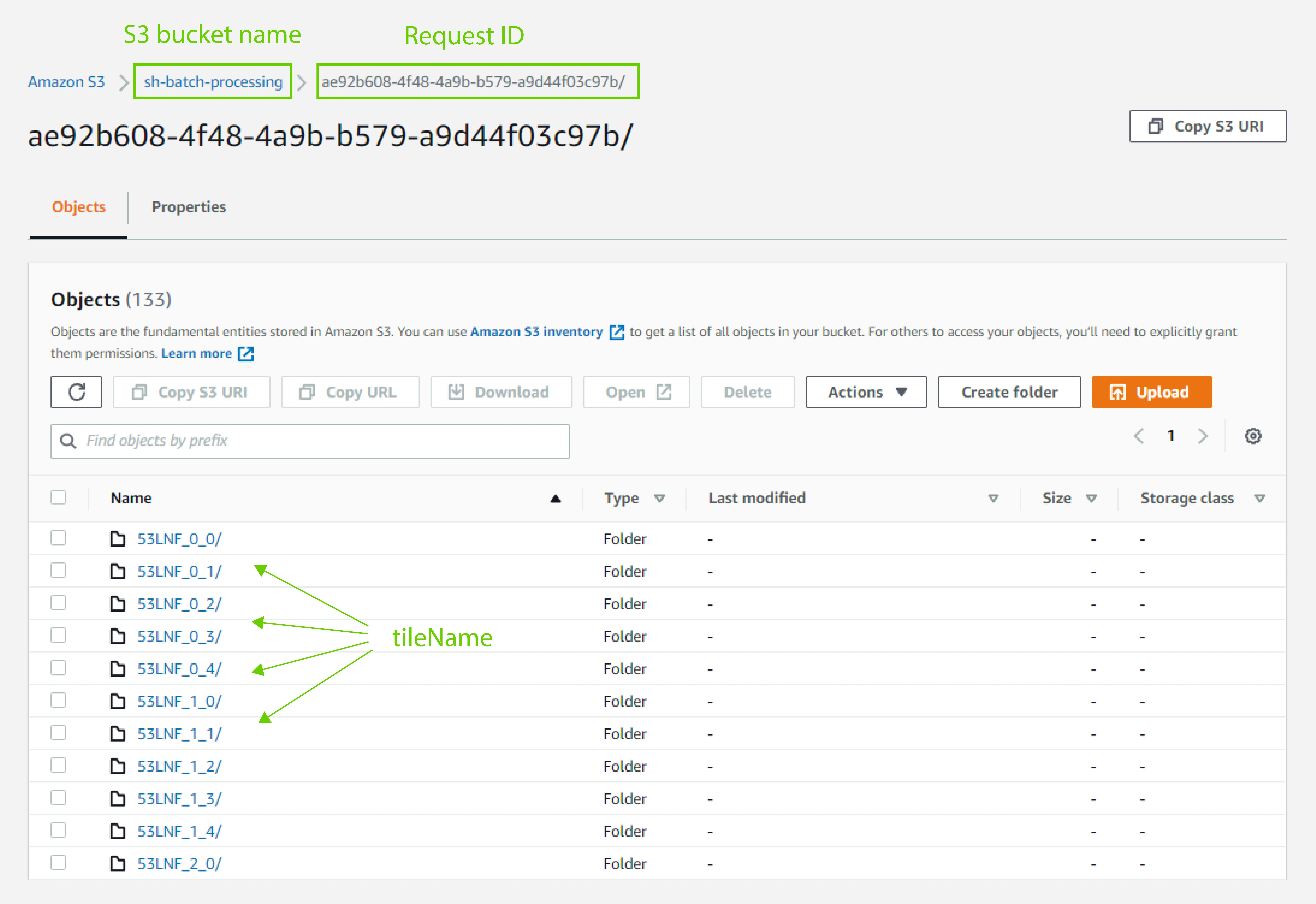
Caveat: If there was no data to process for this feature, the feature will still be marked with status `DONE` but with a '**No data**' message in the error column. * **FATAL**: Feature has failed X amount of times and will not be retried. The error column details the issue. --- Copy for LLM[View as Markdown](https://docs.planet.com/develop/apis/batch-processing/examples/) # Examples The requests below are written in Python. To execute them you need to create an OAuth client as is explained [here](https://docs.planet.com/develop/authentication.md#sentinel-hub-authentication). It is named `oauth` in these examples. ### Create a BatchV2 Processing Request #### Option 1: GeoTiff format output This request defines which data is requested and how it will be processed. In this example, we will calculate the maximum NDVI over two months for an area in Corsica and visualize the results using a built-in visualizer. The resulting image will be in a GeoTIFF format. To create a batch processing request, replace `{bucket}` with the name of your S3 bucket and run the following: * Python SDK ``` url = "https://services.sentinel-hub.com/batch/v2/process" evalscript = """ //VERSION=3 function setup() { return { input: [{ bands: ["B04", "B08"] }], output: [{ id: "default", bands: 3 }], mosaicking: Mosaicking.ORBIT } } function calcNDVI(sample) { var denom = sample.B04 + sample.B08 return ((denom != 0) ? (sample.B08 - sample.B04) / denom : 0.0) } const maxNDVIcolors = [ [-0.2, 0xbfbfbf], [0, 0xebebeb], [0.1, 0xc8c682], [0.2, 0x91bf52], [0.4, 0x4f8a2e], [0.6, 0x0f540c] ] const visualizer = new ColorRampVisualizer(maxNDVIcolors); function evaluatePixel(samples) { var max = 0 for (var i = 0; i < samples.length; i++) { var ndvi = calcNDVI(samples[i]) max = ndvi > max ? ndvi : max } ndvi = max return visualizer.process(ndvi) } """ payload = { "processRequest": { "input": { "bounds": { "bbox": [ 8.44, 41.31, 9.66, 43.1 ], "properties": { "crs": "http://www.opengis.net/def/crs/OGC/1.3/CRS84" } }, "data": [{ "dataFilter": { "timeRange": { "from": "2019-04-01T00:00:00Z", "to": "2019-06-30T00:00:00Z" }, "maxCloudCoverage": 70.0 }, "type": "sentinel-2-l2a" }] }, "output": { "responses": [{ "identifier": "default", "format": { "type": "image/tiff" } }] }, "evalscript": evalscript }, "input": { "type" : "tiling-grid", "id": 0, "resolution": 60.0 }, "output": { "type": "raster", "delivery": { "s3": { "url": "s3://{bucket}", "iamRoleARN": "{IAM-role-ARN}" } } }, "description": "Max NDVI over Corsica" } headers = { 'Content-Type': 'application/json' } response = oauth.request("POST", url, headers=headers, json = payload) response.json() ``` Extracting the batch request id from the response: * Python SDK ``` batch_request_id = response.json()['id'] ``` #### Option 2: Zarr format output In this example, we will calculate the maximum NDVI over two months for an area in Corsica. Besides the maximum NDVI, we will also return the values of bands B04 and B08, which were used to calculate the maximum NDVI. All three results will be stored as arrays in an output Zarr file. To create a batch processing request replace `{bucket}` with the name of your S3 bucket and run the following: * Python SDK ``` url = "https://services.sentinel-hub.com/batch/v2/process" evalscript = """ //VERSION=3 function setup() { return { input: [{ bands: ["B04", "B08"] }], output: [{ id: "maxNDVI", sampleType: "FLOAT32", bands: 1 }, { id: "band04", sampleType: "UINT16", bands: 1 }, { id: "band08", sampleType: "UINT16", bands: 1 }], mosaicking: Mosaicking.ORBIT } } function calcNDVI(sample) { var denom = sample.B04 + sample.B08 return ((denom != 0) ? (sample.B08 - sample.B04) / denom : 0.0) } function evaluatePixel(samples) { var maxNDVI = 0 var band04 = 0 var band08 = 0 for (var i = 0; i < samples.length; i++) { var ndvi = calcNDVI(samples[i]) if (ndvi > maxNDVI){ maxNDVI = ndvi band04 = samples[i].B04 band08 = samples[i].B08 } } return { maxNDVI: [maxNDVI], band04: [band04], band08: [band08] } } """ payload = { "processRequest": { "input": { "bounds": { "bbox": [ 8.44, 41.31, 9.66, 43.1 ], "properties": { "crs": "http://www.opengis.net/def/crs/OGC/1.3/CRS84" } }, "data": [ { "dataFilter": { "timeRange": { "from": "2019-04-01T00:00:00Z", "to": "2019-06-30T00:00:00Z" }, "maxCloudCoverage": 70 }, "type": "sentinel-2-l2a" } ] }, "output": { "responses": [ { "identifier": "band08", "format": { "type": "zarr/array" } }, { "identifier": "band04", "format": { "type": "zarr/array" } }, { "identifier": "maxNDVI", "format": { "type": "zarr/array" } } ] }, "evalscript": evalscript }, "input": { "type": "tiling-grid", "id": 6, "resolution": 100.0 }, "output": { "type": "zarr", "delivery": { "s3": { "url": "s3://{bucket}/{key}", "iamRoleARN": "{IAM-role-ARN}" } }, "group": { "zarr_format": 2 }, "arrayParameters": { "dtype": " max ? ndvi : max } ndvi = max return visualizer.process(ndvi) } """ payload = { "processRequest": { "input": { "bounds": { "bbox": [ 8.44, 41.31, 9.66, 43.1 ], "properties": { "crs": "http://www.opengis.net/def/crs/OGC/1.3/CRS84" } }, "data": [{ "dataFilter": { "timeRange": { "from": "2019-04-01T00:00:00Z", "to": "2019-06-30T00:00:00Z" }, "maxCloudCoverage": 70.0 }, "type": "sentinel-2-l2a" }] }, "output": { "responses": [{ "identifier": "default", "format": { "type": "image/tiff" } }] }, "evalscript": evalscript }, "input": { "type" : "geopackage", "features": { "s3": { "url": "s3://{bucket}/{path-to-geopackage}", "iamRoleARN": "{IAM-role-ARN}", } } }, "output": { "type": "raster", "delivery": { "s3": { "url": "s3://{bucket}", "iamRoleARN": "{IAM-role-ARN}" } } }, "description": "Max NDVI over Corsica" } headers = { 'Content-Type': 'application/json' } response = oauth.request("POST", url, headers=headers, json=payload) response.json() ``` #### Option 4: Google Storage Bucket Input and Delivery This example demonstrates how to use Google Cloud Storage buckets for both GeoPackage input and delivery of results. * Python SDK ``` url = "https://services.sentinel-hub.com/batch/v2/process" evalscript = """ //VERSION=3 function setup() { return { input: [{ bands: ["B04", "B08"] }], output: [{ id: "default", bands: 3 }], mosaicking: Mosaicking.ORBIT } } function calcNDVI(sample) { var denom = sample.B04 + sample.B08 return ((denom != 0) ? (sample.B08 - sample.B04) / denom : 0.0) } const maxNDVIcolors = [ [-0.2, 0xbfbfbf], [0, 0xebebeb], [0.1, 0xc8c682], [0.2, 0x91bf52], [0.4, 0x4f8a2e], [0.6, 0x0f540c] ] const visualizer = new ColorRampVisualizer(maxNDVIcolors); function evaluatePixel(samples) { var max = 0 for (var i = 0; i < samples.length; i++) { var ndvi = calcNDVI(samples[i]) max = ndvi > max ? ndvi : max } ndvi = max return visualizer.process(ndvi) } """ payload = { "processRequest": { "input": { "bounds": { "bbox": [ 8.44, 41.31, 9.66, 43.1 ], "properties": { "crs": "http://www.opengis.net/def/crs/OGC/1.3/CRS84" } }, "data": [{ "dataFilter": { "timeRange": { "from": "2019-04-01T00:00:00Z", "to": "2019-06-30T00:00:00Z" }, "maxCloudCoverage": 70.0 }, "type": "sentinel-2-l2a" }] }, "output": { "responses": [{ "identifier": "default", "format": { "type": "image/tiff" } }] }, "evalscript": evalscript }, "input": { "type" : "geopackage", "features": { "gs": { "url": "gs://{bucket}/{path-to-geopackage}", "credentials": "{base64-encoded-credentials}" } } }, "output": { "type": "raster", "delivery": { "gs": { "url": "gs://{bucket}/{key}", "credentials": "{base64-encoded-credentials}" } } }, "description": "Max NDVI over Corsica with Google Storage" } headers = { 'Content-Type': 'application/json' } response = oauth.request("POST", url, headers=headers, json=payload) response.json() ``` To prepare your Google Cloud Storage credentials, download your service account credentials in JSON format and encode them as base64: * CURL ``` cat my_creds.json | base64 ``` Replace `{base64-encoded-credentials}` with the output of this command in both the input and output sections of your request. ### Get Information About All of Your Batch Processing Requests * Python SDK ``` url = "https://services.sentinel-hub.com/batch/v2/process" response = oauth.request("GET", url) response.json() ``` ### Get Information About a Batch Processing Request * Python SDK ``` url = f"https://services.sentinel-hub.com/batch/v2/process/{batch_request_id}" response = oauth.request("GET", url) response.json() ``` ### Request Detailed Analysis (ANALYSE) * Python SDK ``` url = f"https://services.sentinel-hub.com/batch/v2/process/{batch_request_id}/analyse" response = oauth.request("POST", url) response.status_code ``` ### Request the Start of Processing (START) * Python SDK ``` url = f"https://services.sentinel-hub.com/batch/v2/process/{batch_request_id}/start" response = oauth.request("POST", url) response.status_code ``` ### Cancel a Batch Processing Request (STOP) * Python SDK ``` url = f"https://services.sentinel-hub.com/batch/v2/process/{batch_request_id}/stop" response = oauth.request("POST", url) response.status_code ``` --- Copy for LLM[View as Markdown](https://docs.planet.com/develop/apis/batch-processing/reference/) # Batch Processing API Reference * BatchV2 API * Process * postSubmit new batch processing request * getQuery batch process requests * getRetrieve a single batch process task by ID * putUpdate a batch process request * postRequest analysis of a batch process request * postStart (confirm) processing of a batch process request * postStop a batch process request * Tiling grid * getGet properties of all supported tiling grids * getGet properties of a single tiling grid [API docs by Redocly](https://redocly.com/redoc/) # API Reference (1.0.0) Download OpenAPI specification:[Download](https://docs.planet.com/redocusaurus/sh-prod-batchv2-api-spec.yaml) ## [](#tag/batch_v2_process)Process ## [](#tag/batch_v2_process/operation/createNewBatchV2ProcessingRequest)Submit new batch processing request ##### Authorizations: *OAuth2* ##### Request Body schema:application/jsonapplication/json | | | | ---------------------- | ---------------------------------------------------------------------------------------------------------- | | processRequestrequired | object (ProcessRequestForBatchV2)Batch processing equivalent of the [Process request](#operation/process). | | inputrequired | GeoPackageInput (object) or TilingGridInput (object) (BatchV2ProcessInput) | | outputrequired | RasterOutput (object) or ZarrOutput (object) (BatchV2ProcessOutput) | | description | stringOptional description that can be used to keep track of requests | ### Responses **201** Request submitted **400** Bad request **401** Unauthorized **403** Insufficient permissions post/batch/v2/process https\://services.sentinel-hub.com/batch/v2/process ### Request samples * Payload Content type application/jsonapplication/json Copy Expand all Collapse all `{ "processRequest": { "input": { "bounds": { "bbox": [ 13.822174072265625, 45.85080395917834, 14.55963134765625, 46.29191774991382 ], "geometry": { "type": "Polygon", "coordinates": [ [ [ 14.000701904296873, 46.23685258143992 ], [ 13.822174072265625, 46.09037664604301 ], [ 14.113311767578125, 45.85080395917834 ], [ 14.55963134765625, 46.038922598236 ], [ 14.441528320312498, 46.28717293114449 ], [ 14.17236328125, 46.29191774991382 ], [ 14.000701904296873, 46.23685258143992 ] ] ] }, "properties": { "crs": "http://www.opengis.net/def/crs/OGC/1.3/CRS84" } }, "data": [ { "type": "sentinel-2-l1c", "id": "string", "dataFilter": { "timeRange": { "from": "2018-10-01T00:00:00.000Z", "to": "2018-11-01T00:00:00.000Z" }, "mosaickingOrder": "mostRecent", "maxCloudCoverage": 100 }, "processing": { "upsampling": "NEAREST", "downsampling": "NEAREST", "harmonizeValues": true } } ] }, "output": { "responses": [ { "identifier": "", "format": { "type": "image/tiff" } } ] }, "evalscript": "string" }, "input": { "type": "geopackage", "features": { "s3": { "url": "string", "iamRoleARN": "string", "accessKey": "string", "secretAccessKey": "string", "region": "string" } }, "defaults": { "width": 512, "height": 512, "resolution": 0.1 } }, "output": { "type": "raster", "delivery": { "s3": { "url": "string", "iamRoleARN": "string", "accessKey": "string", "secretAccessKey": "string", "region": "string" } }, "overwrite": false, "skipExisting": false, "cogOutput": false, "cogParameters": { "overviewLevels": [ 0 ], "overviewMinSize": 0, "resamplingAlgorithm": "nearest", "blockxsize": 256, "blockysize": 256, "usePredictor": true }, "createCollection": false, "collectionId": "string" }, "description": "string" }` ### Response samples * 201 * 400 Content type application/json Copy Expand all Collapse all `{ "id": "497f6eca-6276-4993-bfeb-53cbbbba6f08", "request": { "processRequest": { "input": { "bounds": { "bbox": [ 13.822174072265625, 45.85080395917834, 14.55963134765625, 46.29191774991382 ], "geometry": { "type": "Polygon", "coordinates": [ [ [ 14.000701904296873, 46.23685258143992 ], [ 13.822174072265625, 46.09037664604301 ], [ 14.113311767578125, 45.85080395917834 ], [ 14.55963134765625, 46.038922598236 ], [ 14.441528320312498, 46.28717293114449 ], [ 14.17236328125, 46.29191774991382 ], [ 14.000701904296873, 46.23685258143992 ] ] ] }, "properties": { "crs": "http://www.opengis.net/def/crs/OGC/1.3/CRS84" } }, "data": [ { "type": "sentinel-2-l1c", "id": "string", "dataFilter": { "timeRange": { "from": "2018-10-01T00:00:00.000Z", "to": "2018-11-01T00:00:00.000Z" }, "mosaickingOrder": "mostRecent", "maxCloudCoverage": 100 }, "processing": { "upsampling": "NEAREST", "downsampling": "NEAREST", "harmonizeValues": true } } ] }, "output": { "responses": [ { "identifier": "", "format": { "type": "image/tiff" } } ] }, "evalscript": "string" }, "input": { "type": "geopackage", "features": { "s3": { "url": "string", "iamRoleARN": "string", "accessKey": "string", "secretAccessKey": "string", "region": "string" } }, "defaults": { "width": 512, "height": 512, "resolution": 0.1 } }, "output": { "type": "raster", "delivery": { "s3": { "url": "string", "iamRoleARN": "string", "accessKey": "string", "secretAccessKey": "string", "region": "string" } }, "overwrite": false, "skipExisting": false, "cogOutput": false, "cogParameters": { "overviewLevels": [ 0 ], "overviewMinSize": 0, "resamplingAlgorithm": "nearest", "blockxsize": 256, "blockysize": 256, "usePredictor": true }, "createCollection": false, "collectionId": "string" }, "description": "string" }, "domainAccountId": "4e1699b2-af74-455a-818d-6f1ec31a6d19", "projectId": "5a8591dd-4039-49df-9202-96385ba3eff8", "workspaceId": "ef0efa32-d1c1-43d4-a5e2-fe7b4f00403c", "status": "CREATED", "error": "string", "userAction": "NONE", "userActionUpdated": "2019-08-24T14:15:22Z", "created": "2019-08-24T14:15:22Z", "completionPercentage": 0, "lastUpdated": "2019-08-24T14:15:22Z", "costPU": 0, "costMC": 0, "stoppedStatusReason": "OUT_OF_PU" }` ## [](#tag/batch_v2_process/operation/getAllBatchV2ProcessRequests)Query batch process requests ##### Authorizations: *OAuth2* ##### query Parameters | | | | --------- | -------------------------------------------------------------------------------------------------------------------------------------------------------------------------------------------------------------------------------------------------------------------------------------------------------------------- | | count | integer \Upper limit to the number of items to retrieve. It cannot be larger than the endpoint-specific limit. If omitted, the endpoint-specific limit is used. For more records, use *viewtoken* to page through. | | viewtoken | stringWhen the total number of items is larger than *count*, the response contains *viewtoken*. This *viewtoken* can be used in the next request to retrieve the next page of items.The next page can be retrieved by repeating the query. However, replace your URL with the next URL in the returned links object. | | sort | stringEnum: "created" "created:desc" "status" "status:desc"Sort the batch process requests by given field. Omit for default ordering. | ### Responses **200** Successful response **401** Unauthorized **403** Insufficient permissions get/batch/v2/process https\://services.sentinel-hub.com/batch/v2/process ### Response samples * 200 Content type application/json Copy Expand all Collapse all `{ "data": [ { "id": "497f6eca-6276-4993-bfeb-53cbbbba6f08", "request": { "processRequest": { "input": { "bounds": { "bbox": [ 13.822174072265625, 45.85080395917834, 14.55963134765625, 46.29191774991382 ], "geometry": { "type": "Polygon", "coordinates": [ [ [ 14.000701904296873, 46.23685258143992 ], [ 13.822174072265625, 46.09037664604301 ], [ 14.113311767578125, 45.85080395917834 ], [ 14.55963134765625, 46.038922598236 ], [ 14.441528320312498, 46.28717293114449 ], [ 14.17236328125, 46.29191774991382 ], [ 14.000701904296873, 46.23685258143992 ] ] ] }, "properties": { "crs": "http://www.opengis.net/def/crs/OGC/1.3/CRS84" } }, "data": [ { "type": "sentinel-2-l1c", "id": "string", "dataFilter": { "timeRange": { "from": "2018-10-01T00:00:00.000Z", "to": "2018-11-01T00:00:00.000Z" }, "mosaickingOrder": "mostRecent", "maxCloudCoverage": 100 }, "processing": { "upsampling": "NEAREST", "downsampling": "NEAREST", "harmonizeValues": true } } ] }, "output": { "responses": [ { "identifier": "", "format": { "type": "image/tiff" } } ] }, "evalscript": "string" }, "input": { "type": "geopackage", "features": { "s3": { "url": "string", "iamRoleARN": "string", "accessKey": "string", "secretAccessKey": "string", "region": "string" } }, "defaults": { "width": 512, "height": 512, "resolution": 0.1 } }, "output": { "type": "raster", "delivery": { "s3": { "url": "string", "iamRoleARN": "string", "accessKey": "string", "secretAccessKey": "string", "region": "string" } }, "overwrite": false, "skipExisting": false, "cogOutput": false, "cogParameters": { "overviewLevels": [ 0 ], "overviewMinSize": 0, "resamplingAlgorithm": "nearest", "blockxsize": 256, "blockysize": 256, "usePredictor": true }, "createCollection": false, "collectionId": "string" }, "description": "string" }, "domainAccountId": "4e1699b2-af74-455a-818d-6f1ec31a6d19", "projectId": "5a8591dd-4039-49df-9202-96385ba3eff8", "workspaceId": "ef0efa32-d1c1-43d4-a5e2-fe7b4f00403c", "status": "CREATED", "error": "string", "userAction": "NONE", "userActionUpdated": "2019-08-24T14:15:22Z", "created": "2019-08-24T14:15:22Z", "completionPercentage": 0, "lastUpdated": "2019-08-24T14:15:22Z", "costPU": 0, "costMC": 0, "stoppedStatusReason": "OUT_OF_PU" } ], "links": { "currentToken": "string", "nextToken": "string", "previousToken": "string", "@id": "http://example.com", "next": "http://example.com", "previous": "http://example.com" } }` ## [](#tag/batch_v2_process/operation/getSingleBatchV2ProcessTaskById)Retrieve a single batch process task by ID ##### Authorizations: *OAuth2* ##### path Parameters | | | | -------------- | --------------------- | | taskIdrequired | string \Task ID | ### Responses **200** Successful response **401** Unauthorized **403** Insufficient permissions **404** Not found get/batch/v2/process/{taskId} https\://services.sentinel-hub.com/batch/v2/process/{taskId} ### Response samples * 200 * 404 Content type application/json Copy Expand all Collapse all `{ "id": "497f6eca-6276-4993-bfeb-53cbbbba6f08", "request": { "processRequest": { "input": { "bounds": { "bbox": [ 13.822174072265625, 45.85080395917834, 14.55963134765625, 46.29191774991382 ], "geometry": { "type": "Polygon", "coordinates": [ [ [ 14.000701904296873, 46.23685258143992 ], [ 13.822174072265625, 46.09037664604301 ], [ 14.113311767578125, 45.85080395917834 ], [ 14.55963134765625, 46.038922598236 ], [ 14.441528320312498, 46.28717293114449 ], [ 14.17236328125, 46.29191774991382 ], [ 14.000701904296873, 46.23685258143992 ] ] ] }, "properties": { "crs": "http://www.opengis.net/def/crs/OGC/1.3/CRS84" } }, "data": [ { "type": "sentinel-2-l1c", "id": "string", "dataFilter": { "timeRange": { "from": "2018-10-01T00:00:00.000Z", "to": "2018-11-01T00:00:00.000Z" }, "mosaickingOrder": "mostRecent", "maxCloudCoverage": 100 }, "processing": { "upsampling": "NEAREST", "downsampling": "NEAREST", "harmonizeValues": true } } ] }, "output": { "responses": [ { "identifier": "", "format": { "type": "image/tiff" } } ] }, "evalscript": "string" }, "input": { "type": "geopackage", "features": { "s3": { "url": "string", "iamRoleARN": "string", "accessKey": "string", "secretAccessKey": "string", "region": "string" } }, "defaults": { "width": 512, "height": 512, "resolution": 0.1 } }, "output": { "type": "raster", "delivery": { "s3": { "url": "string", "iamRoleARN": "string", "accessKey": "string", "secretAccessKey": "string", "region": "string" } }, "overwrite": false, "skipExisting": false, "cogOutput": false, "cogParameters": { "overviewLevels": [ 0 ], "overviewMinSize": 0, "resamplingAlgorithm": "nearest", "blockxsize": 256, "blockysize": 256, "usePredictor": true }, "createCollection": false, "collectionId": "string" }, "description": "string" }, "domainAccountId": "4e1699b2-af74-455a-818d-6f1ec31a6d19", "projectId": "5a8591dd-4039-49df-9202-96385ba3eff8", "workspaceId": "ef0efa32-d1c1-43d4-a5e2-fe7b4f00403c", "status": "CREATED", "error": "string", "userAction": "NONE", "userActionUpdated": "2019-08-24T14:15:22Z", "created": "2019-08-24T14:15:22Z", "completionPercentage": 0, "lastUpdated": "2019-08-24T14:15:22Z", "costPU": 0, "costMC": 0, "stoppedStatusReason": "OUT_OF_PU" }` ## [](#tag/batch_v2_process/operation/updateBatchV2ProcessRequest)Update a batch process request Only the requests that are not currently being processed nor waiting to be processed can be updated. ##### Authorizations: *OAuth2* ##### path Parameters | | | | -------------- | --------------------- | | taskIdrequired | string \Task ID | ##### Request Body schema: application/json | | | | ----------- | ----------------------------------------------------------------------------------------------------------------------- | | description | stringOptional description that can be used to keep track of requests. If omitted, the description will not be changed. | ### Responses **200** Successful response **400** Unauthorized **401** Unauthorized **403** Insufficient permissions **404** Not found **409** Conflict in the request put/batch/v2/process/{taskId} https\://services.sentinel-hub.com/batch/v2/process/{taskId} ### Request samples * Payload Content type application/json Copy `{ "description": "string" }` ### Response samples * 200 * 404 * 409 Content type application/json Copy Expand all Collapse all `{ "processRequest": { "input": { "bounds": { "bbox": [ 13.822174072265625, 45.85080395917834, 14.55963134765625, 46.29191774991382 ], "geometry": { "type": "Polygon", "coordinates": [ [ [ 14.000701904296873, 46.23685258143992 ], [ 13.822174072265625, 46.09037664604301 ], [ 14.113311767578125, 45.85080395917834 ], [ 14.55963134765625, 46.038922598236 ], [ 14.441528320312498, 46.28717293114449 ], [ 14.17236328125, 46.29191774991382 ], [ 14.000701904296873, 46.23685258143992 ] ] ] }, "properties": { "crs": "http://www.opengis.net/def/crs/OGC/1.3/CRS84" } }, "data": [ { "type": "sentinel-2-l1c", "id": "string", "dataFilter": { "timeRange": { "from": "2018-10-01T00:00:00.000Z", "to": "2018-11-01T00:00:00.000Z" }, "mosaickingOrder": "mostRecent", "maxCloudCoverage": 100 }, "processing": { "upsampling": "NEAREST", "downsampling": "NEAREST", "harmonizeValues": true } } ] }, "output": { "responses": [ { "identifier": "", "format": { "type": "image/tiff" } } ] }, "evalscript": "string" }, "input": { "type": "geopackage", "features": { "s3": { "url": "string", "iamRoleARN": "string", "accessKey": "string", "secretAccessKey": "string", "region": "string" } }, "defaults": { "width": 512, "height": 512, "resolution": 0.1 } }, "output": { "type": "raster", "delivery": { "s3": { "url": "string", "iamRoleARN": "string", "accessKey": "string", "secretAccessKey": "string", "region": "string" } }, "overwrite": false, "skipExisting": false, "cogOutput": false, "cogParameters": { "overviewLevels": [ 0 ], "overviewMinSize": 0, "resamplingAlgorithm": "nearest", "blockxsize": 256, "blockysize": 256, "usePredictor": true }, "createCollection": false, "collectionId": "string" }, "description": "string" }` ## [](#tag/batch_v2_process/operation/batchV2Analyse)Request analysis of a batch process request ##### Authorizations: *OAuth2* ##### path Parameters | | | | -------------- | --------------------- | | taskIdrequired | string \Task ID | ### Responses **204** Success **400** Bad request **401** Unauthorized **403** Insufficient permissions **404** Not found post/batch/v2/process/{taskId}/analyse https\://services.sentinel-hub.com/batch/v2/process/{taskId}/analyse ### Response samples * 400 * 404 Content type application/json Copy Expand all Collapse all `{ "error": { "status": 0, "reason": "string", "message": "string", "code": "COMMON_BAD_PAYLOAD", "errors": { } } }` ## [](#tag/batch_v2_process/operation/batchV2StartProcessRequest)Start (confirm) processing of a batch process request ##### Authorizations: *OAuth2* ##### path Parameters | | | | -------------- | --------------------- | | taskIdrequired | string \Task ID | ### Responses **204** Success **400** Bad request **401** Unauthorized **403** Insufficient permissions **404** Not found post/batch/v2/process/{taskId}/start https\://services.sentinel-hub.com/batch/v2/process/{taskId}/start ### Response samples * 400 * 404 Content type application/json Copy Expand all Collapse all `{ "error": { "status": 0, "reason": "string", "message": "string", "code": "COMMON_BAD_PAYLOAD", "errors": { } } }` ## [](#tag/batch_v2_process/operation/batchV2StopProcessRequest)Stop a batch process request ##### Authorizations: *OAuth2* ##### path Parameters | | | | -------------- | --------------------- | | taskIdrequired | string \Task ID | ### Responses **204** Success **400** Bad request **401** Unauthorized **403** Insufficient permissions **404** Not found post/batch/v2/process/{taskId}/stop https\://services.sentinel-hub.com/batch/v2/process/{taskId}/stop ### Response samples * 400 * 404 Content type application/json Copy Expand all Collapse all `{ "error": { "status": 0, "reason": "string", "message": "string", "code": "COMMON_BAD_PAYLOAD", "errors": { } } }` ## [](#tag/batch_v2_tiling_grid)Tiling grid ## [](#tag/batch_v2_tiling_grid/operation/getBatchV2TilingGridsProperties)Get properties of all supported tiling grids ##### Authorizations: *OAuth2* ##### query Parameters | | | | --------- | -------------------------------------------------------------------------------------------------------------------------------------------------------------------------------------------------------------------------------------------------------------------------------------------------------------------- | | count | integer \Upper limit to the number of items to retrieve. It cannot be larger than the endpoint-specific limit. If omitted, the endpoint-specific limit is used. For more records, use *viewtoken* to page through. | | viewtoken | stringWhen the total number of items is larger than *count*, the response contains *viewtoken*. This *viewtoken* can be used in the next request to retrieve the next page of items.The next page can be retrieved by repeating the query. However, replace your URL with the next URL in the returned links object. | ### Responses **200** Successful response **401** Unauthorized get/batch/v2/tilinggrids https\://services.sentinel-hub.com/batch/v2/tilinggrids ### Response samples * 200 Content type application/json Copy Expand all Collapse all `{ "data": [ { "id": 0, "name": "string", "properties": { "tileWidth": 0.1, "tileHeight": 0.1, "resolutions": [ 0.1 ], "unit": "METRE" } } ], "links": { "currentToken": "string", "nextToken": "string", "previousToken": "string", "@id": "http://example.com", "next": "http://example.com", "previous": "http://example.com" } }` ## [](#tag/batch_v2_tiling_grid/operation/getBatchV2TilingGridProperties)Get properties of a single tiling grid ##### Authorizations: *OAuth2* ##### path Parameters | | | | ---------- | ------------------------------ | | idrequired | integer \Tilinggrids ID | ### Responses **200** Successful response **400** Bad request **401** Unauthorized get/batch/v2/tilinggrids/{id} https\://services.sentinel-hub.com/batch/v2/tilinggrids/{id} ### Response samples * 200 * 400 Content type application/json Copy Expand all Collapse all `{ "id": 0, "name": "string", "properties": { "tileWidth": 0.1, "tileHeight": 0.1, "resolutions": [ 0.1 ], "unit": "METRE" } }` --- Copy for LLM[View as Markdown](https://docs.planet.com/develop/apis/batch-statistical/) # Batch Statistical API Requires Enterprise License The Batch Statistical API is only available for users on enterprise plans. If you do not have an enterprise plan, and would like to try it out, [contact us](https://www.planet.com/contact-sales) or [upgrade](https://www.planet.com/pricing/?tab=platform). The Batch Statistical API enables you to request statistics similarly to the [Statistical API](https://docs.planet.com/develop/apis/statistical.md), but for multiple polygons at once and/or for longer aggregations. A typical use case would be calculating statistics for all parcels in a country. Similar to the [Batch Processing API](https://docs.planet.com/develop/apis/batch-processing.md), this is an asynchronous REST service. This means that data will not be immediately returned in the response of the request but delivered to your object storage, which needs to be specified in the request. You can find more details about the API in the [API Reference](https://docs.planet.com/develop/apis/batch-statistical/reference.md) or in the [examples](https://docs.planet.com/develop/apis/batch-statistical/examples.md) of the workflow. ## Deployments | Deployment | API endpoint | Region | | ------------------ | ------------------------------------------------------- | ------------ | | AWS EU (Frankfurt) | | eu-central-1 | ## Rate Limiting The Batch Statistical API follows the general rate limiting policies described in [Rate Limiting](https://docs.planet.com/develop/rate-limiting.md). Rate limits are in place for service protection and should not affect normal usage. ## Data Sources Restrictions All data sources must be from the same deployment where the request is made. ## Workflow The Batch Statistical API workflow in many ways resembles the [Batch Processing API workflow](https://docs.planet.com/develop/apis/batch-processing.md#workflow). Available actions and statuses are: * user's actions: `ANALYSE`, `START` and `STOP`. * request statuses: `CREATED`, `ANALYSING`, `ANALYSIS_DONE`, `STOPPED`, `PROCESSING`, `DONE`, and `FAILED`. The Batch Statistical API comes with a set of REST actions that support the execution of various steps in the workflow. The diagram below shows all possible statuses of the Batch Statistical request and users' actions that trigger transitions among them. The workflow starts when you post a new Batch Statistical request. In this step, the system: * creates a new Batch Statistical request with status `CREATED`, * validates your input (not the evalscript), * returns the overview of the created request. You can then decide to either request an additional analysis of the request or start the processing. When an additional analysis is requested: * the status of the request changes to `ANALYSING`, * the evalscript is validated, * After the analysis is finished, the status of the request changes to `ANALYSIS_DONE`. If you choose to start processing directly, the system still executes the analysis, but when the analysis is done, it automatically starts processing. This is not explicitly shown in the diagram to keep it simple. When you start the processing: * the status of the request changes to `PROCESSING` (this may take a while), * the processing starts, * spent processing units are billed periodically. When the processing finishes, the status of the request changes to `DONE`. #### Stopping the request A request might be stopped for the following reasons: * it is requested by a user (user action) * user is out of processing units (see chapter below) * something is wrong with the processing of the request A user may stop the request in the following states: `ANALYSING`, `ANALYSIS_DONE`, and `PROCESSING`. However: * if the status is `ANALYSING`, the analysis will complete * if the status is `PROCESSING`, all features (polygons) that have been processed or are being processed at that moment are charged for * you are not allowed to restart the request in the next 30 minutes The service itself may also stop the request when processing of a lot of features is repeatedly failing. `stoppedStatusReason` of such requests will be `UNHEALTHY`. This can happen if the service is unstable or if something is wrong with the request. If the former, the request should eventually be restarted by our team. #### Processing unit costs To create, analyse, or initiate a request, the user must have at least 1000 processing units available in their account. If available processing units of a user drop below `1000` while the request is being processed, the request is automatically stopped and cannot be restarted in the next 60 minutes. Therefore, it is highly recommended to start a request with a sufficient reserve. More information about batch statistical costs is available [here](https://docs.planet.com/platform/processing-units.md#batch-statistical-api). #### Automatic deletion of stale data Stale (inactive) requests will be deleted after a specific period of inactivity, depending on their status: * requests with status `CREATED` are deleted after 7 days of inactivity * requests with status `FAILED` are deleted after 15 days of inactivity * all other requests are deleted after 30 days of inactivity note Note that only such requests themselves will be deleted, while the requests' result (created statistics) will remain under your control in your object storage bucket. ## Input Polygons as a GeoPackage File The Batch Statistical API accepts a [GeoPackage file](https://www.geopackage.org/) containing features (polygons) as an input. The GeoPackage must be stored in your object storage and must be accessible to the service for reading (find more details about this in the [object storage configuration](#object-storage-configuration) section below). In a batch statistical request, the input GeoPackage is specified by setting the path to the `.gpkg` file in the `input.features.s3` or `input.features.gs` parameter. All features (polygons) in an input GeoPackage must be in the same CRS [supported by us](https://docs.planet.com/develop/apis/processing.md#crs-support). There can be a maximum of 700,000 features in the GeoPackage. ## Evalscript and Batch Statistical API The exact specifics as described for [evalscript and Statistical API](https://docs.planet.com/develop/apis/statistical.md#statistical-api-and-evalscripts) also apply to the Batch Statistical API. Evalscripts smaller than 32KB in size can be provided directly in a batch statistical request under `evalscript` parameter. If your evalscript exceeds this limit, you can store it in your object storage bucket and provide a reference to it in a batch statistical request under the `evalscriptReference` parameter. ## Processing Results Outputs of a Batch Statistical API request are JSON files stored in your object storage. Each `.json` file will contain the requested statistics for one feature (polygon) in the provided GeoPackage. You can connect statistics in a JSON file with the corresponding feature (polygon) in the GeoPackage based on: * `id` of a feature from GeoPackage is used as the name of the JSON file (for example, `1.json`, `2.json`) and available in the JSON file as `id` property OR * a custom column `identifier` of type string can be added to GeoPackage and its value will be available in json file as `identifier` property The outputs will be stored in the bucket and the folder specified by `output.s3.url` or `output.gs.url` parameter of the batch statistical request. The URL supports templating with placeholders like ``, ``, and `` to customize output file organization (see [API Reference](https://docs.planet.com/develop/apis/batch-statistical/reference.md) for details). The outputs will be available in a sub-folder named after the ID of your request (for example, `s3://{bucket}/{my-folder}/db7de265-dfd4-4dc0-bc82-74866078a5ce`). ## Object Storage Configuration The Batch Statistical API requires access to object storage for reading input data and storing processing results. We support two object storage providers: * **Amazon S3** * **Google Cloud Storage (GCS)** ### Supported Use Cases Object storage is used for: * Reading GeoPackage files with input features (polygons) * Reading evalscript files (optional, evalscripts can also be provided directly in the request) * Uploading processing results (JSON files with statistics) One bucket or different buckets can be used for all three purposes. ### AWS S3 Configuration The Batch Statistical API supports two authentication methods for AWS S3. **We recommend using the IAM Assume Role method** for enhanced security and fine-grained access control. #### Authentication Methods ##### Option 1: IAM Assume Role (Recommended) The IAM Assume Role method provides better security by allowing temporary credentials and fine-grained access control without exposing long-term credentials. To use this method, provide the ARN of an IAM role that has access to your S3 bucket: ``` { "output": { "s3": { "url": "s3://{bucket}/{key}", "region": "{region}", "iamRoleARN": "{IAM-role-ARN}" } } } ``` **Setup Steps:** 1. **Create an IAM Policy for S3 Access** Create a policy that grants the necessary permissions to your S3 bucket: ``` { "Version": "2012-10-17", "Statement": [ { "Effect": "Allow", "Action": [ "s3:GetObject", "s3:PutObject", "s3:DeleteObject", "s3:ListBucket" ], "Resource": ["arn:aws:s3:::{bucket}", "arn:aws:s3:::{bucket}/*"] } ] } ``` 2. **Create an IAM Role** * In the AWS IAM console, create a new role * Choose "AWS account" as the trusted entity type * Select "Another AWS account" and enter account ID: `614251495211` * Attach the policy created in step 1 * Note the Role ARN for use in your API requests 3. **Configure Trust Relationship (Optional but Recommended)** For additional security, modify the role's trust policy: ``` { "Version": "2012-10-17", "Statement": [ { "Effect": "Allow", "Principal": { "AWS": "arn:aws:iam::614251495211:root" }, "Action": "sts:AssumeRole", "Condition": { "StringEquals": { "sts:ExternalId": "{domain-account-id}" }, "StringLike": { "sts:RoleSessionName": "sentinelhub" } } } ] } ``` Replace `{domain-account-id}` with your domain account ID from the [Dashboard](https://insights.planet.com/account/#/). ##### Option 2: Access Key & Secret Key Alternatively, you can provide AWS access credentials directly: ``` { "output": { "s3": { "url": "s3://{bucket}/{key}", "accessKey": "{access-key}", "secretAccessKey": "{secret-access-key}", "region": "{region}" } } } ``` The access key and secret must be linked to an IAM user with the following permissions on your S3 bucket: * `s3:GetObject` * `s3:PutObject` * `s3:DeleteObject` * `s3:ListBucket` To create access keys, see the [AWS documentation on programmatic access](https://docs.aws.amazon.com/general/latest/gr/aws-sec-cred-types.html). #### Using S3 Configuration in Requests The S3 configuration can be used in: * `input.features.s3` - to specify the bucket where the GeoPackage file is available (required) * `evalscriptReference.s3` - to specify the bucket where the evalscript .js file is available (optional) * `output.s3` - to specify the bucket where the results will be stored (required) Check [Batch Statistical API reference](https://docs.planet.com/develop/apis/batch-statistical/reference.md) for more information. ### Google Cloud Storage Configuration Google Cloud Storage is supported for GeoPackage input, evalscript input, and output delivery. Authentication requires a service account with base64-encoded credentials. #### Preparing Credentials 1. Download your service account credentials in JSON format (not P12) 2. Encode them as a base64 string: ``` cat my_creds.json | base64 ``` #### Using GCS for Input To read a GeoPackage or evalscript from Google Cloud Storage: ``` { "input": { "features": { "gs": { "url": "gs://{bucket}/{key}", "credentials": "{base64-encoded-credentials}" } } } } ``` #### Using GCS for Output To deliver results to Google Cloud Storage: ``` { "output": { "gs": { "url": "gs://{bucket}/{key}", "credentials": "{base64-encoded-credentials}" } } } ``` #### Required GCS Permissions The service account must have the following permissions on the specified bucket: * `storage.objects.create` * `storage.objects.get` * `storage.objects.delete` * `storage.objects.list` These permissions can be granted through IAM roles such as `Storage Object Admin` or custom roles. If possible, restrict access to the specific delivery path within the bucket for enhanced security. ### Cross-Cloud and Cross-Region Support The Batch Statistical API provides complete flexibility in choosing storage locations for both input and output. Surcharges apply based on where your **processing results are delivered** (output storage location). #### Storage Configuration Options The table below shows output storage options for each deployment and their associated costs. Surcharges apply only to the volume of output data transferred to your storage. **Important:** Input and output storage can be configured independently - you can mix and match any combination. For example, you can read input from GCS and write output to S3, or read from S3 in one region and write to S3 in another region. Input storage location does not affect costs. | Deployment | Region | Output Storage Location | Additional PU Cost | | ------------------ | ------------ | ----------------------- | ------------------ | | AWS EU (Frankfurt) | eu-central-1 | S3 eu-central-1 | None | | AWS EU (Frankfurt) | eu-central-1 | S3 (any other region) | 0.03 PU/MB | | AWS EU (Frankfurt) | eu-central-1 | Google Cloud Storage | 0.1 PU/MB | **Output Data Transfer Surcharges Summary:** * Cross-region (same cloud): 0.03 PU per MB * Cross-cloud: 0.1 PU per MB **Important Notes:** * Surcharges apply only to output data transfer (processing results) * Input location (GeoPackage and evalscript files) does not affect costs * When using an AWS S3 bucket in a different region than the deployment, specify the `region` parameter in your request: ``` { "output": { "s3": { "url": "s3://{bucket}/{key}", "region": "{region}", "iamRoleARN": "{IAM-role-ARN}" } } } ``` --- Copy for LLM[View as Markdown](https://docs.planet.com/develop/apis/batch-statistical/examples/) # Examples of Batch Statistical Workflow The requests below are written in Python. To execute them, you need to create an OAuth client as is explained [here](https://docs.planet.com/develop/authentication.md#sentinel-hub-authentication). It is named `oauth` in these examples. ## Create a Batch Statistical Request This request defines which data is requested and how it will be processed. In this example, we will receive the statistics for a single band on a given day. To create a batch statistical request, replace the `input.features.s3.url` field with the actual path to the GeoPackage features, and the `output.s3.url` field with the desired path where the output data will be processed. * Python SDK ``` evalscript = """ //VERSION=3 function setup() { return { input: [{ bands: [ "B04", "dataMask" ] }], output: [ { id: "output_B04", bands: 1, sampleType: "FLOAT32" }, { id: "dataMask", bands: 1 }] } } function evaluatePixel(samples) { return { output_B04: [samples.B04], dataMask: [samples.dataMask] } } """ request_payload = { "input": { "features":{ "s3": { "url": "s3://{bucket}/{path-to-geopackage}", "accessKey": "{access-key}, "secretAccessKey": "{secret-access-key} } }, "data": [ { "type": "sentinel-2-l2a", "dataFilter": { "mosaickingOrder": "leastCC" } } ] }, "aggregation": { "timeRange": { "from": "2020-06-01T00:00:00Z", "to": "2020-07-31T00:00:00Z" }, "aggregationInterval": { "of": "P30D" }, "evalscript": evalscript, "resx": 10, "resy": 10 }, "output": { "s3": { "url": "s3://{bucket}/{key}", "accessKey": "{access-key}, "secretAccessKey": "{secret-access-key} } } } headers = { 'Content-Type': 'application/json', 'Accept': 'application/json' } url = "https://services.sentinel-hub.com/statistics/batch/v1" response = oauth.request("POST", url=url, headers=headers, json=request_payload) request_id = response.json()['id'] ``` Note that in the above example, we are specifying an `accessKey` and `secretAccessKey`, so we can read and write to the user's bucket. You can find more details about this under the [Object Storage Configuration section](https://docs.planet.com/develop/apis/batch-statistical.md#object-storage-configuration). ## Create a Batch Statistical Request with Google Storage This example demonstrates how to use Google Cloud Storage for both GeoPackage input and delivery of results instead of S3. * Python SDK ``` evalscript = """ //VERSION=3 function setup() { return { input: [{ bands: [ "B04", "dataMask" ] }], output: [ { id: "output_B04", bands: 1, sampleType: "FLOAT32" }, { id: "dataMask", bands: 1 }] } } function evaluatePixel(samples) { return { output_B04: [samples.B04], dataMask: [samples.dataMask] } } """ request_payload = { "input": { "features":{ "gs": { "url": "gs://{bucket}/{path-to-geopackage}", "credentials": "{base64-encoded-credentials}" } }, "data": [ { "type": "sentinel-2-l2a", "dataFilter": { "mosaickingOrder": "leastCC" } } ] }, "aggregation": { "timeRange": { "from": "2020-06-01T00:00:00Z", "to": "2020-07-31T00:00:00Z" }, "aggregationInterval": { "of": "P30D" }, "evalscript": evalscript, "resx": 10, "resy": 10 }, "output": { "gs": { "url": "gs://{bucket}/{key}", "credentials": "{base64-encoded-credentials}" } } } headers = { 'Content-Type': 'application/json', 'Accept': 'application/json' } url = "https://services.sentinel-hub.com/statistics/batch/v1" response = oauth.request("POST", url=url, headers=headers, json=request_payload) request_id = response.json()['id'] ``` To prepare your Google Cloud Storage credentials, download your service account credentials in JSON format and encode them as base64: * CURL ``` cat my_creds.json | base64 ``` Replace `{base64-encoded-credentials}` with the output of this command in both the input and output sections of your request. ### Get Information About a Batch Statistical Request * Python SDK ``` response = oauth.request("GET", f"https://services.sentinel-hub.com/statistics/batch/v1/{request_id}") response.json() ``` ### Get Status Information About a Batch Statistical Request * Python SDK ``` response = oauth.request("GET", f"https://services.sentinel-hub.com/statistics/batch/v1/{request_id}/status") response.json() ``` ### Request Analysis of a Batch Statistical Request (ANALYSIS) * Python SDK ``` response = oauth.request("POST", f"https://services.sentinel-hub.com/statistics/batch/v1/{request_id}/analyse") response.status_code ``` ### Request the Start of a Batch Statistical Request (START) * Python SDK ``` response = oauth.request("POST", f"https://services.sentinel-hub.com/statistics/batch/v1/{request_id}/start") response.status_code ``` ### Stop a Batch Statistical Request (STOP) * Python SDK ``` response = oauth.request("POST", f"https://services.sentinel-hub.com/statistics/batch/v1/{request_id}/stop") response.status_code ``` --- Copy for LLM[View as Markdown](https://docs.planet.com/develop/apis/batch-statistical/reference/) # Batch Statistical API Reference * Batch Stats API * Statistical * postSubmit a new statistical batch request * getQuery statistical batch requests * getRetrieve a single batch statistical request * getRetrieve the status of a batch statistical request. * postRequest analysis of a batch statistical request * postStart (confirm) processing of a batch statistical request * postStop a batch statistical request [API docs by Redocly](https://redocly.com/redoc/) # API Reference (1.0.0) Download OpenAPI specification:[Download](https://docs.planet.com/redocusaurus/sh-prod-batch-statistical-api-spec.yaml) ## [](#tag/batch_statistical)Statistical ## [](#tag/batch_statistical/operation/createNewBatchStatisticsRequest)Submit a new statistical batch request ##### Authorizations: *OAuth2* ##### Request Body schema:application/jsonapplication/json | | | | ------------------- | ----------------------------------------------------------------------------------------------------------------------------------------------------------------------------------------------------------------------------------------------------------------------------------------------------------------------------------------- | | inputrequired | object (BatchStatisticalInput) | | aggregationrequired | object (BatchStatisticalRequestAggregation)Specifies how data is aggregated and processed before statistics is calculated. `timeRange` and `aggregationInterval` combined define sampling intervals in time dimension. Width/height or resx/resy combined with `input.bounds` define a sample matrix (i.e. "image") in spatial dimension. | | calculations | object (StatisticalRequestCalculations)Define which statistics and histogram to calculate. It can be specified differently for each evalscript output. If omitted only the basic statistic (min, max, mean, stDev) will be calculated. | | outputrequired | S3BucketInfoTemplated (object) or GSBucketInfoTemplated (object) (ObjectStorageOutputInfoV2) | ### Responses **201** Request submitted **400** Bad request **401** Unauthorized **403** Insufficient permissions post/statistics/batch/v1 https\://services.sentinel-hub.com/statistics/batch/v1 ### Request samples * Payload Content type application/jsonapplication/json Copy Expand all Collapse all `{ "input": { "features": { "s3": { "url": "string", "iamRoleARN": "string", "accessKey": "string", "secretAccessKey": "string", "region": "string" } }, "data": [ { "type": "sentinel-2-l1c", "id": "string", "dataFilter": { "timeRange": { "from": "2018-10-01T00:00:00.000Z", "to": "2018-11-01T00:00:00.000Z" }, "mosaickingOrder": "mostRecent", "maxCloudCoverage": 100 }, "processing": { "upsampling": "NEAREST", "downsampling": "NEAREST", "harmonizeValues": true } } ] }, "aggregation": { "timeRange": { "from": "2019-08-24T14:15:22Z", "to": "2019-08-24T14:15:22Z" }, "aggregationInterval": { "of": "string", "lastIntervalBehavior": "SKIP" }, "width": 512, "height": 512, "resx": 0.1, "resy": 0.1, "evalscript": "string", "evalscriptReference": { "s3": { "url": "string", "iamRoleARN": "string", "accessKey": "string", "secretAccessKey": "string", "region": "string" } } }, "calculations": { "output name1": { "histograms": { "band name1": { "nBins": 0, "binWidth": 0, "lowEdge": 0, "highEdge": 0, "bins": [ 0 ] }, "band name2": { "nBins": 0, "binWidth": 0, "lowEdge": 0, "highEdge": 0, "bins": [ 0 ] } }, "statistics": { "band name1": { "percentiles": { "k": [ 1 ] } }, "band name2": { "percentiles": { "k": [ 1 ] } } } }, "output name2": { "histograms": { "band name1": { "nBins": 0, "binWidth": 0, "lowEdge": 0, "highEdge": 0, "bins": [ 0 ] }, "band name2": { "nBins": 0, "binWidth": 0, "lowEdge": 0, "highEdge": 0, "bins": [ 0 ] } }, "statistics": { "band name1": { "percentiles": { "k": [ 1 ] } }, "band name2": { "percentiles": { "k": [ 1 ] } } } } }, "output": { "s3": { "url": "string", "iamRoleARN": "string", "accessKey": "string", "secretAccessKey": "string", "region": "string" } } }` ### Response samples * 201 * 400 Content type application/json Copy Expand all Collapse all `{ "id": "497f6eca-6276-4993-bfeb-53cbbbba6f08", "status": "CREATED", "error": "string", "completionPercentage": 0, "lastUpdated": "2019-08-24T14:15:22Z", "costPU": 0, "costMC": 0, "created": "2019-08-24T14:15:22Z", "stoppedStatusReason": "OUT_OF_PU", "request": { "input": { "features": { "s3": { "url": "string", "iamRoleARN": "string", "accessKey": "string", "secretAccessKey": "string", "region": "string" } }, "data": [ { "type": "sentinel-2-l1c", "id": "string", "dataFilter": { "timeRange": { "from": "2018-10-01T00:00:00.000Z", "to": "2018-11-01T00:00:00.000Z" }, "mosaickingOrder": "mostRecent", "maxCloudCoverage": 100 }, "processing": { "upsampling": "NEAREST", "downsampling": "NEAREST", "harmonizeValues": true } } ] }, "aggregation": { "timeRange": { "from": "2019-08-24T14:15:22Z", "to": "2019-08-24T14:15:22Z" }, "aggregationInterval": { "of": "string", "lastIntervalBehavior": "SKIP" }, "width": 512, "height": 512, "resx": 0.1, "resy": 0.1, "evalscript": "string", "evalscriptReference": { "s3": { "url": "string", "iamRoleARN": "string", "accessKey": "string", "secretAccessKey": "string", "region": "string" } } }, "calculations": { "output name1": { "histograms": { "band name1": { "nBins": 0, "binWidth": 0, "lowEdge": 0, "highEdge": 0, "bins": [ 0 ] }, "band name2": { "nBins": 0, "binWidth": 0, "lowEdge": 0, "highEdge": 0, "bins": [ 0 ] } }, "statistics": { "band name1": { "percentiles": { "k": [ 1 ] } }, "band name2": { "percentiles": { "k": [ 1 ] } } } }, "output name2": { "histograms": { "band name1": { "nBins": 0, "binWidth": 0, "lowEdge": 0, "highEdge": 0, "bins": [ 0 ] }, "band name2": { "nBins": 0, "binWidth": 0, "lowEdge": 0, "highEdge": 0, "bins": [ 0 ] } }, "statistics": { "band name1": { "percentiles": { "k": [ 1 ] } }, "band name2": { "percentiles": { "k": [ 1 ] } } } } }, "output": { "s3": { "url": "string", "iamRoleARN": "string", "accessKey": "string", "secretAccessKey": "string", "region": "string" } } }, "userAction": "NONE", "userActionUpdated": "2019-08-24T14:15:22Z", "domainAccountId": "4e1699b2-af74-455a-818d-6f1ec31a6d19", "projectId": "5a8591dd-4039-49df-9202-96385ba3eff8", "workspaceId": "ef0efa32-d1c1-43d4-a5e2-fe7b4f00403c" }` ## [](#tag/batch_statistical/operation/searchBatchStatisticsRequests)Query statistical batch requests ##### Authorizations: *OAuth2* ##### query Parameters | | | | --------- | -------------------------------------------------------------------------------------------------------------------------------------------------------------------------------------------------------------------------------------------------------------------------------------------------------------------- | | count | integer \Upper limit to the number of items to retrieve. It cannot be larger than the endpoint-specific limit. If omitted, the endpoint-specific limit is used. For more records, use *viewtoken* to page through. | | viewtoken | stringWhen the total number of items is larger than *count*, the response contains *viewtoken*. This *viewtoken* can be used in the next request to retrieve the next page of items.The next page can be retrieved by repeating the query. However, replace your URL with the next URL in the returned links object. | | sort | stringEnum: "created" "created:desc" "status" "status:desc"Sort the statistical batch requests by given field. Omit for default ordering. | ### Responses **200** Successful response **401** Unauthorized **403** Insufficient permissions get/statistics/batch/v1 https\://services.sentinel-hub.com/statistics/batch/v1 ### Response samples * 200 Content type application/json Copy Expand all Collapse all `{ "data": [ { "id": "497f6eca-6276-4993-bfeb-53cbbbba6f08", "status": "CREATED", "error": "string", "completionPercentage": 0, "lastUpdated": "2019-08-24T14:15:22Z", "costPU": 0, "costMC": 0, "created": "2019-08-24T14:15:22Z", "stoppedStatusReason": "OUT_OF_PU", "request": { "input": { "features": { "s3": { "url": "string", "iamRoleARN": "string", "accessKey": "string", "secretAccessKey": "string", "region": "string" } }, "data": [ { "type": "sentinel-2-l1c", "id": "string", "dataFilter": { "timeRange": { "from": "2018-10-01T00:00:00.000Z", "to": "2018-11-01T00:00:00.000Z" }, "mosaickingOrder": "mostRecent", "maxCloudCoverage": 100 }, "processing": { "upsampling": "NEAREST", "downsampling": "NEAREST", "harmonizeValues": true } } ] }, "aggregation": { "timeRange": { "from": "2019-08-24T14:15:22Z", "to": "2019-08-24T14:15:22Z" }, "aggregationInterval": { "of": "string", "lastIntervalBehavior": "SKIP" }, "width": 512, "height": 512, "resx": 0.1, "resy": 0.1, "evalscript": "string", "evalscriptReference": { "s3": { "url": "string", "iamRoleARN": "string", "accessKey": "string", "secretAccessKey": "string", "region": "string" } } }, "calculations": { "output name1": { "histograms": { "band name1": { "nBins": 0, "binWidth": 0, "lowEdge": 0, "highEdge": 0, "bins": [ 0 ] }, "band name2": { "nBins": 0, "binWidth": 0, "lowEdge": 0, "highEdge": 0, "bins": [ 0 ] } }, "statistics": { "band name1": { "percentiles": { "k": [ null ] } }, "band name2": { "percentiles": { "k": [ null ] } } } }, "output name2": { "histograms": { "band name1": { "nBins": 0, "binWidth": 0, "lowEdge": 0, "highEdge": 0, "bins": [ 0 ] }, "band name2": { "nBins": 0, "binWidth": 0, "lowEdge": 0, "highEdge": 0, "bins": [ 0 ] } }, "statistics": { "band name1": { "percentiles": { "k": [ null ] } }, "band name2": { "percentiles": { "k": [ null ] } } } } }, "output": { "s3": { "url": "string", "iamRoleARN": "string", "accessKey": "string", "secretAccessKey": "string", "region": "string" } } }, "userAction": "NONE", "userActionUpdated": "2019-08-24T14:15:22Z", "domainAccountId": "4e1699b2-af74-455a-818d-6f1ec31a6d19", "projectId": "5a8591dd-4039-49df-9202-96385ba3eff8", "workspaceId": "ef0efa32-d1c1-43d4-a5e2-fe7b4f00403c" } ], "links": { "currentToken": "string", "nextToken": "string", "previousToken": "string", "@id": "http://example.com", "next": "http://example.com", "previous": "http://example.com" } }` ## [](#tag/batch_statistical/operation/getSingleBatchStatisticalRequestById)Retrieve a single batch statistical request ##### Authorizations: *OAuth2* ##### path Parameters | | | | ----------------- | ------------------------ | | requestIdrequired | string \Request ID | ### Responses **200** Successful response **401** Unauthorized **403** Insufficient permissions **404** Not found get/statistics/batch/v1/{requestId} https\://services.sentinel-hub.com/statistics/batch/v1/{requestId} ### Response samples * 200 * 404 Content type application/json Copy Expand all Collapse all `{ "id": "497f6eca-6276-4993-bfeb-53cbbbba6f08", "status": "CREATED", "error": "string", "completionPercentage": 0, "lastUpdated": "2019-08-24T14:15:22Z", "costPU": 0, "costMC": 0, "created": "2019-08-24T14:15:22Z", "stoppedStatusReason": "OUT_OF_PU", "request": { "input": { "features": { "s3": { "url": "string", "iamRoleARN": "string", "accessKey": "string", "secretAccessKey": "string", "region": "string" } }, "data": [ { "type": "sentinel-2-l1c", "id": "string", "dataFilter": { "timeRange": { "from": "2018-10-01T00:00:00.000Z", "to": "2018-11-01T00:00:00.000Z" }, "mosaickingOrder": "mostRecent", "maxCloudCoverage": 100 }, "processing": { "upsampling": "NEAREST", "downsampling": "NEAREST", "harmonizeValues": true } } ] }, "aggregation": { "timeRange": { "from": "2019-08-24T14:15:22Z", "to": "2019-08-24T14:15:22Z" }, "aggregationInterval": { "of": "string", "lastIntervalBehavior": "SKIP" }, "width": 512, "height": 512, "resx": 0.1, "resy": 0.1, "evalscript": "string", "evalscriptReference": { "s3": { "url": "string", "iamRoleARN": "string", "accessKey": "string", "secretAccessKey": "string", "region": "string" } } }, "calculations": { "output name1": { "histograms": { "band name1": { "nBins": 0, "binWidth": 0, "lowEdge": 0, "highEdge": 0, "bins": [ 0 ] }, "band name2": { "nBins": 0, "binWidth": 0, "lowEdge": 0, "highEdge": 0, "bins": [ 0 ] } }, "statistics": { "band name1": { "percentiles": { "k": [ 1 ] } }, "band name2": { "percentiles": { "k": [ 1 ] } } } }, "output name2": { "histograms": { "band name1": { "nBins": 0, "binWidth": 0, "lowEdge": 0, "highEdge": 0, "bins": [ 0 ] }, "band name2": { "nBins": 0, "binWidth": 0, "lowEdge": 0, "highEdge": 0, "bins": [ 0 ] } }, "statistics": { "band name1": { "percentiles": { "k": [ 1 ] } }, "band name2": { "percentiles": { "k": [ 1 ] } } } } }, "output": { "s3": { "url": "string", "iamRoleARN": "string", "accessKey": "string", "secretAccessKey": "string", "region": "string" } } }, "userAction": "NONE", "userActionUpdated": "2019-08-24T14:15:22Z", "domainAccountId": "4e1699b2-af74-455a-818d-6f1ec31a6d19", "projectId": "5a8591dd-4039-49df-9202-96385ba3eff8", "workspaceId": "ef0efa32-d1c1-43d4-a5e2-fe7b4f00403c" }` ## [](#tag/batch_statistical/operation/batchStatisticalGetStatus)Retrieve the status of a batch statistical request. ##### Authorizations: *OAuth2* ##### path Parameters | | | | ----------------- | ------------------------ | | requestIdrequired | string \Request ID | ### Responses **200** Successful response **400** Bad request **401** Unauthorized **403** Insufficient permissions **404** Not found get/statistics/batch/v1/{requestId}/status https\://services.sentinel-hub.com/statistics/batch/v1/{requestId}/status ### Response samples * 200 * 400 * 404 Content type application/json Copy `{ "id": "497f6eca-6276-4993-bfeb-53cbbbba6f08", "status": "CREATED", "error": "string", "completionPercentage": 0, "lastUpdated": "2019-08-24T14:15:22Z", "costPU": 0, "costMC": 0, "created": "2019-08-24T14:15:22Z", "stoppedStatusReason": "OUT_OF_PU" }` ## [](#tag/batch_statistical/operation/batchStatisticalAnalyse)Request analysis of a batch statistical request ##### Authorizations: *OAuth2* ##### path Parameters | | | | ----------------- | ------------------------ | | requestIdrequired | string \Request ID | ### Responses **204** Success **400** Bad request **401** Unauthorized **403** Insufficient permissions **404** Not found post/statistics/batch/v1/{requestId}/analyse https\://services.sentinel-hub.com/statistics/batch/v1/{requestId}/analyse ### Response samples * 400 * 404 Content type application/json Copy Expand all Collapse all `{ "error": { "status": 0, "reason": "string", "message": "string", "code": "COMMON_BAD_PAYLOAD", "errors": { } } }` ## [](#tag/batch_statistical/operation/batchStartStatisticalRequest)Start (confirm) processing of a batch statistical request ##### Authorizations: *OAuth2* ##### path Parameters | | | | ----------------- | ------------------------ | | requestIdrequired | string \Request ID | ### Responses **204** Success **400** Bad request **401** Unauthorized **403** Insufficient permissions **404** Not found post/statistics/batch/v1/{requestId}/start https\://services.sentinel-hub.com/statistics/batch/v1/{requestId}/start ### Response samples * 400 * 404 Content type application/json Copy Expand all Collapse all `{ "error": { "status": 0, "reason": "string", "message": "string", "code": "COMMON_BAD_PAYLOAD", "errors": { } } }` ## [](#tag/batch_statistical/operation/batchStopStatisticalRequest)Stop a batch statistical request ##### Authorizations: *OAuth2* ##### path Parameters | | | | ----------------- | ------------------------ | | requestIdrequired | string \Request ID | ### Responses **204** Success **401** Unauthorized **403** Insufficient permissions **404** Not found post/statistics/batch/v1/{requestId}/stop https\://services.sentinel-hub.com/statistics/batch/v1/{requestId}/stop ### Response samples * 404 Content type application/json Copy Expand all Collapse all `{ "error": { "status": 0, "reason": "string", "message": "string", "code": "COMMON_BAD_PAYLOAD", "errors": { } } }` --- Copy for LLM[View as Markdown](https://docs.planet.com/develop/apis/byoc/) # Bring Your Own COG API Bring Your Own COG (BYOC) API enables you to import your own data and access it just like standard platform datasets. To do so, the following conditions should be met: * Store your raster data in the cloud optimized geoTIFF (COG) [format](https://www.cogeo.org/) on your own S3 bucket in the supported region * Configure the bucket's permissions so that we can read them * Import tiles using the Dashboard or API Your data needs to be organized into collections of tiles. Each tile needs to contain a set of bands and (optionally) an acquisition date and time. Tiles with the same bands can be grouped into collections. Think of the Sentinel-2 data as a collection of Sentinel-2 tiles. note **About COG overviews used for processing** When processing data, we select the nearest overview level which has higher resolution than your request, or the full resolution image. ### BYOC Tool The BYOC Tool is software which can be used to prepare your data for use. It can be run either in Docker or as a Java JAR. It manages the entire process. It is simple to use for simple cases but is also highly configurable, allowing for more complex requirements. The same steps can be done manually and are detailed below if you prefer or require more control over the process. Find the tool [here](https://github.com/sentinel-hub/byoc-tool). ## Accessing BYOC Data After you create a BYOC collection and ingest tiles, you can access your data using the [Processing API](https://docs.planet.com/develop/apis/processing.md), just like standard platform datasets. You need your collection ID, which can be obtained from your [Data Collections](https://insights.planet.com/data/collections/#/) app or via the [BYOC API](https://docs.planet.com/develop/apis/byoc/reference.md). ### Data Type Identifier Use `byoc-` as the value of the `input.data.type` parameter in your Processing API requests. For example, set it to `byoc-017aa0ae-33a6-45d3-8548-0f7d1041b40c` for a BYOC collection with id `017aa0ae-33a6-45d3-8548-0f7d1041b40c`. ### Filtering Options #### `mosaickingOrder` Sets the order of overlapping tiles from which the output result is mosaicked. The tiling is defined by you when ingesting the data in the collection. | Value | Description | Notes | | --------------- | ------------------------------------------------------------------------- | --------------------------------------------------------------------------------------------------------------------- | | **mostRecent** | (default) Pixel selected from the tile with the most recent sensing time. | In case there are multiple tiles available with the same sensing time, the one which was created latest will be used. | | **leastRecent** | Same as **mostRecent** but in reverse order. | | ### Processing Options | Parameter | Description | Values | Default | | ------------ | ------------------------------------------------------------- | --------------------------------------------------------------------------------------------------------------------------------------------------------------------------------------------------------------------------------------------------------------------------------------------------------------- | ----------- | | upsampling | Interpolation when requested resolution `>` source resolution | **NEAREST** - [nearest neighbor interpolation](https://en.wikipedia.org/wiki/Nearest-neighbor_interpolation)
**BILINEAR** - [bilinear interpolation](https://en.wikipedia.org/wiki/Bilinear_interpolation)
**BICUBIC** - [bicubic interpolation](https://en.wikipedia.org/wiki/Bicubic_interpolation) | **NEAREST** | | downsampling | Interpolation when requested resolution `<` source resolution | **NEAREST** - [nearest neighbor interpolation](https://en.wikipedia.org/wiki/Nearest-neighbor_interpolation)
**BILINEAR** - [bilinear interpolation](https://en.wikipedia.org/wiki/Bilinear_interpolation)
**BICUBIC** - [bicubic interpolation](https://en.wikipedia.org/wiki/Bicubic_interpolation) | **NEAREST** | ### Available Bands and Data Band names to use in your evalscript are listed in each collection in your [Data Collections](https://insights.planet.com/data/collections/#/) app or via the [Catalog API](https://docs.planet.com/develop/apis/catalog.md). `dataMask` is also available. In BYOC, `dataMask` value equals 1 only when a pixel is contained within the cover geometry of a BYOC tile and when a pixel has data. All other instances (for example, a pixel with data outside the tile's cover geometry or a pixel with no data within the tile's cover geometry) will result in `dataMask` 0. For floating point rasters, NaN is always treated as no data. ### Units The only units available are digital numbers (`DN`), so any unit conversions, if necessary, are the responsibility of your evalscript. ## Converting to COG ### Constraints and Settings COGs can contain either a single band or multiple bands. For multi-band COGs we support both [planar configurations formats](https://docs.ogc.org/is/21-026/21-026.html#_planar_configuration_considerations) - chunky and planar format. There are a few additional constraints in addition to having COG files, including the following: * The COG header size must not exceed one megabyte. * The internal tile size must be between 256 x 256 and 2048 x 2048. * The projection needs to be one of: WGS84 (EPSG:4326), WebMercator (EPSG:3857), any UTM zone (EPSG:32601-32660, 32701-32760), Europe LAEA (EPSG:3035), or Global EASE-Grid 2.0 (EPSG:6933). * Photometric interpretation must be 1 (0 is imaged as black) 2 (RGB), or YCBCR (6). YCBCR is supported only with JPEG compression. * The COG must not cross any of the two poles. * The band name should be a valid JavaScript identifier so it can be safely used in evalscripts; valid identifiers are case-sensitive, can contain Unicode letters, $, \_, and digits (0-9), but may not start with a digit, and should not be one of the reserved JavaScript keywords. * There can be no more than 100 bands. * Multi-band COGs in chunky format can have no more than 10 bands. * The file names need to be consistent for all tiles in a collection. For example, if you have B1.tiff in one tile then you also need B1.tiff in all the other tiles in your collection. * All files of each tile needs to have consistent extension (you cannot have one file ending with .tiff and another with .TIF). * The maximum allowable difference between the intersection of all file bounding boxes and each individual file is one pixel of that file \[1]. * All files of each band need to have the same bit depth. * Files can be compressed with DEFLATE, ZLIB, ZSTD, PIXTIFF\_ZIP, PACKBITS, LZW, or JPEG compression. ZSTD is recommended. * Supported sample types and bit depths are the same as those supported for outputs, as well as reading unsigned integer 1, 2, 4 bit files. See also [sampleType](https://docs.planet.com/develop/evalscripts/functions.md#sampletype). Bands can have different resolutions. For best performance we recommend the following setting for COGs: deflate compressed with 1024x1024 pixel internal tiling. * \[1]: The following is one example of files with slightly different bounding boxes. One file has the bounding box `[0, 0, 10, 10]` and resolution of one meter per pixel, and the other file has the bounding box `[0.5, 0.5, 10.5, 10.5]` and 0.5 meter resolution. The intersection `[0.5, 0.5, 10, 10]` is not more than one pixel away from each individual file, therefore such files are valid for BYOC. ### GDAL Example Command COGs can be generated in a single step with GDAL 3.1 or newer using the [COG raster driver](https://gdal.org/drivers/raster/cog.html). For older GDAL versions or if you want planar multi-band COGs, see [below](#older-gdal-versions-or-planar-multi-band-cogs). **Even though you can use any GDAL version, we highly recommend you use v3.1 or newer, as older versions have issues with average downsampling (see ).** The input file must conform to the [constraints](#constraints-and-settings) regarding the projection, units per pixel, and pixel formats. To generate a COG from an input file: `gdal_translate -of COG -co COMPRESS=DEFLATE -co BLOCKSIZE=1024 -co RESAMPLING=AVERAGE -co OVERVIEWS=IGNORE_EXISTING input.extension output.tiff` Additional parameters may be needed: * if the input file contains multiple bands, but you only need one or only some of them, add `-b -b ...`, where `` is the band number, starting from 1 * if your input data has `nodata` values, add them to this command using: `-a_nodata NO_DATA_VALUE`. For example, for zero: `-a_nodata 0` * for many types of data adding a predictor can further reduce the file size. It is best to test this on your own data, to enable the predictor add `-co PREDICTOR=YES` Multi-band COGs generated this way are encoded in chunky format and you cannot change it to planar format. To get a COG in planar format, follow the next chapter. #### Older GDAL versions or planar multi-band COGs For GDAL older than 3.1 or if you want planar multi-band COGs, multiple commands are needed. To extract individual bands, add `-b `, where `` is the band number, starting from 1, to the first command. `gdal_translate -of GTIFF input.extension intermediate.tiff` note If your input data has `nodata` values, add them to this command using: `-a_nodata NO_DATA_VALUE`. For example, for zero: `-a_nodata 0`. `gdaladdo -r average --config GDAL_TIFF_OVR_BLOCKSIZE 1024 intermediate.tiff 2 4 8 16 32` The number of overview levels you need depends on your source data. We suggest to have as many overview levels as necessary for the entire source image to fit on one 1024x1024 tile. `gdal_translate -co TILED=YES -co COPY_SRC_OVERVIEWS=YES --config GDAL_TIFF_OVR_BLOCKSIZE 1024 -co BLOCKXSIZE=1024 -co BLOCKYSIZE=1024 -co COMPRESS=DEFLATE intermediate.tiff output.tiff` To generate a planar multi-band COG, add `-co INTERLEAVE=BAND`. For chunky format, you do not need to pass anything, as this is the default format. note For many types of data adding a predictor can further reduce the file size. It is recommended that you test this on your own data. To enable the predictor, add the following to the above command `-co PREDICTOR=2` for integers, and `-co PREDICTOR=3` for floating points. Once the commands finish, you can delete the intermediate.tiff file. For more information about each command, refer to the GDAL documentation: * [gdal\_translate](https://www.gdal.org/gdal_translate.html) * [gdaladdo](https://www.gdal.org/gdaladdo.html) ## Rate Limiting The BYOC API follows the general rate limiting policies described in [Rate Limiting](https://docs.planet.com/develop/rate-limiting.md). ## Deployments BYOC is available on AWS. The BYOC API endpoint depends on the chosen deployment as specified in the table below. | Deployment | API endpoint | Region | | ------------------ | --------------------------------------------------- | ------------ | | AWS EU (Frankfurt) | | eu-central-1 | | AWS US (Oregon) | | us-west-2 | ### Bucket Settings note A single bucket can be used for multiple collections. Please note that while buckets do not have to be unique, tile paths must be unique. #### Bucket region The bucket containing your COGs needs to be in the same region as the BYOC deployment. #### AWS bucket settings Your AWS bucket needs to be configured to allow access. To do this, [update your bucket policy](https://docs.aws.amazon.com/AmazonS3/latest/user-guide/add-bucket-policy.html) to include the following statement (make sure to replace `` with your actual bucket name): * JSON ``` { "Version": "2012-10-17", "Statement": [ { "Sid": "Sentinel Hub permissions", "Effect": "Allow", "Principal": { "AWS": "arn:aws:iam::614251495211:root" }, "Action": ["s3:GetBucketLocation", "s3:ListBucket", "s3:GetObject"], "Resource": ["arn:aws:s3:::", "arn:aws:s3:::/*"] } ] } ``` ## Configuring Collections When creating a collection: * provide a name for the collection * provide the S3 bucket where your data is * define bands, but only using BYOC API * provide the no data value using Dashboard or BYOC API The no data value cannot be configured to NaN (not a number). However, there is no need to do this, as NaNs are by default treated as no data value. ### Automatic Configuration If bands are not configured, BYOC service automatically configures them based on the files of the first ingested tile. In this case the bands are named after the files, while for multi-band files the band index in 1-based numbering is also added at the end. For example, the bands in a multi-band file named `RGB.tiff` would be named `RGB_1`, `RGB_2`, etc. You can rename any band later. In this process, the service also configures the "no data" value, if it is not set by the user. The service automatically extracts "no data" values from the TIFF tag GDAL\_NODATA (TIFF entry ID = 42113) of the files of the first ingested tile, and sets the value as the collection "no data" value, if all files have the exact same value and if the value is a number. Otherwise, it sets values per band. ### Manual Band Configuration The below example shows how to configure manually instead of relying on the automatic configuration described above. Suppose your tiles are composed of two files - "RGB.tiff" with three 16-bit bands and "CLOUD\_MASK.tiff" with a single 8-bit band. You would provide such configuration in `additionalData.bands` field of a new collection: * JSON ``` { "Red": { "source": "RGB", "bandIndex": 1, "bitDepth": 16 }, "Green": { "source": "RGB", "bandIndex": 2, "bitDepth": 16 }, "Blue": { "source": "RGB", "bandIndex": 3, "bitDepth": 16 }, "CloudMask": { "source": "CLOUD_MASK", "bandIndex": 1, "bitDepth": 8 } } ``` The keys "Red", "Green", "Blue", and "CloudMask" are the names of the bands that you use in evalscripts. These names can be changed at any time. Inside each band specification, specify where the band is stored using the fields `source` and `bandIndex`. The `source`, together with tile path, defines the file (see [below](#ingesting-the-tiles) for details), while `bandIndex` is the band index in 1-based numbering. ### Band Renaming Bands can be easily renamed in Dashboard. To do this using API, you need to provide the same band specs, but with new names. To obtain the current band specs, use [this endpoint](https://docs.planet.com/develop/apis/byoc/reference.md#tag/byoc_collection/operation/getByocCollectionById). For example, if your bands are defined like the following, and you would like to rename bands "RGB\_1", "RGB\_2", "RGB\_3" to "Red", "Green", and "Blue", respectively: * JSON ``` { "RGB_1": { "source": "RGB", "bandIndex": 1, "bitDepth": 16 }, "RGB_2": { "source": "RGB", "bandIndex": 2, "bitDepth": 16 }, "RGB_3": { "source": "RGB", "bandIndex": 3, "bitDepth": 16 }, "CLOUD_MASK": { "source": "CLOUD_MASK", "bandIndex": 1, "bitDepth": 8 } } ``` To achieve this, you need to use [this endpoint](https://docs.planet.com/develop/apis/byoc/reference.md#tag/byoc_collection/operation/updateByocCollectionById). You need to provide the new names at the top level, but leave the band properties ("source", "bandIndex", etc.) and values the same. So the content of `additionalData.bands` would be: * JSON ``` { "Red": { "source": "RGB", "bandIndex": 1, "bitDepth": 16 }, "Green": { "source": "RGB", "bandIndex": 2, "bitDepth": 16 }, "Blue": { "source": "RGB", "bandIndex": 3, "bitDepth": 16 }, "CLOUD_MASK": { "source": "CLOUD_MASK", "bandIndex": 1, "bitDepth": 8 } } ``` note Please note: * The bucket cannot be changed after the collection is created * That once bands have been configured you can only change band names or remove bands * The no data value can be changed at anytime using Dashboard or BYOC API ### Configuring Band Sample Format The sample format is TIFF info that defines the band data type. It can be set to signed integers, unsigned integers, or floating points. Learn more about sample format [here](https://www.itu.int/itudoc/itu-t/com16/tiff-fx/docs/tiff6.pdf). These values are in BYOC defined as `INT`, `UINT` and `FLOAT`, respectively. You can configure format manually in BYOC using API or Dashboard. If you do not manually set your format configuration, it will be set to the value of the first ingested tile. To configure it manually, set `sampleFormat` field for each band like this: * JSON ``` { "Red": { "source": "RGB", "bandIndex": 1, "bitDepth": 16, "sampleFormat": "INT" }, "Green": { "source": "RGB", "bandIndex": 2, "bitDepth": 16, "sampleFormat": "INT" }, "Blue": { "source": "RGB", "bandIndex": 3, "bitDepth": 16, "sampleFormat": "INT" }, "CLOUD_MASK": { "source": "CLOUD_MASK", "bandIndex": 1, "bitDepth": 8, "sampleFormat": "UINT" } } ``` After formats are set, the formats of all new files must match the formats defined in BYOC. If they do not match, files do not get ingested. #### Legacy collections Legacy collections are those collections created prior to the introduction of the `sampleFormat` field. Before the field, we read both signed and unsigned integers as unsigned. To preserve backwards compatibility, we still read integers from these collections in this way, but you can change this by setting `sampleFormat`. If you choose to set it to `INT`, note that you will get integers as signed in evalscripts from then on, and that you can set the field only once. Until you set it, we do not require that the formats in BYOC and files match. The format can be changed in Dashboard or using API. Using API, make an update collection call with a payload that has sample format(s) set like the example above. ## Ingesting the Tiles There are two ways of doing this. The easier version is using the [Dashboard](https://insights.planet.com/analyze/configurations/#/new). To create a new collection click the `New collection` button. Enter a name of your choice. The `S3 bucket name` is the name of the bucket containing your data. Once the collection is created you can add tiles. note Note that only a single tile can be added in one step. To add a tile, click the **Add tile** button. Provide a `path` to the COG files inside the s3 bucket. For example, if your files are stored in `s3://bucket-name/folder/`, simply set `folder` as the tile path. Optionally, set the sensing time of the tile here. When the tile is ingested, its path is changed to `folder/(BAND).tiff` or similar, depending on the extension of the files in `folder`. note Note that `(BAND)` is a placeholder that is replaced by the `source` of a band to obtain the actual file where the band is stored. In the example [above](#manual-band-configuration), your collection uses sources "RGB" and "CLOUD\_MASK", thus the two files of the tile will be `folder/RGB.tiff` and `folder/CLOUD_MASK.tiff`. For more complicated cases, you must provide the path with the `(BAND)` placeholder and extension. For example, suppose your folder contains the files for multiple tiles: * `s3://bucket-name/folder/tile_1_B1_2019.tif`, * `s3://bucket-name/folder/tile_1_B2_2019.tif`, * `s3://bucket-name/folder/tile_2_B1_2019.tif`, * `s3://bucket-name/folder/tile_2_B2_2019.tif`. Create the first tile with the path `folder/tile_1_(BAND)_2019.tif` to use the first two files and the second tile with the path `folder/tile_2_(BAND)_2019.tif` to use the next two files. Do not forget that all tiles must contain the same set of files (with different data of course); that is, if a tile is missing one or more files it will fail to ingest. To ingest tiles using the API requests instead of the Dashboard, refer to [BYOC API reference](https://docs.planet.com/develop/apis/byoc/reference.md) or [Python examples](https://docs.planet.com/develop/apis/byoc/examples.md). ### Changing Files While you may freely modify the data in your buckets, to ensure continued reliable access through the API, you need to reingest tiles when the data changes. You can do this in Dashboard, by clicking the Refresh button next to the tile, or using the API, by calling the [reingest endpoint](https://docs.planet.com/develop/apis/byoc/reference.md#tag/byoc_tile/operation/reingestByocCollectionTileById) with the collection and tile ID. This is needed as it will update metadata required for processing. Failing to do so can result in odd behavior. ### Cover Geometries Each tile ingested also requires a cover geometry. A cover geometry is a geometry which outlines the valid data part of the tile. `nodata` therefore should not be contained in the cover geometry. In the simplest case, the cover geometry will equal the bounding box of the file being ingested. The cover geometry is important because it tells the system where it can expect to find data. As a consequence, this determines how data is rendered where tiles overlap. If you have tiles with overlapping cover geometries and you, for example, request [mosaicking SIMPLE](https://docs.planet.com/develop/evalscripts/functions.md#mosaicking), only the data from one tile will be rendered where two (or more) cover geometries intersect. This is true even if this data is `nodata` or if it lies outside the tile bounding box. The system will render such areas as `nodata`, even if other tiles in the data collection contain valid data for that area. Having quality cover geometries is therefore important for collections where many tiles containing `nodata` overlap. Not all cases need precise cover geometries, however. A single tile or a regularly gridded collection with a single date and coordinate reference system can get away with cover geometries equalling the bounding box. ![Overlapping tiles](/develop/apis/byoc/overlapping-tiles.svg) Overlapping tiles If the cover geometry is not specified during ingestion it will automatically be set to the tile bounding box. The system will not attempt to generate a more precise geometry, as it is not feasible to create a universal process that works well for all users. It is therefore your responsibility to provide quality cover geometries and in doing so allow you to extract the most out of your data. If ingesting tiles using the API, set the cover geometry using the `coverGeometry` field in the API request. It must be in GeoJSON format and use a projected or geodetic coordinate reference system that is supported by the system. Cover geometries in practice mean one polygon or multipolygon. They must contain no more than 100 points. #### Generating cover geometries ##### GDAL To obtain a cover geometry, you can use the GDAL utility script [gdal\_trace\_outline](https://github.com/gina-alaska/dans-gdal-scripts/wiki/Gdal_trace_outline), which takes a raster and returns a cover geometry in the WKT format. This then needs to be converted to GeoJSON. In this example a single band file is traced: `gdal_trace_outline band.tif -out-cs en -wkt-out wkt.txt` The process might take a while if you have a large file. To speed up the process you can pass a subsampled file which you can get with `gdal_translate`. To get a file that is 1% of the original size: `gdal_translate band.tif subsampled.tif -outsize 1% 1%` or if it's stored on AWS S3: `gdal_translate /vsis3/bucket-name/folder/band.tif subsampled.tif -outsize 1% 1%` note Calculating the cover geometry on subsampled rasters may not be sufficiently accurate for touching, but not intersecting, tiles as the imprecision caused by downsampling may leave gaps. Finally, you need to convert the WKT file to GeoJSON and specify the CRS under `crs.properties.name` (except when WGS84. In this case, it can be omitted.). CRSs with the EPSG code `` should be specified as `urn:ogc:def:crs:EPSG::`. Here is a GeoJSON example in ESPG:32633. * JSON ``` { "type": "MultiPolygon", "crs": { "type": "name", "properties": { "name": "urn:ogc:def:crs:EPSG::32633" } }, "coordinates": [ [ [ [ 370270.52147506207, 5085707.891369364 ], ... ] ] ] } ``` ### Antimeridian handling Sentinel Hub does not magically handle all aspects of data which crosses the antimeridian. Longitudes beyond +180 degrees are NOT treated as longitudes beyond -180 degrees. Data in WGS84, for example, spanning 179 to 181 degrees longitude can be accessed at those longitudes, however a request for this data with a BBOX in -181 to -179 longitude (which covers the same extent) will not return anything. The same holds for projected coordinate systems. If you have data at the antimeridian, it is advised that you prepare it and request it in such a way that this will not be an issue. For example, split tiles which cross the antimeridian into two smaller tiles, one on each side. ##### BYOC Tool The [BYOC Tool](#byoc-tool) can also help you update the cover geometry of existing tiles within the system. Use the `set-coverage` command. On Docker, get help and parameters by running: `docker run sentinelhub/byoc-tool set-coverage --help` #### Workarounds If your input data is complex and cannot be easily summarized, it is still possible to achieve pixel-perfect rendering. In this case, set the cover geometry to any that encompasses all valid input pixels; the default is the file bounding box. The following shows an example of running the mosaicking in the custom script with the help of [dataMask](https://docs.planet.com/develop/evalscripts.md#data-mask). First, set the [mosaicking](https://docs.planet.com/develop/evalscripts/functions.md#mosaicking) parameter within `setup` to `TILE` (`mosaicking: Mosaicking.TILE`) and add the `dataMask` to the array of input bands. Use the following example as your evalscript. Since `dataMask` precisely determines which pixels are valid and which ones are not. When a valid pixel is found, this example can be returned and the next scene should be checked. * javascript ``` function evaluatePixel(samples, scenes) { for (let i = 0; i < samples.length; i++) { let sample = samples[i]; if (sample.dataMask == 1) { return someCombination(sample); } } return someNodataValueArray; } ``` note Getting data in such a manner will use more processing units than SIMPLE mosaicking with precise cover geometries. Optionally, you may also use the `preProcessScenes` function to potentially reduce the number of tiles which will be processed. This is useful to set an upper limit for the number of processing units which will be used. For example, the following limits the maximum number of tiles to 5. * javascript ``` function preProcessScenes(collections) { collections.scenes.tiles = collections.scenes.tiles.splice(5); return collections; } ``` ## Collection Metadata Collections have the following metadata available under `additionalData`: * `extent`: the collection extent in WGS84 * `hasSensingTimes`: information if tiles have sensing time * `fromSensingTime` the sensing time in ISO 8601 of the least recent tile * `toSensingTime`: the sensing time in ISO 8601 of the most recent tile The metadata is updated a few minutes after a tile is added or removed. To find out if your collection requires metadata updates, check out the flag `requiresMetadataUpdate`. ## Additional Resources ## Additional Resources [🎥Beginner BYOC Webinar](https://www.youtube.com/watch?v=OGxwRHtn5H8) [Learn step-by-step how to prepare and ingest raster data, make API requests, and visualize it.](https://www.youtube.com/watch?v=OGxwRHtn5H8) [📓BYOC Tutorial Notebook](https://sentinelhub-py.readthedocs.io/en/latest/examples/byoc_request.html) [Walk through creating, updating, listing, and deleting your data collections using Python.](https://sentinelhub-py.readthedocs.io/en/latest/examples/byoc_request.html) [🧩BYOC API Examples](https://docs.planet.com/develop/apis/byoc/examples.md) [Explore practical examples of working with the BYOC API.](https://docs.planet.com/develop/apis/byoc/examples.md) --- Copy for LLM[View as Markdown](https://docs.planet.com/develop/apis/byoc/examples/) # BYOC API Examples The following API requests are written in Python. To execute them, create an OAuth client. Refer to the [authentication process](https://docs.planet.com/develop/authentication.md#sentinel-hub-authentication) for guidance. The client is named `oauth` in these examples. The examples are structured to be as separable as possible; however, in many cases it is advisable to follow all the steps in each chapter. note In the following examples, AWS EU (eu-central-1) URL endpoint `https://services.sentinel-hub.com/byoc/v1` is used; however if your data is stored in a different location, you need to replace the URL. Refer to [BYOC deployment](https://docs.planet.com/develop/apis/byoc.md#deployments) to find the respective URL endpoint. ### Creating a Collection To create a collection with the name `` and S3 bucket ``: * Python SDK ``` collection = { 'name': '', 's3Bucket': '' } response = oauth.post('https://services.sentinel-hub.com/byoc/v1/collections', json=collection) response.raise_for_status() ``` Extracting the collection 'id' from the response: * Python SDK ``` import json collection = json.loads(response.text)['data'] collection_id = collection['id'] ``` ### Creating a Tile To create a tile with the path ``: * Python SDK ``` tile = { 'path': '', } response = oauth.post(f'https://services.sentinel-hub.com/byoc/v1/collections/{collection_id}/tiles', json=tile) response.raise_for_status() ``` If your tile has a known sensing time, for example, October 21, 2019 at 14:51 UTC time, add this information by using the following payload: * Python SDK ``` tile = { 'path': '', 'sensingTime': '2019-10-21T14:51:00Z' } ``` If you want to provide a cover geometry, set it as the value of the `coverGeometry` field: * Python SDK ``` tile = { 'path': '', 'coverGeometry': } ``` For information on how to prepare a cover geometry, see [Preparing a cover geometry](https://docs.planet.com/develop/apis/byoc/examples.md#preparing-a-cover-geometry). To extract the tile 'id' from the response: * Python SDK ``` import json tile = json.loads(response.text)['data'] tile_id = tile['id'] ``` ### Preparing a Cover Geometry To obtain a cover geometry automatically, you can use the [gdal\_trace\_outline](https://github.com/gina-alaska/dans-gdal-scripts/wiki/Gdal_trace_outline) script which gives you a cover geometry in the WKT format: * Python SDK ``` import subprocess command = f'gdal_trace_outline -out-cs en -wkt-out wkt.txt' subprocess.run(command, shell=True, check=True) ``` Once complete, transform the geometry into the following GeoJSON format: * Python SDK ``` from osgeo import ogr import json f = open('wkt.txt') geom = ogr.CreateGeometryFromWkt(f.read()) cover_geometry = json.loads(geom.ExportToJson()) ``` If the CRS is something other than WGS84, make sure to set its [URN](https://en.wikipedia.org/wiki/Uniform_Resource_Name) `` under `crs.properties.name`. For example, `urn:ogc:def:crs:EPSG::32633` for EPSG:32633. * Python SDK ``` cover_geometry['crs'] = { 'properties': { 'name': '' } } ``` To obtain the URN automatically from a raster file you can use the following Python script[`get_crn_urn.py`](https://github.com/sentinel-hub/sh_code_snippets/blob/master/get_crs_urn.py). ### Checking the Tile Ingestion Status To check the ingestion status of the tile, first get the tile: * Python SDK ``` response = oauth.get(f'https://services.sentinel-hub.com/byoc/v1/collections/{collection_id}/tiles/{tile_id}') response.raise_for_status() ``` Then extract the status from the response: * Python SDK ``` import json tile = json.loads(response.text)['data'] status = tile['status'] if status == 'INGESTED': print('Tile ingested') elif status == 'FAILED': print('Tile failed to ingest') else: print(status) ``` To check why a tile failed to ingest: * Python SDK ``` print(tile['additionalData']['failedIngestionCause']) ``` ### Listing Tiles Tiles are paginated and to traverse all pages use the link from the response that points to the next page, which is located at `links.next`. By default, you receive 100 tiles per page, but you can change this using the query parameter `count`; however, it cannot be more than 100. * Python SDK ``` import time url = f'https://services.sentinel-hub.com/byoc/v1/collections/{collection_id}/tiles' while url is not None: response = oauth.get(url) response.raise_for_status() output = response.json() tiles = output['data'] links = output['links'] for tile in tiles: print(tile['path']) # sets url to None if there is no link to the next set of tiles url = links.get('next', None) # waits before fetching the next set time.sleep(0.1) ``` --- Copy for LLM[View as Markdown](https://docs.planet.com/develop/apis/byoc/reference/) # Bring Your Own COG API Reference * BYOC * Collection * postCreate a collection * getQuery collections * getGet a collection * putUpdate a collection * delDelete a collection * postCopy collection tiles * Tile * postCreate a tile * getGet collection tiles * getGet a tile * putUpdate a tile * delDelete a tile * postReingest a tile * getList files of a tile in your Planet collection * getRetrieve a file from your Planet collection tile * headGet size of a file from your Planet collection tile [API docs by Redocly](https://redocly.com/redoc/) # API Reference (1.0.0) Download OpenAPI specification:[Download](https://docs.planet.com/redocusaurus/sh-prod-byoc-api-spec.yaml) ## [](#tag/byoc_collection)Collection ## [](#tag/byoc_collection/operation/createByocCollection)Create a collection ##### Authorizations: *OAuth2* ##### Request Body schema: application/json | | | | ---------------- | ----------------------------------------------------- | | namerequired | string | | s3Bucketrequired | string | | isConfigured | booleanIt's set to true, if the collection has bands. | | noData | number | | additionalData | object (BYOCCollectionAdditionalData) | ### Responses **201** Collection created **400** Bad request **401** Unauthorized **403** Insufficient permissions **409** Conflict in the request post/byoc/v1/collections https\://services.sentinel-hub.com/byoc/v1/collections ### Request samples * Payload Content type application/json Copy Expand all Collapse all `{ "name": "string", "s3Bucket": "string", "isConfigured": true, "noData": 0, "additionalData": { "bands": { "band1": { "source": "string", "bandIndex": 1, "bitDepth": 8, "sampleFormat": "UINT", "noData": 0 }, "band2": { "source": "string", "bandIndex": 1, "bitDepth": 8, "sampleFormat": "UINT", "noData": 0 } }, "extent": { "type": "Polygon", "coordinates": [ [ [ 0.1, 0.1 ] ] ] } } }` ### Response samples * 201 * 400 * 409 Content type application/json Copy Expand all Collapse all `{ "data": { "id": "497f6eca-6276-4993-bfeb-53cbbbba6f08", "accountId": "3d07c219-0a88-45be-9cfc-91e9d095a1e9", "name": "string", "s3Bucket": "string", "isConfigured": true, "created": "2019-08-24T14:15:22Z", "noData": 0, "requiresMetadataUpdate": true, "additionalData": { "bands": { "band1": { "source": "string", "bandIndex": 1, "bitDepth": 8, "sampleFormat": "UINT", "noData": 0, "aliases": [ "string" ] }, "band2": { "source": "string", "bandIndex": 1, "bitDepth": 8, "sampleFormat": "UINT", "noData": 0, "aliases": [ "string" ] } }, "maxMetersPerPixel": 0, "extent": { "type": "Polygon", "coordinates": [ [ [ 0.1, 0.1 ] ] ] }, "hasSensingTimes": "YES", "fromSensingTime": "2019-08-24T14:15:22Z", "toSensingTime": "2019-08-24T14:15:22Z" } } }` ## [](#tag/byoc_collection/operation/getByocCollections)Query collections ##### Authorizations: *OAuth2* ##### query Parameters | | | | --------- | -------------------------------------------------------------------------------------------------------------------------------------------------------------------------------------------------------------------------------------------------------------------------------------------------------------------- | | count | integer \ \[ 1 .. 100 ]Number of items to retrieve. | | viewtoken | stringWhen the total number of items is larger than *count*, the response contains *viewtoken*. This *viewtoken* can be used in the next request to retrieve the next page of items.The next page can be retrieved by repeating the query. However, replace your URL with the next URL in the returned links object. | | search | stringOptional search query. Either a single word to search for or multiple words separated by the `\|` (or) and `&` (and) operators. If omitted, all items are returned. | ### Responses **200** Successful response **401** Unauthorized **403** Insufficient permissions get/byoc/v1/collections https\://services.sentinel-hub.com/byoc/v1/collections ### Response samples * 200 Content type application/json Copy Expand all Collapse all `{ "data": [ { "id": "497f6eca-6276-4993-bfeb-53cbbbba6f08", "accountId": "3d07c219-0a88-45be-9cfc-91e9d095a1e9", "name": "string", "s3Bucket": "string", "isConfigured": true, "created": "2019-08-24T14:15:22Z", "noData": 0, "requiresMetadataUpdate": true, "additionalData": { "bands": { "band1": { "source": "string", "bandIndex": 1, "bitDepth": 8, "sampleFormat": "UINT", "noData": 0, "aliases": [ "string" ] }, "band2": { "source": "string", "bandIndex": 1, "bitDepth": 8, "sampleFormat": "UINT", "noData": 0, "aliases": [ "string" ] } }, "maxMetersPerPixel": 0, "extent": { "type": "Polygon", "coordinates": [ [ [ 0.1, 0.1 ] ] ] }, "hasSensingTimes": "YES", "fromSensingTime": "2019-08-24T14:15:22Z", "toSensingTime": "2019-08-24T14:15:22Z" } } ], "links": { "currentToken": "string", "nextToken": "string", "previousToken": "string", "@id": "http://example.com", "next": "http://example.com", "previous": "http://example.com" } }` ## [](#tag/byoc_collection/operation/getByocCollectionById)Get a collection ##### Authorizations: *OAuth2* ##### path Parameters | | | | -------------------- | -------------- | | collectionIdrequired | string \ | ### Responses **200** Successful response **401** Unauthorized **403** Insufficient permissions **404** Not found get/byoc/v1/collections/{collectionId} https\://services.sentinel-hub.com/byoc/v1/collections/{collectionId} ### Response samples * 200 * 404 Content type application/json Copy Expand all Collapse all `{ "data": { "id": "497f6eca-6276-4993-bfeb-53cbbbba6f08", "accountId": "3d07c219-0a88-45be-9cfc-91e9d095a1e9", "name": "string", "s3Bucket": "string", "isConfigured": true, "created": "2019-08-24T14:15:22Z", "noData": 0, "requiresMetadataUpdate": true, "additionalData": { "bands": { "band1": { "source": "string", "bandIndex": 1, "bitDepth": 8, "sampleFormat": "UINT", "noData": 0, "aliases": [ "string" ] }, "band2": { "source": "string", "bandIndex": 1, "bitDepth": 8, "sampleFormat": "UINT", "noData": 0, "aliases": [ "string" ] } }, "maxMetersPerPixel": 0, "extent": { "type": "Polygon", "coordinates": [ [ [ 0.1, 0.1 ] ] ] }, "hasSensingTimes": "YES", "fromSensingTime": "2019-08-24T14:15:22Z", "toSensingTime": "2019-08-24T14:15:22Z" } } }` ## [](#tag/byoc_collection/operation/updateByocCollectionById)Update a collection ##### Authorizations: *OAuth2* ##### path Parameters | | | | -------------------- | -------------- | | collectionIdrequired | string \ | ##### Request Body schema: application/json | | | | ---------------- | ---------------------------------------------------------------------------------------------------------------------------------------------------------------------------------------------------------------------------------------------------------------------------------------------------------------------------------------------------------------------------------------------------------------------------------------------------------------------------------------------------------------------------------------------------------------------------------------------------------------------------------------------------------------------------------------------------------------------------------------------------------------------------------------------------------------------------------------------------------------------------------------------------------------------------------------------------------------------------------------- | | namerequired | string | | s3Bucketrequired | stringCan only be changed if the collection is empty. | | noData | numberIf the value is not provided, the old one gets deleted. | | additionalData | object (BYOCCollectionAdditionalData)If provided, overwrites the current bands property of the collection:- to rename band(s), provide the current value of the "bands" property with only the name(s) of one or more bands changed
- to set noData value(s), provide the current value of the "bands" property with only the noData value(s) of one or more bands changed
- to remove band(s), provide the current value of the "bands" property but leave out the band(s) you wish to remove
- to remove all bands, you must first empty the collection, then provide "additionalData" without the "bands" property or with an empty "bands" property.Keep in mind that:- bands cannot be added nor their other properties ("bitDepth", "bandIndex", etc) changed once you add a tile. - once sample format is set you cannot change it, and tiles ingested from then on need be in the set sample format.If "additionalData" is omitted, the bands will not be changed. | ### Responses **204** Collection updated **400** Bad request **401** Unauthorized **403** Insufficient permissions **404** Not found **409** Conflict in the request put/byoc/v1/collections/{collectionId} https\://services.sentinel-hub.com/byoc/v1/collections/{collectionId} ### Request samples * Payload Content type application/json Copy Expand all Collapse all `{ "name": "string", "s3Bucket": "string", "noData": 0, "additionalData": { "bands": { "band1": { "source": "string", "bandIndex": 1, "bitDepth": 8, "sampleFormat": "UINT", "noData": 0 }, "band2": { "source": "string", "bandIndex": 1, "bitDepth": 8, "sampleFormat": "UINT", "noData": 0 } }, "extent": { "type": "Polygon", "coordinates": [ [ [ 0.1, 0.1 ] ] ] } } }` ### Response samples * 400 * 404 * 409 Content type application/json Copy Expand all Collapse all `{ "error": { "status": 0, "reason": "string", "message": "string", "code": "COMMON_BAD_PAYLOAD", "errors": { } } }` ## [](#tag/byoc_collection/operation/deleteByocCollectionById)Delete a collection ##### Authorizations: *OAuth2* ##### path Parameters | | | | -------------------- | -------------- | | collectionIdrequired | string \ | ### Responses **204** Collection deleted **401** Unauthorized **403** Insufficient permissions **404** Not found delete/byoc/v1/collections/{collectionId} https\://services.sentinel-hub.com/byoc/v1/collections/{collectionId} ### Response samples * 404 Content type application/json Copy Expand all Collapse all `{ "error": { "status": 0, "reason": "string", "message": "string", "code": "COMMON_BAD_PAYLOAD", "errors": { } } }` ## [](#tag/byoc_collection/operation/copyByocCollectionTiles)Copy collection tiles Copies ingested tiles from one collection to another, but only those whose path isn't present in the target collection. You need to have access to both source and target collections, and target collection needs to have either the same band names and types, or it should have no bands. ##### Authorizations: *OAuth2* ##### path Parameters | | | | -------------------- | -------------- | | collectionIdrequired | string \ | ##### query Parameters | | | | -------------------- | -------------- | | toCollectionrequired | string \ | ### Responses **204** Tiles copied **401** Unauthorized **403** Insufficient permissions **404** Not found post/byoc/v1/collections/{collectionId}/copyTiles https\://services.sentinel-hub.com/byoc/v1/collections/{collectionId}/copyTiles ### Response samples * 404 Content type application/json Copy Expand all Collapse all `{ "error": { "status": 0, "reason": "string", "message": "string", "code": "COMMON_BAD_PAYLOAD", "errors": { } } }` ## [](#tag/byoc_tile)Tile ## [](#tag/byoc_tile/operation/createByocCollectionTile)Create a tile ##### Authorizations: *OAuth2* ##### path Parameters | | | | -------------------- | -------------- | | collectionIdrequired | string \ | ##### Request Body schema: application/json | | | | -------------- | ---------------------------------------------------------------------------------------------------------------------------------------------------------------------------------------------------------------------------------------------------------------------------------------------------------------------------------------------------------------------------------------------------------------------------- | | pathrequired | string^(\[^/]\(/?\[^/])\*)?$The path within the bucket where the files are. Can also use the '(BAND)' placeholder when the file names contain more than just the band name. | | coverGeometry | Polygon (object) or MultiPolygon (object)The geometry as GeoJSON which outlines the area that has data.If it isn't specified, it is automatically set to the intersection of all file bounding boxes.You may specify this in any CRS, however it will be converted to CRS84.After ingestion is complete, this stays in CRS84 on our system, however, for you convenience, we convert and return this in the CRS of the tile. | | sensingTime | string or null \The sensing time of the tile in ISO 8601 but without sub-millisecond precision. | | additionalData | object (BYOCTileAdditionalData) | ### Responses **201** Tile created **400** Bad request **401** Unauthorized **403** Insufficient permissions **409** Conflict in the request post/byoc/v1/collections/{collectionId}/tiles https\://services.sentinel-hub.com/byoc/v1/collections/{collectionId}/tiles ### Request samples * Payload Content type application/json Copy Expand all Collapse all `{ "path": "folder/prefix_(BAND)", "tileGeometry": { "type": "Polygon", "coordinates": [ [ [ 0.1, 0.1 ] ] ] }, "coverGeometry": { "type": "Polygon", "coordinates": [ [ [ 14.000701904296873, 46.23685258143992 ], [ 13.822174072265625, 46.09037664604301 ], [ 14.113311767578125, 45.85080395917834 ], [ 14.55963134765625, 46.038922598236 ], [ 14.441528320312498, 46.28717293114449 ], [ 14.17236328125, 46.29191774991382 ], [ 14.000701904296873, 46.23685258143992 ] ] ] }, "sensingTime": "2019-08-24T14:15:22Z", "additionalData": { "failedIngestionCause": "string", "warnings": "string" } }` ### Response samples * 201 * 400 * 409 Content type application/json Copy Expand all Collapse all `{ "data": { "id": "497f6eca-6276-4993-bfeb-53cbbbba6f08", "path": "folder/prefix_(BAND)", "tileGeometry": { "type": "Polygon", "coordinates": [ [ [ 0.1, 0.1 ] ] ] }, "coverGeometry": { "type": "Polygon", "coordinates": [ [ [ 14.000701904296873, 46.23685258143992 ], [ 13.822174072265625, 46.09037664604301 ], [ 14.113311767578125, 45.85080395917834 ], [ 14.55963134765625, 46.038922598236 ], [ 14.441528320312498, 46.28717293114449 ], [ 14.17236328125, 46.29191774991382 ], [ 14.000701904296873, 46.23685258143992 ] ] ] }, "sensingTime": "2019-08-24T14:15:22Z", "status": "WAITING", "additionalData": { "failedIngestionCause": "string", "warnings": "string" }, "created": "2019-08-24T14:15:22Z" } }` ## [](#tag/byoc_tile/operation/getByocCollectionTiles)Get collection tiles ##### Authorizations: *OAuth2* ##### path Parameters | | | | -------------------- | -------------- | | collectionIdrequired | string \ | ##### query Parameters | | | | --------- | -------------------------------------------------------------------------------------------------------------------------------------------------------------------------------------------------------------------------------------------------------------------------------------------------------------------- | | count | integer \ \[ 1 .. 100 ]Number of items to retrieve. | | viewtoken | stringWhen the total number of items is larger than *count*, the response contains *viewtoken*. This *viewtoken* can be used in the next request to retrieve the next page of items.The next page can be retrieved by repeating the query. However, replace your URL with the next URL in the returned links object. | | sort | stringEnum: "created:asc" "created:desc"Sort the tiles by created date in ascending or descending order. | | path | stringGet the tile with the exact path. Returns a single tile or no tile, if there's none with given path. | | status | string (BYOCTileStatus)Enum: "WAITING" "QUEUED" "INGESTING" "INGESTED" "FAILED"Get only the files with the given status. | ### Responses **200** Successful response **401** Unauthorized **403** Insufficient permissions get/byoc/v1/collections/{collectionId}/tiles https\://services.sentinel-hub.com/byoc/v1/collections/{collectionId}/tiles ### Response samples * 200 Content type application/json Copy Expand all Collapse all `{ "data": [ { "id": "497f6eca-6276-4993-bfeb-53cbbbba6f08", "path": "folder/prefix_(BAND)", "tileGeometry": { "type": "Polygon", "coordinates": [ [ [ 0.1, 0.1 ] ] ] }, "coverGeometry": { "type": "Polygon", "coordinates": [ [ [ 14.000701904296873, 46.23685258143992 ], [ 13.822174072265625, 46.09037664604301 ], [ 14.113311767578125, 45.85080395917834 ], [ 14.55963134765625, 46.038922598236 ], [ 14.441528320312498, 46.28717293114449 ], [ 14.17236328125, 46.29191774991382 ], [ 14.000701904296873, 46.23685258143992 ] ] ] }, "sensingTime": "2019-08-24T14:15:22Z", "status": "WAITING", "additionalData": { "failedIngestionCause": "string", "warnings": "string" }, "created": "2019-08-24T14:15:22Z" } ], "links": { "currentToken": "string", "nextToken": "string", "previousToken": "string", "@id": "http://example.com", "next": "http://example.com", "previous": "http://example.com" } }` ## [](#tag/byoc_tile/operation/getByocCollectionTileById)Get a tile ##### Authorizations: *OAuth2* ##### path Parameters | | | | -------------------- | -------------- | | collectionIdrequired | string \ | | tileIdrequired | string \ | ### Responses **200** Successful response **401** Unauthorized **403** Insufficient permissions **404** Not found get/byoc/v1/collections/{collectionId}/tiles/{tileId} https\://services.sentinel-hub.com/byoc/v1/collections/{collectionId}/tiles/{tileId} ### Response samples * 200 * 404 Content type application/json Copy Expand all Collapse all `{ "data": { "id": "497f6eca-6276-4993-bfeb-53cbbbba6f08", "path": "folder/prefix_(BAND)", "tileGeometry": { "type": "Polygon", "coordinates": [ [ [ 0.1, 0.1 ] ] ] }, "coverGeometry": { "type": "Polygon", "coordinates": [ [ [ 14.000701904296873, 46.23685258143992 ], [ 13.822174072265625, 46.09037664604301 ], [ 14.113311767578125, 45.85080395917834 ], [ 14.55963134765625, 46.038922598236 ], [ 14.441528320312498, 46.28717293114449 ], [ 14.17236328125, 46.29191774991382 ], [ 14.000701904296873, 46.23685258143992 ] ] ] }, "sensingTime": "2019-08-24T14:15:22Z", "status": "WAITING", "additionalData": { "failedIngestionCause": "string", "warnings": "string" }, "created": "2019-08-24T14:15:22Z" } }` ## [](#tag/byoc_tile/operation/updateByocCollectionTileById)Update a tile ##### Authorizations: *OAuth2* ##### path Parameters | | | | -------------------- | -------------- | | collectionIdrequired | string \ | | tileIdrequired | string \ | ##### Request Body schema: application/json | | | | ------------- | ---------------------------------------------------------------------------------------------------------- | | coverGeometry | object or object (Geometry) | | sensingTime | string or null \The sensing time of the tile in ISO 8601 but without sub-millisecond precision. | ### Responses **204** Tile updated **400** Bad request **401** Unauthorized **403** Insufficient permissions **404** Not found **409** Conflict in the request put/byoc/v1/collections/{collectionId}/tiles/{tileId} https\://services.sentinel-hub.com/byoc/v1/collections/{collectionId}/tiles/{tileId} ### Request samples * Payload Content type application/json Copy Expand all Collapse all `{ "coverGeometry": { "type": "Polygon", "coordinates": [ [ [ 14.000701904296873, 46.23685258143992 ], [ 13.822174072265625, 46.09037664604301 ], [ 14.113311767578125, 45.85080395917834 ], [ 14.55963134765625, 46.038922598236 ], [ 14.441528320312498, 46.28717293114449 ], [ 14.17236328125, 46.29191774991382 ], [ 14.000701904296873, 46.23685258143992 ] ] ] }, "sensingTime": "2019-08-24T14:15:22Z" }` ### Response samples * 400 * 404 * 409 Content type application/json Copy Expand all Collapse all `{ "error": { "status": 0, "reason": "string", "message": "string", "code": "COMMON_BAD_PAYLOAD", "errors": { } } }` ## [](#tag/byoc_tile/operation/deleteByocCollectionTileById)Delete a tile ##### Authorizations: *OAuth2* ##### path Parameters | | | | -------------------- | -------------- | | collectionIdrequired | string \ | | tileIdrequired | string \ | ### Responses **204** Tile deleted **401** Unauthorized **403** Insufficient permissions **404** Not found delete/byoc/v1/collections/{collectionId}/tiles/{tileId} https\://services.sentinel-hub.com/byoc/v1/collections/{collectionId}/tiles/{tileId} ### Response samples * 404 Content type application/json Copy Expand all Collapse all `{ "error": { "status": 0, "reason": "string", "message": "string", "code": "COMMON_BAD_PAYLOAD", "errors": { } } }` ## [](#tag/byoc_tile/operation/reingestByocCollectionTileById)Reingest a tile Initiates reingestion of a tile. ##### Authorizations: *OAuth2* ##### path Parameters | | | | -------------------- | -------------- | | collectionIdrequired | string \ | | tileIdrequired | string \ | ### Responses **204** Reingestion initiated. **400** Bad request **401** Unauthorized **403** Insufficient permissions **404** Not found post/byoc/v1/collections/{collectionId}/tiles/{tileId}/reingest https\://services.sentinel-hub.com/byoc/v1/collections/{collectionId}/tiles/{tileId}/reingest ### Response samples * 400 * 404 Content type application/json Copy Expand all Collapse all `{ "error": { "status": 0, "reason": "string", "message": "string", "code": "COMMON_BAD_PAYLOAD", "errors": { } } }` ## [](#tag/byoc_tile/operation/listByocTileFiles)List files of a tile in your Planet collection ##### Authorizations: *OAuth2* ##### path Parameters | | | | -------------------- | -------------- | | collectionIdrequired | string \ | | tileIdrequired | string \ | ### Responses **200** Successful response **401** Unauthorized **403** Insufficient permissions **404** Collection or tile does not exists, or collection was not created by a Planet Subscription/Order. get/byoc/v1/collections/{collectionId}/tiles/{tileId}/files https\://services.sentinel-hub.com/byoc/v1/collections/{collectionId}/tiles/{tileId}/files ### Response samples * 200 Content type application/json Copy `[ "20241230_100706_56_24fd.json", "20241230_100706_56_24fd_metadata.json", "20241230_100706_56_24fd_ortho_analytic_4b_sr.tif", "20241230_100706_56_24fd_ortho_udm2.tif" ]` ## [](#tag/byoc_tile/operation/getByocTileFile)Retrieve a file from your Planet collection tile ##### Authorizations: *OAuth2* ##### path Parameters | | | | -------------------- | ---------------------------------------------------------------------------- | | collectionIdrequired | string \ | | tileIdrequired | string \ | | pathrequired | stringFilename with path as returned by the "List files of a tile" endpoint. | ##### header Parameters | | | | ----- | ----------------------------------------------------------------------------------------------------------------------------------------------------------------------------------------------------------------------------------------------- | | Range | string \Example: bytes=16384-23473Optional byte range to retrieve part of a file according to [RFC 7233](https://datatracker.ietf.org/doc/html/rfc7233#section-3.1). Typically used with large files to resume interrupted downloads. | ### Responses **200** Successful response **206** Partial response in case partial retrieval was requested with the `Range` request header **401** Unauthorized **403** Insufficient permissions **404** Collection, tile, or file does not exists, or collection was not created by a Planet Subscription/Order. get/byoc/v1/collections/{collectionId}/tiles/{tileId}/files/{path} https\://services.sentinel-hub.com/byoc/v1/collections/{collectionId}/tiles/{tileId}/files/{path} ## [](#tag/byoc_tile/operation/headByocTileFile)Get size of a file from your Planet collection tile ##### Authorizations: *OAuth2* ##### path Parameters | | | | -------------------- | ---------------------------------------------------------------------------- | | collectionIdrequired | string \ | | tileIdrequired | string \ | | pathrequired | stringFilename with path as returned by the "List files of a tile" endpoint. | ### Responses **200** Successful response **401** Unauthorized **403** Insufficient permissions **404** Collection, tile, or file does not exists, or collection was not created by a Planet Subscription/Order. head/byoc/v1/collections/{collectionId}/tiles/{tileId}/files/{path} https\://services.sentinel-hub.com/byoc/v1/collections/{collectionId}/tiles/{tileId}/files/{path} --- Copy for LLM[View as Markdown](https://docs.planet.com/develop/apis/catalog/) # Catalog API The Catalog API implements the [STAC Specification](https://stacspec.org/), describing geospatial information about the data collections you have access to. ## API Reference API Reference for Catalog is available as an [OpenAPI description](https://docs.planet.com/develop/apis/catalog/reference.md). Simple search request for Sentinel-1 GRD with a bounding box (the coordinate reference system of the values is WGS84 longitude/latitude), available on 10th December 2019. * Python SDK ``` data = { "bbox": [13, 45, 14, 46], "datetime": "2019-12-10T00:00:00Z/2019-12-10T23:59:59Z", "collections": ["sentinel-1-grd"], "limit": 5, } url = "https://services.sentinel-hub.com/catalog/v1/search" response = requests.post(url, json=data) ``` ## Authentication For information about how to authenticate with the Catalog API, see the [Authentication chapter](https://docs.planet.com/develop/authentication.md#sentinel-hub-authentication). ## Rate Limiting The Catalog API follows the general rate limiting policies described in [Rate Limiting](https://docs.planet.com/develop/rate-limiting.md). ## Deployments | Deployment | API endpoint | Region | | ------------------ | ------------------------------------------------------ | ------------ | | AWS EU (Frankfurt) | | eu-central-1 | | AWS US (Oregon) | | us-west-2 | ## Pagination Executing the request specified above returns search context fields at the end of the response, for example: * JSON ``` { "context": { "next": 5, "limit": 5, "returned": 5 } } ``` The presence of the `next` attribute indicates there is more data available for this query, but the server chose to only return 5 results, because the `limit` specified was `5`. If `limit` is not specified, default value is `10`. To query the next page of items, the request needs to include the `next` attribute with its value in the query, for example: * Python SDK ``` data = { "bbox": [13, 45, 14, 46], "datetime": "2019-12-10T00:00:00Z/2019-12-10T23:59:59Z", "collections": ["sentinel-1-grd"], "limit": 5, "next": 5, } url = "https://services.sentinel-hub.com/catalog/v1/search" response = requests.post(url, json=data) ``` The response includes the next page of items; in this case there is no `next` token in `context`, meaning no more items exist for this query. ## Extensions ### Filter The search endpoint by default only accepts the parameters described in [OpenAPI](https://docs.planet.com/develop/apis/catalog/reference.md#tag/catalog_item_search/operation/postCatalogItemSearch). The Filter extension enables users to specify an additional parameter to filter on, while searching through data. The syntax for `filter` is [CQL2](https://docs.ogc.org/is/21-065r2/21-065r2.html): * JSON ``` { "filter": { "op": "", "args": [ { "property": "" }, "" ] }, "filter-lang": "cql2-json" } ``` It is also possible to use simple cql2-text: * JSON ``` { "filter": "eo:cloud_cover > 90" } ``` The available operators are `eq`, `neq`, `lt`, `lte`, `gt`, `gte` and `between`. Only `and` is currently supported as a logical operator. Be careful - different collections have different properties for the query filter available. The information describing this is available inside the documentation for each specific collection (for exanple, [Sentinel-1 GRD](https://docs.planet.com/data/public-data/copernicus/sentinel-1-grd.md)). ### Fields By default, the search endpoint returns all the available attributes of each item. The `fields` extension provides a way for the client to specify which attributes should not be part of the output, making it easy for the client to not have to deal with unnecessary data. Syntax for the `fields` is: * JSON ``` { "fields": { "include": ["", ""], "exclude": ["", "", ""] } } ``` #### Include/Exclude behaviour * When the `fields` attribute is not specified in the request, all the available attributes will be included in the response. * If the `fields` attribute is specified with an empty object, or both `include` and `exclude` are set to null or an empty array is returned, the attributes for each item will be as if `include` was set to a default set of `["id", "type", "geometry", "bbox", "links", "assets", "properties.datetime"]`. * If only `include` is specified, the attributes in `include` will be merged with the default set above. * If only `exclude` is specified, the attributes in `exclude` will be removed from the default set above. * If both `include` and `exclude` are specified, the rule is that an attribute must be included in and not excluded from the response. ### Distinct Sometimes we do not want to search for product metadata, but we want some general information about the product. For example, which acquisition dates are available for Sentinel-1 inside the specified `bbox` and time interval. The `distinct` attribute inside a search request makes this possible. Syntax for `distinct` attribute is: * JSON ``` { "distinct": "" } ``` As with the `filter` attribute, `distinct` is also a collection limited to some specific properties. Information describing these properties can be found inside each collection's documentation (for example, [Sentinel-1 GRD](https://docs.planet.com/data/public-data/copernicus/sentinel-1-grd.md)). --- Copy for LLM[View as Markdown](https://docs.planet.com/develop/apis/catalog/examples/) # Catalog API Examples To request data using any of the requests below, you will need to replace the string `` with your access token. Access token will look something like this: ``` ayJhbGciOiJSUzI1NiJ9.ayJzdWIiOiI0MmYwODZjCy1kMzI3LTRlOTMtYWMxNS00ODAwOGFiZjI0YjIiLCJhdWQiOiJlY2I1MGM1Zi1i MWM1LTQ3ZTgtYWE4NC0zZTU4NzJlM2I2MTEiLCJqdGkiOiI5MzYxMWE4ODEyNTM4Y2M0MmU0NDJjYjUyMTY0YmJlNyIsImV4cCI6MTU1N TQyMzk3MiwibmFtZSI6ImFuamEudnJlY2tvQHNpbmVyZ2lzZS5jb20iLCJlbWFpbCI6ImFuamEudnJlY2tvQHNpbmVyZ2lzZS5jb20iLC JzaWQiOiIzZjVjZDVkNS04MjRiLTQ3ZjYtODgwNy0wNDMyNWY4ODQxZmQifQ.U7FPOy_2jlEOFxXSjyN5KEdBROna3-Dyec0feShIbUOY 1p9lEXdNaMmR5euiINi2RXDayX9Kr47CuSTsvq1zHFvZs1YgkFr1iH6kDuX-t_-wfWpqu5oPjoPVKZ4Rj0Ms_dxAUTQFTXR0rlbLuO-KS gnaeLVb5iiv_qY3Ctq2XKdIRcFRQLFziFcP4yZJl-NZMlwzsiiwjakcpYpI5jSYAdU2hpZLHRzceseeZt5YfZOe5Px1kZXro9Nd0L2GPC -qzOXw_V1saMGFa2ov8qV6Dvk92iv2SDDdGhOdII_JOf8XkK4E3g2z0EEFdWhG9F4Iky4ukNsqBPgE8LRb31s0hg ``` and can be obtained as described in the [Authentication chapter](https://docs.planet.com/develop/authentication.md#sentinel-hub-authentication). ### Catalog API Entry Page Catalog API Entry page with link to other catalog API endpoints and available collections. * CURL ``` curl -X GET https://services.sentinel-hub.com/catalog/v1/ ``` ### List Collections List all available collections. The list will include deployment specific collections and collections available to users through BYOC, Batch or Third Party Data Import functionalities. * CURL ``` curl -X GET https://services.sentinel-hub.com/catalog/v1/collections \ --header 'Authorization: Bearer ' ``` ### Sentinel 2 L1C Collection List single collection, in this case Sentinel 2 L1C collection. * CURL ``` curl -X GET https://services.sentinel-hub.com/catalog/v1/collections/sentinel-2-l1c/ \ --header 'Authorization: Bearer ' ``` ### Simple GET Search Simple version of search available via GET request is also available. The only query parameters that can be specified in this simpler version are: `bbox`, `datetime`, `collections`, `limit` and `next`. * CURL ``` curl -X GET -G https://services.sentinel-hub.com/catalog/v1/search \ --header 'Authorization: Bearer ' \ --data 'bbox=13,45,14,46' \ --data 'datetime=2019-12-10T00:00:00Z/2019-12-11T00:00:00Z' \ --data 'collections=sentinel-1-grd' \ --data 'limit=5' ``` ### Simple POST Search The same parameters can also be specified in a POST request. Query parameters need to be specified as a `json` formatted body and sent to server. For example: * CURL ``` curl -X POST https://services.sentinel-hub.com/catalog/v1/search \ --header 'Authorization: Bearer ' \ --header 'Content-Type: application/json' \ --data-raw '{ "bbox": [13,45,14,46], "datetime": "2019-12-10T00:00:00Z/2019-12-10T23:59:59Z", "collections": ["sentinel-1-grd"], "limit": 5 }' ``` ### Simple POST Search with Pagination The `next` token can be specified in the request to retrieve the next page of results. * CURL ``` curl -X POST https://services.sentinel-hub.com/catalog/v1/search \ --header 'Authorization: Bearer ' \ --header 'Content-Type: application/json' \ --data-raw '{ "bbox": [13,45,14,46], "datetime": "2019-12-10T00:00:00Z/2019-12-10T23:59:59Z", "collections": ["sentinel-1-grd"], "limit": 5 }' ``` ### Search with GeoJSON Instead of `bbox` it is possible to add an `intersects` attribute, which can be any type of GeoJSON object (Point, LineString, Polygon, MultiPoint, MultiPolygon). * CURL ``` curl -X POST https://services.sentinel-hub.com/catalog/v1/search \ --header 'Authorization: Bearer ' \ --header 'Content-Type: application/json' \ --data-raw '{ "datetime": "2019-12-10T00:00:00Z/2019-12-11T00:00:00Z", "collections": ["sentinel-1-grd"], "limit": 5, "intersects": { "type": "Point", "coordinates": [ 13, 45 ] } }' ``` ### Search with Filter The `filter` object can be used to instruct server to only return a specific subset of data. * CURL ``` curl -X POST https://services.sentinel-hub.com/catalog/v1/search \ --header 'Authorization: Bearer ' \ --header 'Content-Type: application/json' \ --data-raw '{ "bbox": [13,45,14,46], "datetime": "2019-12-10T00:00:00Z/2019-12-11T00:00:00Z", "collections": ["sentinel-1-grd"], "limit": 5, "filter": "sat:orbit_state='\''ascending'\''" }' ``` ### Get Filter Parameters for Collection List all available filter parameters represented as JSON Schema. * CURL ``` curl -X GET https://services.sentinel-hub.com/catalog/v1/collections/sentinel-1-grd/queryables \ --header 'Authorization: Bearer ' ``` ### Search with Fields: No Fields Default outputs from the server can be quite verbose for some collections. By default, all available item properties are included in the response. * CURL ``` curl -X POST https://services.sentinel-hub.com/catalog/v1/search \ --header 'Authorization: Bearer ' \ --header 'Content-Type: application/json' \ --data-raw '{ "bbox": [13,45,14,46], "datetime": "2019-12-10T00:00:00Z/2019-12-11T00:00:00Z", "collections": ["sentinel-2-l1c"], "limit": 1 }' ``` ### Search with Fields: Empty Fields The `fields` attribute can be specific to return less information. When the `fields` object is empty only a default set of properties is included: `id`, `type`, `geometry`, `bbox`, `links`, `assets`. * CURL ``` curl -X POST https://services.sentinel-hub.com/catalog/v1/search \ --header 'Authorization: Bearer ' \ --header 'Content-Type: application/json' \ --data-raw '{ "bbox": [13,45,14,46], "datetime": "2019-12-10T00:00:00Z/2019-12-11T00:00:00Z", "collections": ["sentinel-2-l1c"], "limit": 1, "fields": {} }' ``` ### Search with Fields: Include By specifying additional attributes in the `include` list, those attributes are added to the output along with the default ones. * CURL ``` curl -X POST https://services.sentinel-hub.com/catalog/v1/search \ --header 'Authorization: Bearer ' \ --header 'Content-Type: application/json' \ --data-raw '{ "bbox": [13,45,14,46], "datetime": "2019-12-10T00:00:00Z/2019-12-11T00:00:00Z", "collections": ["sentinel-2-l1c"], "limit": 1, "fields": {"include": ["properties.gsd"]} }' ``` ### Search with Fields: Exclude The `exlude` list can be used to exclude even the default fields from the output. * CURL ``` curl -X POST https://services.sentinel-hub.com/catalog/v1/search \ --header 'Authorization: Bearer ' \ --header 'Content-Type: application/json' \ --data-raw '{ "bbox": [13,45,14,46], "datetime": "2019-12-10T00:00:00Z/2019-12-11T00:00:00Z", "collections": ["sentinel-2-l1c"], "limit": 1, "fields": {"exclude": ["properties.datetime"]} }' ``` ### Search with Distinct Using `distinct` makes it possible to get some overview of the data available inside the specified query. For example, specifying `date` as an option will return a list of dates where data is available. * CURL ``` curl -X POST https://services.sentinel-hub.com/catalog/v1/search \ --header 'Authorization: Bearer ' \ --header 'Content-Type: application/json' \ --data-raw '{ "bbox": [13,45,14,46], "datetime": "2019-12-01T00:00:00Z/2020-01-01T00:00:00Z", "collections": ["sentinel-1-grd"], "limit": 100, "distinct": "date" }' ``` Or see different Sentinel 1 instrument modes used: * CURL ``` curl -X POST https://services.sentinel-hub.com/catalog/v1/search \ --header 'Authorization: Bearer ' \ --header 'Content-Type: application/json' \ --data-raw '{ "bbox": [13,45,14,46], "datetime": "2019-12-01T00:00:00Z/2020-01-01T00:00:00Z", "collections": ["sentinel-1-grd"], "limit": 100, "distinct": "sar:instrument_mode" }' ``` ### Search on BYOC/Zarr Collections You can search for features on your own BYOC or Zarr collections. The functionality described above regarding GET and POST search is the same. The only difference is that you have to specify the collection ID with the appropriate prefix on the `collections` parameter (for example, `byoc-` for byoc or `zarr-` for zarr). Remember that you will have to use the appropriate deployment endpoint depending on where your collection is hosted. * CURL ``` curl -X POST https://services.sentinel-hub.com/catalog/v1/search \ --header 'Authorization: Bearer ' \ --header 'Content-Type: application/json' \ --data-raw '{ "bbox": [13,45,14,46], "datetime": "2019-12-10T00:00:00Z/2019-12-10T23:59:59Z", "collections": ["byoc-"], "limit": 5 }' ``` Or using GET simple search endpoint: * CURL ``` curl -X GET -G https://services.sentinel-hub.com/catalog/v1/search \ --header 'Authorization: Bearer ' \ --data 'bbox=13,45,14,46' \ --data 'datetime=2019-12-10T00:00:00Z/2019-12-11T00:00:00Z' \ --data 'collections=batch-' \ --data 'limit=5' ``` --- Copy for LLM[View as Markdown](https://docs.planet.com/develop/apis/catalog/reference/) # Catalog API Reference * Catalog * Core * getlanding page * getinformation about specifications that this API conforms to * Collections * getthe feature collections in the dataset * getdescribe the feature collection with id \`collectionId\` * getGet the JSON Schema defining the list of variable terms that can be used in CQL2 expressions. * Features * getfetch features * getfetch a single feature * Item Search * getSearch STAC items with simple filtering. * postSearch STAC items with full-featured filtering. [API docs by Redocly](https://redocly.com/redoc/) # API Reference (1.0.0) Download OpenAPI specification:[Download](https://docs.planet.com/redocusaurus/sh-prod-catalog-api-spec.yaml) ## [](#tag/catalog_core)Core This is an OpenAPI definition of the SpatioTemporal Asset Catalog API - Core specification. Any service that implements this endpoint to allow discovery of spatiotemporal assets can be considered a STAC API. Make sure to use the appropriate [end-point for each of the datasets](https://docs.sentinel-hub.com/api/latest/data/), e.g. for Landsat, Sentinel-3, etc. ## [](#tag/catalog_core/operation/getCatalogLandingPage)landing page Returns the root STAC Catalog or STAC Collection that is the entry point for users to browse with STAC Browser or for search engines to crawl. This can either return a single STAC Collection or more commonly a STAC catalog. The landing page provides links to the API definition (link relations `service-desc` and `service-doc`) and the STAC records such as collections/catalogs (link relation `child`) or items (link relation `item`). Extensions may add additional links with new relation types. ### Responses **200** The landing page provides links to the API definition (link relations `service-desc` and `service-doc`), the Conformance declaration (path `/conformance`, link relation `conformance`), and the Feature Collections (path `/collections`, link relation `data`). **500** An error occurred. get/catalog/v1 https\://services.sentinel-hub.com/catalog/v1 ### Response samples * 200 * 500 Content type application/json Copy Expand all Collapse all `{ "type": "Catalog", "stac_version": "1.0.0", "id": "sentinel-hub", "title": "Sentinel Hub STAC catalog", "description": "STAC v1.0.0 implementation by Sentinel Hub", "conformsTo": [ "http://www.opengis.net/spec/ogcapi-features-1/1.0/conf/core", "http://www.opengis.net/spec/ogcapi-features-1/1.0/conf/oas30", "http://www.opengis.net/spec/ogcapi-features-1/1.0/conf/geojson", "https://api.stacspec.org/v1.0.0/core", "https://api.stacspec.org/v1.0.0/collections", "https://api.stacspec.org/v1.0.0/ogcapi-features", "https://api.stacspec.org/v1.0.0/ogcapi-features#fields", "https://api.stacspec.org/v1.0.0/ogcapi-features#context", "https://api.stacspec.org/v1.0.0/ogcapi-features#filter", "https://api.stacspec.org/v1.0.0/item-search", "https://api.stacspec.org/v1.0.0/item-search#fields", "https://api.stacspec.org/v1.0.0/item-search#context", "https://api.stacspec.org/v1.0.0/item-search#filter", "http://www.opengis.net/spec/ogcapi-features-3/1.0/conf/filter", "http://www.opengis.net/spec/ogcapi-features-3/1.0/conf/features-filter", "http://www.opengis.net/spec/cql2/1.0/conf/cql2-text", "http://www.opengis.net/spec/cql2/1.0/conf/cql2-json", "http://www.opengis.net/spec/cql2/1.0/conf/basic-cql2" ], "links": [ { "href": "https://services.sentinel-hub.com/catalog/v1/", "rel": "root", "type": "application/json" }, { "href": "https://services.sentinel-hub.com/catalog/v1/", "rel": "self", "type": "application/json" }, { "href": "https://services.sentinel-hub.com/catalog/v1/collections", "rel": "data", "type": "application/json" }, { "href": "https://services.sentinel-hub.com/catalog/v1/conformance", "rel": "conformance", "type": "application/json", "title": "STAC conformance classes implemented by this server" }, { "href": "https://services.sentinel-hub.com/catalog/v1/search", "rel": "search", "type": "application/geo+json", "title": "STAC search", "method": "GET" }, { "href": "https://services.sentinel-hub.com/catalog/v1/search", "rel": "search", "type": "application/geo+json", "title": "STAC search", "method": "POST" }, { "href": "https://services.sentinel-hub.com/catalog/v1/queryables", "rel": "http://www.opengis.net/def/rel/ogc/1.0/queryables", "type": "application/schema+json" }, { "href": "https://services.sentinel-hub.com/catalog/v1/collections/sentinel-2-l1c", "rel": "child", "type": "application/json", "title": "Sentinel 2 L1C" }, { "href": "https://services.sentinel-hub.com/catalog/v1/collections/sentinel-1-grd", "rel": "child", "type": "application/json", "title": "Sentinel 1 GRD" }, { "href": "https://services.sentinel-hub.com/catalog/v1/collections/sentinel-2-l2a", "rel": "child", "type": "application/json", "title": "Sentinel 2 L2A" }, { "href": "https://docs.sentinel-hub.com/api/latest/reference/openapi.v1.yaml", "rel": "service-desc", "type": "application/vnd.oai.openapi;version=\"3.1\"", "title": "OpenAPI service description" }, { "href": "https://docs.planet.com/develop/apis/catalog/reference/#tag/catalog_core", "rel": "service-doc", "type": "text/html", "title": "OpenAPI service documentation" } ] }` ## [](#tag/catalog_core/operation/getCatalogConformanceDeclaration)information about specifications that this API conforms to A list of all conformance classes specified in a standard that the server conforms to. ### Responses **200** The URIs of all conformance classes supported by the server. To support "generic" clients that want to access multiple OGC API Features implementations - and not "just" a specific API / server, the server declares the conformance classes it implements and conforms to. **500** An error occurred. get/catalog/v1/conformance https\://services.sentinel-hub.com/catalog/v1/conformance ### Response samples * 200 * 500 Content type application/json Copy Expand all Collapse all `{ "conformsTo": [ "http://www.opengis.net/spec/ogcapi-features-1/1.0/conf/core", "http://www.opengis.net/spec/ogcapi-features-1/1.0/conf/oas30", "http://www.opengis.net/spec/ogcapi-features-1/1.0/conf/geojson", "https://api.stacspec.org/v1.0.0/core", "https://api.stacspec.org/v1.0.0/collections", "https://api.stacspec.org/v1.0.0/ogcapi-features", "https://api.stacspec.org/v1.0.0/ogcapi-features#fields", "https://api.stacspec.org/v1.0.0/ogcapi-features#context", "https://api.stacspec.org/v1.0.0/ogcapi-features#filter", "https://api.stacspec.org/v1.0.0/item-search", "https://api.stacspec.org/v1.0.0/item-search#fields", "https://api.stacspec.org/v1.0.0/item-search#context", "https://api.stacspec.org/v1.0.0/item-search#filter", "http://www.opengis.net/spec/ogcapi-features-3/1.0/conf/filter", "http://www.opengis.net/spec/ogcapi-features-3/1.0/conf/features-filter", "http://www.opengis.net/spec/cql2/1.0/conf/cql2-text", "http://www.opengis.net/spec/cql2/1.0/conf/cql2-json", "http://www.opengis.net/spec/cql2/1.0/conf/basic-cql2" ] }` ## [](#tag/catalog_collections)Collections This is an OpenAPI definition of the SpatioTemporal Asset Catalog API - Collections specification. This is a subset of the STAC API - Features specification. ## [](#tag/catalog_collections/operation/getCatalogCollections)the feature collections in the dataset A body of Feature Collections that belong or are used together with additional links. Request may not return the full set of metadata per Feature Collection. ##### Authorizations: *OAuth2* ### Responses **200** The feature collections shared by this API. The dataset is organized as one or more feature collections. This resource provides information about and access to the collections. The response contains the list of collections. For each collection, a link to the items in the collection (path `/collections/{collectionId}/items`, link relation `items`) as well as key information about the collection. This information includes: * A local identifier for the collection that is unique for the dataset; * A list of coordinate reference systems (CRS) in which geometries may be returned by the server. The first CRS is the default coordinate reference system (the default is always WGS 84 with axis order longitude/latitude); * An optional title and description for the collection; * An optional extent that can be used to provide an indication of the spatial and temporal extent of the collection - typically derived from the data; * An optional indicator about the type of the items in the collection (the default value, if the indicator is not provided, is 'feature'). **403** Insufficient permissions. **500** A server error occurred. get/catalog/v1/collections https\://services.sentinel-hub.com/catalog/v1/collections ### Response samples * 200 * 403 * 500 Content type application/json Copy Expand all Collapse all `{ "links": [ { "href": "https://services.sentinel-hub.com/catalog/v1/", "rel": "root", "type": "application/json" }, { "href": "https://services.sentinel-hub.com/catalog/v1/collections/", "rel": "self", "type": "application/json" }, { "href": "https://services.sentinel-hub.com/catalog/v1/", "rel": "parent", "type": "application/json" } ], "collections": [ { "stac_version": "1.0.0", "stac_extensions": [ "https://stac-extensions.github.io/scientific/v1.0.0/schema.json", "https://stac-extensions.github.io/eo/v1.0.0/schema.json" ], "type": "Collection", "id": "sentinel-2-l1c", "title": "Sentinel 2 L1C", "description": "Sentinel 2 imagery processed to level 1C", "sci:citation": "Modified Copernicus Sentinel data [Year]/Sentinel Hub", "license": "proprietary", "providers": [ { "name": "ESA", "roles": [ "producer" ], "url": "https://esa.int/" }, { "name": "AWS", "roles": [ "host" ], "url": "https://aws.amazon.com/" }, { "name": "Sinergise", "roles": [ "processor" ], "url": "https://www.sinergise.com/" } ], "extent": { "spatial": { "bbox": [ [ -180, -56, 180, 83 ] ] }, "temporal": { "interval": [ [ "2015-11-01T00:00:00Z", null ] ] } }, "summaries": { "platform": [ "sentinel-2a", "sentinel-2b" ], "instrument": [ "msi" ], "constellation": [ "sentinel-2" ], "gsd": [ 10 ], "eo:cloud_cover": { "minimum": 0, "maximum": 100 }, "eo:bands": [ { "name": "B01", "common_name": "coastal", "center_wavelength": 0.4427, "full_width_half_max": 0.021 }, { "name": "B02", "common_name": "blue", "center_wavelength": 0.4924, "full_width_half_max": 0.066 }, { "name": "B03", "common_name": "green", "center_wavelength": 0.5598, "full_width_half_max": 0.036 }, { "name": "B04", "common_name": "red", "center_wavelength": 0.6646, "full_width_half_max": 0.031 }, { "name": "B05", "center_wavelength": 0.7041, "full_width_half_max": 0.015 }, { "name": "B06", "center_wavelength": 0.7405, "full_width_half_max": 0.015 }, { "name": "B07", "center_wavelength": 0.7828, "full_width_half_max": 0.02 }, { "name": "B08", "common_name": "nir", "center_wavelength": 0.8328, "full_width_half_max": 0.106 }, { "name": "B8A", "common_name": "nir08", "center_wavelength": 0.8647, "full_width_half_max": 0.021 }, { "name": "B09", "common_name": "nir09", "center_wavelength": 0.9451, "full_width_half_max": 0.02 }, { "name": "B10", "common_name": "cirrus", "center_wavelength": 1.3735, "full_width_half_max": 0.031 }, { "name": "B11", "common_name": "swir16", "center_wavelength": 1.6137, "full_width_half_max": 0.091 }, { "name": "B12", "common_name": "swir22", "center_wavelength": 2.2024, "full_width_half_max": 0.175 } ] }, "links": [ { "href": "https://services.sentinel-hub.com/catalog/v1/", "rel": "root", "type": "application/json" }, { "href": "https://services.sentinel-hub.com/catalog/v1/collections/sentinel-2-l1c", "rel": "self", "type": "application/json" }, { "href": "https://services.sentinel-hub.com/catalog/v1/collections", "rel": "parent", "type": "application/json" }, { "href": "https://services.sentinel-hub.com/catalog/v1/collections/sentinel-2-l1c/queryables", "rel": "http://www.opengis.net/def/rel/ogc/1.0/queryables", "type": "application/schema+json" }, { "href": "https://services.sentinel-hub.com/catalog/v1/collections/sentinel-2-l1c/items", "rel": "items", "type": "application/geo+json" } ] }, { "stac_version": "1.0.0", "stac_extensions": [ "https://stac-extensions.github.io/scientific/v1.0.0/schema.json", "https://stac-extensions.github.io/sat/v1.0.0/schema.json", "https://stac-extensions.github.io/sar/v1.0.0/schema.json", "https://docs.sentinel-hub.com/api/latest/stac/s1/v1.0.0/schema.json" ], "type": "Collection", "id": "sentinel-1-grd", "title": "Sentinel 1 GRD", "description": "Sentinel 1 Ground Range Detected Imagery", "sci:citation": "Modified Copernicus Sentinel data [Year]/Sentinel Hub", "license": "proprietary", "providers": [ { "name": "ESA", "roles": [ "producer" ], "url": "https://esa.int/" }, { "name": "AWS", "roles": [ "host" ], "url": "https://aws.amazon.com/" }, { "name": "Sinergise", "roles": [ "processor" ], "url": "https://www.sinergise.com/" } ], "extent": { "spatial": { "bbox": [ [ -180, -85, 180, 85 ] ] }, "temporal": { "interval": [ [ "2014-10-03T00:00:00Z", null ] ] } }, "summaries": { "platform": [ "sentinel-1a", "sentinel-1b" ], "instrument": [ "c-sar" ], "constellation": [ "sentinel-1" ], "sat:orbit_state": [ "ascending", "descending" ], "sar:instrument_mode": [ "SM", "IW", "EW", "WV", "EN", "AN", "IM" ], "sar:frequency_band": [ "C" ], "sar:center_frequency": [ 5.405 ], "sar:product_type": [ "GRD" ], "sar:polarizations": [ "HH", "HV", "VH", "VV" ], "sar:resolution_range": [ 9, 20, 23, 50, 52, 84, 88, 93 ], "sar:resolution_azimuth": [ 9, 22, 23, 50, 51, 84, 87 ], "sar:pixel_spacing_range": [ 3.5, 10, 25, 40 ], "sar:pixel_spacing_azimuth": [ 3.5, 10, 25, 40 ], "s1:timeliness": [ "NRT10m", "NRT1h", "NRT3h", "Fast24h", "Offline", "Reprocessing", "ArchNormal" ], "s1:resolution": [ "HIGH", "MEDIUM", "FULL" ], "s1:polarization": [ "SH", "SV", "DH", "DV", "HH", "HV", "VV", "VH" ] }, "links": [ { "href": "https://services.sentinel-hub.com/catalog/v1/", "rel": "root", "type": "application/json" }, { "href": "https://services.sentinel-hub.com/catalog/v1/collections/sentinel-1-grd", "rel": "self", "type": "application/json" }, { "href": "https://services.sentinel-hub.com/catalog/v1/collections", "rel": "parent", "type": "application/json" }, { "href": "https://services.sentinel-hub.com/catalog/v1/collections/sentinel-1-grd/queryables", "rel": "http://www.opengis.net/def/rel/ogc/1.0/queryables", "type": "application/schema+json" }, { "href": "https://services.sentinel-hub.com/catalog/v1/collections/sentinel-1-grd/items", "rel": "items", "type": "application/geo+json" } ] }, { "stac_version": "1.0.0", "stac_extensions": [ "https://stac-extensions.github.io/scientific/v1.0.0/schema.json", "https://stac-extensions.github.io/eo/v1.0.0/schema.json" ], "type": "Collection", "id": "sentinel-2-l2a", "title": "Sentinel 2 L2A", "description": "Sentinel 2 imagery processed to level 2A", "sci:citation": "Modified Copernicus Sentinel data [Year]/Sentinel Hub", "license": "proprietary", "providers": [ { "name": "ESA", "roles": [ "producer" ], "url": "https://esa.int/" }, { "name": "AWS", "roles": [ "host" ], "url": "https://aws.amazon.com/" }, { "name": "Sinergise", "roles": [ "processor" ], "url": "https://www.sinergise.com/" } ], "extent": { "spatial": { "bbox": [ [ -180, -56, 180, 83 ] ] }, "temporal": { "interval": [ [ "2016-11-01T00:00:00Z", null ] ] } }, "summaries": { "platform": [ "sentinel-2a", "sentinel-2b" ], "instrument": [ "msi" ], "constellation": [ "sentinel-2" ], "gsd": [ 10 ], "eo:cloud_cover": { "minimum": 0, "maximum": 100 }, "eo:bands": [ { "name": "B01", "common_name": "coastal", "center_wavelength": 0.4427, "full_width_half_max": 0.021 }, { "name": "B02", "common_name": "blue", "center_wavelength": 0.4924, "full_width_half_max": 0.066 }, { "name": "B03", "common_name": "green", "center_wavelength": 0.5598, "full_width_half_max": 0.036 }, { "name": "B04", "common_name": "red", "center_wavelength": 0.6646, "full_width_half_max": 0.031 }, { "name": "B05", "center_wavelength": 0.7041, "full_width_half_max": 0.015 }, { "name": "B06", "center_wavelength": 0.7405, "full_width_half_max": 0.015 }, { "name": "B07", "center_wavelength": 0.7828, "full_width_half_max": 0.02 }, { "name": "B08", "common_name": "nir", "center_wavelength": 0.8328, "full_width_half_max": 0.106 }, { "name": "B8A", "common_name": "nir08", "center_wavelength": 0.8647, "full_width_half_max": 0.021 }, { "name": "B09", "common_name": "nir09", "center_wavelength": 0.9451, "full_width_half_max": 0.02 }, { "name": "B11", "common_name": "swir16", "center_wavelength": 1.6137, "full_width_half_max": 0.091 }, { "name": "B12", "common_name": "swir22", "center_wavelength": 2.2024, "full_width_half_max": 0.175 } ] }, "links": [ { "href": "https://services.sentinel-hub.com/catalog/v1/", "rel": "root", "type": "application/json" }, { "href": "https://services.sentinel-hub.com/catalog/v1/collections/sentinel-2-l2a", "rel": "self", "type": "application/json" }, { "href": "https://services.sentinel-hub.com/catalog/v1/collections", "rel": "parent", "type": "application/json" }, { "href": "https://services.sentinel-hub.com/catalog/v1/collections/sentinel-2-l2a/queryables", "rel": "http://www.opengis.net/def/rel/ogc/1.0/queryables", "type": "application/schema+json" }, { "href": "https://services.sentinel-hub.com/catalog/v1/collections/sentinel-2-l2a/items", "rel": "items", "type": "application/geo+json" } ] } ] }` ## [](#tag/catalog_collections/operation/getCatalogCollection)describe the feature collection with id \`collectionId\` A single Feature Collection for the given if `collectionId`. Request this endpoint to get a full list of metadata for the Feature Collection. ##### Authorizations: *OAuth2* ##### path Parameters | | | | -------------------- | -------------------------------------- | | collectionIdrequired | stringlocal identifier of a collection | ### Responses **200** Information about the feature collection with id `collectionId`. The response contains a link to the items in the collection (path `/collections/{collectionId}/items`, link relation `items`) as well as key information about the collection. This information includes: * A local identifier for the collection that is unique for the dataset; * A list of coordinate reference systems (CRS) in which geometries may be returned by the server. The first CRS is the default coordinate reference system (the default is always WGS 84 with axis order longitude/latitude); * An optional title and description for the collection; * An optional extent that can be used to provide an indication of the spatial and temporal extent of the collection - typically derived from the data; * An optional indicator about the type of the items in the collection (the default value, if the indicator is not provided, is 'feature'). **400** Illegal collection. **403** Insufficient permissions. **404** The requested URI was not found. **500** A server error occurred. get/catalog/v1/collections/{collectionId} https\://services.sentinel-hub.com/catalog/v1/collections/{collectionId} ### Response samples * 200 * 400 * 403 * 500 Content type application/json Copy Expand all Collapse all `{ "stac_version": "1.0.0", "stac_extensions": [ "https://stac-extensions.github.io/scientific/v1.0.0/schema.json", "https://stac-extensions.github.io/eo/v1.0.0/schema.json" ], "type": "Collection", "id": "sentinel-2-l2a", "title": "Sentinel 2 L2A", "description": "Sentinel 2 imagery processed to level 2A", "sci:citation": "Modified Copernicus Sentinel data [Year]/Sentinel Hub", "license": "proprietary", "providers": [ { "name": "ESA", "roles": [ "producer" ], "url": "https://esa.int/" }, { "name": "AWS", "roles": [ "host" ], "url": "https://aws.amazon.com/" }, { "name": "Sinergise", "roles": [ "processor" ], "url": "https://www.sinergise.com/" } ], "extent": { "spatial": { "bbox": [ [ -180, -56, 180, 83 ] ] }, "temporal": { "interval": [ [ "2016-11-01T00:00:00Z", null ] ] } }, "summaries": { "platform": [ "sentinel-2a", "sentinel-2b" ], "instrument": [ "msi" ], "constellation": [ "sentinel-2" ], "gsd": [ 10 ], "eo:cloud_cover": { "minimum": 0, "maximum": 100 }, "eo:bands": [ { "name": "B01", "common_name": "coastal", "center_wavelength": 0.4427, "full_width_half_max": 0.021 }, { "name": "B02", "common_name": "blue", "center_wavelength": 0.4924, "full_width_half_max": 0.066 }, { "name": "B03", "common_name": "green", "center_wavelength": 0.5598, "full_width_half_max": 0.036 }, { "name": "B04", "common_name": "red", "center_wavelength": 0.6646, "full_width_half_max": 0.031 }, { "name": "B05", "center_wavelength": 0.7041, "full_width_half_max": 0.015 }, { "name": "B06", "center_wavelength": 0.7405, "full_width_half_max": 0.015 }, { "name": "B07", "center_wavelength": 0.7828, "full_width_half_max": 0.02 }, { "name": "B08", "common_name": "nir", "center_wavelength": 0.8328, "full_width_half_max": 0.106 }, { "name": "B8A", "common_name": "nir08", "center_wavelength": 0.8647, "full_width_half_max": 0.021 }, { "name": "B09", "common_name": "nir09", "center_wavelength": 0.9451, "full_width_half_max": 0.02 }, { "name": "B11", "common_name": "swir16", "center_wavelength": 1.6137, "full_width_half_max": 0.091 }, { "name": "B12", "common_name": "swir22", "center_wavelength": 2.2024, "full_width_half_max": 0.175 } ] }, "links": [ { "href": "https://services.sentinel-hub.com/catalog/v1/", "rel": "root", "type": "application/json" }, { "href": "https://services.sentinel-hub.com/catalog/v1/collections/sentinel-2-l2a", "rel": "self", "type": "application/json" }, { "href": "https://services.sentinel-hub.com/catalog/v1/collections", "rel": "parent", "type": "application/json" }, { "href": "https://services.sentinel-hub.com/catalog/v1/collections/sentinel-2-l2a/queryables", "rel": "http://www.opengis.net/def/rel/ogc/1.0/queryables", "type": "application/schema+json" }, { "href": "https://services.sentinel-hub.com/catalog/v1/collections/sentinel-2-l2a/items", "rel": "items", "type": "application/geo+json" } ] }` ## [](#tag/catalog_collections/operation/getCatalogCollectionQueryables)Get the JSON Schema defining the list of variable terms that can be used in CQL2 expressions. This endpoint returns a list of variable terms that can be used in CQL2 expressions. The precise definition of this can be found in the OGC API - Features - Part 3: Filtering and the Common Query Language (CQL) specification. ##### Authorizations: *OAuth2* ##### path Parameters | | | | -------------------- | ---------------------- | | collectionIdrequired | stringID of Collection | ### Responses **200** A JSON Schema defining the Queryables allowed in CQL2 expressions **400** Illegal collection. **403** Insufficient permissions. **404** The requested URI was not found. **500** A server error occurred. get/catalog/v1/collections/{collectionId}/queryables https\://services.sentinel-hub.com/catalog/v1/collections/{collectionId}/queryables ### Response samples * 200 * 400 * 403 * 500 Content type application/schema+json Copy Expand all Collapse all `{ "$schema": "https://json-schema.org/draft/2019-09/schema", "$id": "https://services.sentinel-hub.com/catalog/v1/collections/sentinel-2-l2a/queryables/", "type": "object", "title": "Queryables for Catalog STAC API", "description": "Queryable names for the Catalog STAC API Item Search filter.", "properties": { "eo:cloud_cover": { "description": "Cloud Cover", "type": "number", "minimum": 0, "maximum": 100 } }, "additionalProperties": false }` ## [](#tag/catalog_features)Features This is an OpenAPI definition of the SpatioTemporal Asset Catalog API - Features specification. This extends OGC API - Features - Part 1: Core. ## [](#tag/catalog_features/operation/getCatalogFeatures)fetch features Fetch features of the feature collection with id `collectionId`. Every feature in a dataset belongs to a collection. A dataset may consist of multiple feature collections. A feature collection is often a collection of features of a similar type, based on a common schema. ##### Authorizations: *OAuth2* ##### path Parameters | | | | -------------------- | -------------------------------------- | | collectionIdrequired | stringlocal identifier of a collection | ##### query Parameters | | | | -------- | ---------------------------------------------------------------------------------------------------------------------------------------------------------------------------------------------------------------------------------------------------------------------------------------------------------------------------------------------------------------------------------------------------------------------------------------------------------------------------------------------------------------------------------------------------------------------------------------------------------------------------------------------------------------------------------------------------------------------------------------------------------------------------------------------------------------------------------------------------------------------------------------------------------------------------------------------------------------------------------------------------------------------------------------------------------------------------------------------------------------------------------------------------------------------------------------------------------------------------------------------------------------------------------------------------------------------------------- | | limit | integer \[ 1 .. 100 ]Default: 10The optional limit parameter recommends the number of items that should be present in the response document.If the limit parameter value is greater than advertised limit maximum, the server must return the maximum possible number of items, rather than responding with an error.Only items are counted that are on the first level of the collection in the response document. Nested objects contained within the explicitly requested items must not be counted.Minimum = 1. Maximum = 100. Default = 10. | | bbox | Array of numbers or Array of numbersOnly features that have a geometry that intersects the bounding box are selected. The bounding box is provided as four or six numbers, depending on whether the coordinate reference system includes a vertical axis (height or depth):- Lower left corner, coordinate axis 1
- Lower left corner, coordinate axis 2
- Minimum value, coordinate axis 3 (optional)
- Upper right corner, coordinate axis 1
- Upper right corner, coordinate axis 2
- Maximum value, coordinate axis 3 (optional)The coordinate reference system of the values is WGS 84 longitude/latitude ().For WGS 84 longitude/latitude the values are in most cases the sequence of minimum longitude, minimum latitude, maximum longitude and maximum latitude. However, in cases where the box spans the antimeridian the first value (west-most box edge) is larger than the third value (east-most box edge).If the vertical axis is included, the third and the sixth number are the bottom and the top of the 3-dimensional bounding box.If a feature has multiple spatial geometry properties, it is the decision of the server whether only a single spatial geometry property is used to determine the extent or all relevant geometries. | | datetime | stringEither a date-time or an interval, open or closed. Date and time expressions adhere to RFC 3339. Open intervals are expressed using double-dots.Examples:- A date-time: "2018-02-12T23:20:50Z"
- A closed interval: "2018-02-12T00:00:00Z/2018-03-18T12:31:12Z"
- Open intervals: "2018-02-12T00:00:00Z/.." or "../2018-03-18T12:31:12Z"Only features that have a temporal property that intersects the value of `datetime` are selected.If a feature has multiple temporal properties, it is the decision of the server whether only a single temporal property is used to determine the extent or all relevant temporal properties. | ### Responses **200** The response is a document consisting of features in the collection. The features included in the response are determined by the server based on the query parameters of the request. To support access to larger collections without overloading the client, the API supports paged access with links to the next page, if more features are selected that the page size. The `bbox` and `datetime` parameter can be used to select only a subset of the features in the collection (the features that are in the bounding box or time interval). The `bbox` parameter matches all features in the collection that are not associated with a location, too. The `datetime` parameter matches all features in the collection that are not associated with a time stamp or interval, too. The `limit` parameter may be used to control the subset of the selected features that should be returned in the response, the page size. Each page may include information about the number of selected and returned features (`numberMatched` and `numberReturned`) as well as links to support paging (link relation `next`). **400** Illegal collection. **403** Insufficient permissions. **404** The requested URI was not found. **500** A server error occurred. get/catalog/v1/collections/{collectionId}/items https\://services.sentinel-hub.com/catalog/v1/collections/{collectionId}/items ### Response samples * 200 * 400 * 403 * 500 Content type application/geo+json Copy Expand all Collapse all `{ "type": "FeatureCollection", "features": [ { "stac_version": "1.0.0", "stac_extensions": [ "https://stac-extensions.github.io/eo/v1.0.0/schema.json", "https://stac-extensions.github.io/projection/v1.0.0/schema.json" ], "id": "S2B_MSIL2A_20201229T101329_N0214_R022_T33TUK_20201229T115442", "type": "Feature", "geometry": { "type": "MultiPolygon", "crs": { "type": "name", "properties": { "name": "urn:ogc:def:crs:OGC::CRS84" } }, "coordinates": [ [ [ [ 12.456873618680804, 45.12550485074961 ], [ 12.499663722139168, 44.138006014975964 ], [ 13.153277241744092, 44.15044712021016 ], [ 13.558241653952589, 45.144727105915536 ], [ 12.456873618680804, 45.12550485074961 ] ] ] ] }, "bbox": [ 12.456873618680804, 44.138006014975964, 13.558241653952589, 45.144727105915536 ], "properties": { "datetime": "2020-12-29T10:18:19Z", "platform": "sentinel-2b", "instruments": [ "msi" ], "constellation": "sentinel-2", "gsd": 10, "eo:cloud_cover": 93.93, "proj:epsg": 32633, "proj:bbox": [ 300000, 4890240, 409800, 5000040 ], "proj:geometry": { "type": "MultiPolygon", "crs": { "type": "name", "properties": { "name": "urn:ogc:def:crs:EPSG::32633" } }, "coordinates": [ [ [ [ 300000.99988415383, 5000039.000148304 ], [ 300000.99989785976, 4890241.000124758 ], [ 352314.4884079728, 4890241.000125499 ], [ 386653.8629171661, 5000039.000149397 ], [ 300000.99988415383, 5000039.000148304 ] ] ] ] } }, "assets": { "data": { "href": "s3://sentinel-s2-l2a/tiles/33/T/UK/2020/12/29/0/", "title": "s3", "type": "inode/directory" } }, "collection": "sentinel-2-l2a", "links": [ { "href": "https://services.sentinel-hub.com/catalog/v1/", "rel": "root", "type": "application/json" }, { "href": "https://services.sentinel-hub.com/catalog/v1/collections/sentinel-2-l2a/items/S2B_MSIL2A_20201229T101329_N0214_R022_T33TUK_20201229T115442", "rel": "self", "type": "application/geo+json" }, { "href": "https://services.sentinel-hub.com/catalog/v1/collections/sentinel-2-l2a", "rel": "parent", "type": "application/json" }, { "href": "https://services.sentinel-hub.com/catalog/v1/collections/sentinel-2-l2a", "rel": "collection", "type": "application/json" }, { "href": "https://scihub.copernicus.eu/dhus/odata/v1/Products('1da14794-939f-4ede-b490-cd3a2348b495')/$value", "rel": "derived_from", "title": "scihub download" } ] } ], "links": [ { "href": "https://services.sentinel-hub.com/catalog/v1/", "rel": "root", "type": "application/json" }, { "href": "https://services.sentinel-hub.com/catalog/v1/collections/sentinel-2-l2a/items?bbox=13,45,14,46&limit=1&datetime=2020-12-10T00:00:00Z/2020-12-30T00:00:00Z", "rel": "self", "type": "application/geo+json" }, { "href": "https://services.sentinel-hub.com/catalog/v1/collections/sentinel-2-l2a", "rel": "parent", "type": "application/json" }, { "href": "https://services.sentinel-hub.com/catalog/v1/collections/sentinel-2-l2a/items?limit=1&next=1&datetime=2020-12-10T00:00:00Z/2020-12-30T00:00:00Z&bbox=13,45,14,46", "rel": "next", "type": "application/geo+json", "title": "Next set of results" } ], "timeStamp": "2023-05-19T12:54:40.429059Z", "numberReturned": 1 }` ## [](#tag/catalog_features/operation/getCatalogFeature)fetch a single feature Fetch the feature with id `featureId` in the feature collection with id `collectionId`. ##### Authorizations: *OAuth2* ##### path Parameters | | | | -------------------- | -------------------------------------- | | collectionIdrequired | stringlocal identifier of a collection | | featureIdrequired | stringlocal identifier of a feature | ### Responses **200** fetch the feature with id `featureId` in the feature collection with id `collectionId` **400** Illegal collection. **403** Insufficient permissions. **404** The requested URI was not found. **500** A server error occurred. get/catalog/v1/collections/{collectionId}/items/{featureId} https\://services.sentinel-hub.com/catalog/v1/collections/{collectionId}/items/{featureId} ### Response samples * 200 * 400 * 403 * 500 Content type application/geo+json Copy Expand all Collapse all `{ "stac_version": "1.0.0", "stac_extensions": [ "https://stac-extensions.github.io/eo/v1.0.0/schema.json", "https://stac-extensions.github.io/projection/v1.0.0/schema.json" ], "id": "S2B_MSIL2A_20201229T101329_N0214_R022_T33TUK_20201229T115442", "type": "Feature", "geometry": { "type": "MultiPolygon", "crs": { "type": "name", "properties": { "name": "urn:ogc:def:crs:OGC::CRS84" } }, "coordinates": [ [ [ [ 12.456873618680804, 45.12550485074961 ], [ 12.499663722139168, 44.138006014975964 ], [ 13.153277241744092, 44.15044712021016 ], [ 13.558241653952589, 45.144727105915536 ], [ 12.456873618680804, 45.12550485074961 ] ] ] ] }, "bbox": [ 12.456873618680804, 44.138006014975964, 13.558241653952589, 45.144727105915536 ], "properties": { "datetime": "2020-12-29T10:18:19Z", "platform": "sentinel-2b", "instruments": [ "msi" ], "constellation": "sentinel-2", "gsd": 10, "eo:cloud_cover": 93.93, "proj:epsg": 32633, "proj:bbox": [ 300000, 4890240, 409800, 5000040 ], "proj:geometry": { "type": "MultiPolygon", "crs": { "type": "name", "properties": { "name": "urn:ogc:def:crs:EPSG::32633" } }, "coordinates": [ [ [ [ 300000.99988415383, 5000039.000148304 ], [ 300000.99989785976, 4890241.000124758 ], [ 352314.4884079728, 4890241.000125499 ], [ 386653.8629171661, 5000039.000149397 ], [ 300000.99988415383, 5000039.000148304 ] ] ] ] } }, "assets": { "data": { "href": "s3://sentinel-s2-l2a/tiles/33/T/UK/2020/12/29/0/", "title": "s3", "type": "inode/directory" } }, "collection": "sentinel-2-l2a", "links": [ { "href": "https://services.sentinel-hub.com/catalog/v1/", "rel": "root", "type": "application/json" }, { "href": "https://services.sentinel-hub.com/catalog/v1/collections/sentinel-2-l2a/items/S2B_MSIL2A_20201229T101329_N0214_R022_T33TUK_20201229T115442", "rel": "self", "type": "application/geo+json" }, { "href": "https://services.sentinel-hub.com/catalog/v1/collections/sentinel-2-l2a", "rel": "parent", "type": "application/json" }, { "href": "https://services.sentinel-hub.com/catalog/v1/collections/sentinel-2-l2a", "rel": "collection", "type": "application/json" }, { "href": "https://scihub.copernicus.eu/dhus/odata/v1/Products('1da14794-939f-4ede-b490-cd3a2348b495')/$value", "rel": "derived_from", "title": "scihub download" } ] }` ## [](#tag/catalog_item_search)Item Search This is an OpenAPI definition of the SpatioTemporal Asset Catalog API - Item Search specification. ## [](#tag/catalog_item_search/operation/getCatalogItemSearch)Search STAC items with simple filtering. Retrieve Items matching filters. Intended as a shorthand API for simple queries. This method is required to implement. If this endpoint is implemented on a server, it is required to add a link referring to this endpoint with `rel` set to `search` to the `links` array in `GET /`. As `GET` is the default method, the `method` may not be set explicitly in the link. ##### Authorizations: *OAuth2* ##### query Parameters | | | | ------------------- | ---------------------------------------------------------------------------------------------------------------------------------------------------------------------------------------------------------------------------------------------------------------------------------------------------------------------------------------------------------------------------------------------------------------------------------------------------------------------------------------------------------------------------------------------------------------------------------------------------------------------------------------------------------------------------------------------------------------------------------------------------------------------------------------------------------------------------------------------------------------------------------------------------------------------------------------------------------------------------------------------------------------------------------------------------------------------------------------------------------------------------------------------------------------------------------------------------------------------------------------------------------------------------------------------------------------------------------------------------------------------------------------------------------------------------------------------------------------------------------------------------------------------------------------------------------------------------------------------------------------- | | bbox | Array of numbers or Array of numbersExample: bbox=13,45,14,46Only features that have a geometry that intersects the bounding box are selected. The bounding box is provided as four or six numbers, depending on whether the coordinate reference system includes a vertical axis (height or depth):- Lower left corner, coordinate axis 1
- Lower left corner, coordinate axis 2
- Minimum value, coordinate axis 3 (optional)
- Upper right corner, coordinate axis 1
- Upper right corner, coordinate axis 2
- Maximum value, coordinate axis 3 (optional)The coordinate reference system of the values is WGS 84 longitude/latitude ().For WGS 84 longitude/latitude the values are in most cases the sequence of minimum longitude, minimum latitude, maximum longitude and maximum latitude. However, in cases where the box spans the antimeridian the first value (west-most box edge) is larger than the third value (east-most box edge).If the vertical axis is included, the third and the sixth number are the bottom and the top of the 3-dimensional bounding box.If a feature has multiple spatial geometry properties, it is the decision of the server whether only a single spatial geometry property is used to determine the extent or all relevant geometries.Example: The bounding box of the New Zealand Exclusive Economic Zone in WGS 84 (from 160.6°E to 170°W and from 55.95°S to 25.89°S) would be represented in JSON as `[160.6, -55.95, -170, -25.89]` and in a query as `bbox=160.6,-55.95,-170,-25.89`. | | intersects | pointGeoJSON (object) or multipointGeoJSON (object) or linestringGeoJSON (object) or multilinestringGeoJSON (object) or polygonGeoJSON (object) or multipolygonGeoJSON (object) or geometrycollectionGeoJSON (object) (geometryGeoJSON)The optional intersects parameter filters the result Items in the same was as bbox, only with a GeoJSON Geometry rather than a bbox. | | datetimerequired | stringExample: datetime=2020-12-10T00:00:00Z/2020-12-30T00:00:00ZEither a date-time or an interval, open or closed. Date and time expressions adhere to RFC 3339. Open intervals are expressed using double-dots.Examples:- A date-time: "2018-02-12T23:20:50Z"
- A closed interval: "2018-02-12T00:00:00Z/2018-03-18T12:31:12Z"
- Open intervals: "2018-02-12T00:00:00Z/.." or "../2018-03-18T12:31:12Z"Only features that have a temporal property that intersects the value of `datetime` are selected.If a feature has multiple temporal properties, it is the decision of the server whether only a single temporal property is used to determine the extent or all relevant temporal properties. | | limit | integer \[ 1 .. 100 ]Default: 10Example: limit=1The optional limit parameter recommends the number of items that should be present in the response document.Only items are counted that are on the first level of the collection in the response document. Nested objects contained within the explicitly requested items must not be counted.Minimum = 1. Maximum = 100. Default = 10. | | ids | Array of strings (ids)Array of Item ids to return. | | collectionsrequired | Array of strings (collectionsArray) = 1 itemsExample: collections=sentinel-2-l2aArray of Collection IDs to include in the search for items. Only Item objects in one of the provided collections will be searched | | fields | stringExample: fields=id,type,-geometry,bbox,properties,-links,-assets**Extension:** FieldsDetermines the shape of the features in the response | | filter | string (filter-cql2-text)Example: filter=eo:cloud\_cover>90**Extension:** FilterA CQL2 filter expression for filtering items. | | distinct | string**Extension:** DistinctReturn distinct values of specified property. | ### Responses **200** A feature collection. **400** Illegal collection. **403** Insufficient permissions. **500** An error occurred. get/catalog/v1/search https\://services.sentinel-hub.com/catalog/v1/search ### Response samples * 200 * 400 * 403 * 500 Content type application/geo+json Copy Expand all Collapse all `{ "type": "FeatureCollection", "features": [ { "bbox": [ 12.456873618680804, 44.138006014975964, 13.558241653952589, 45.144727105915536 ], "id": "S2B_MSIL2A_20201229T101329_N0214_R022_T33TUK_20201229T115442", "type": "Feature", "properties": { "proj:epsg": 32633, "datetime": "2020-12-29T10:18:19Z", "instruments": [ "msi" ], "constellation": "sentinel-2", "proj:geometry": { "crs": { "type": "name", "properties": { "name": "urn:ogc:def:crs:EPSG::32633" } }, "coordinates": [ [ [ [ 300000.99988415383, 5000039.000148304 ], [ 300000.99989785976, 4890241.000124758 ], [ 352314.4884079728, 4890241.000125499 ], [ 386653.8629171661, 5000039.000149397 ], [ 300000.99988415383, 5000039.000148304 ] ] ] ], "type": "MultiPolygon" }, "eo:cloud_cover": 93.93, "gsd": 10, "proj:bbox": [ 300000, 4890240, 409800, 5000040 ], "platform": "sentinel-2b" } } ], "links": [ { "href": "https://services.sentinel-hub.com/catalog/v1/search?collections=sentinel-2-l2a&bbox=13,45,14,46&limit=1&datetime=2020-12-10T00:00:00Z/2020-12-30T00:00:00Z&filter=eo:cloud_cover>90&fields=id,type,-geometry,bbox,properties,-links,-assets", "rel": "self", "type": "application/geo+json" }, { "href": "https://services.sentinel-hub.com/catalog/v1/search?collections=sentinel-2-l2a&bbox=13,45,14,46&limit=1&datetime=2020-12-10T00:00:00Z/2020-12-30T00:00:00Z&filter=eo:cloud_cover>90&fields=id,type,-geometry,bbox,properties,-links,-assets&next=1", "rel": "next", "type": "application/geo+json", "title": "Next set of results" } ], "context": { "next": "1", "limit": 1, "returned": 1 } }` ## [](#tag/catalog_item_search/operation/postCatalogItemSearch)Search STAC items with full-featured filtering. Retrieve items matching filters. Intended as the standard, full-featured query API. This method is optional to implement, but recommended. If this endpoint is implemented on a server, it is required to add a link referring to this endpoint with `rel` set to `search` and `method` set to `POST` to the `links` array in `GET /`. ##### Authorizations: *OAuth2* ##### Request Body schema: application/json | | | | ------------------- | ------------------------------------------------------------------------------------------------------------------------------------------------------------------------------------------------------------------------------------------------------------------------------------------------------------------------------------------------------------------------------------------------------------------------------------------------------------------------------------------------------------------------------------------------------------------------------------------------------------------------------------------------------------------------------------------------------------------------------------------------------------------------------------------------------------------------------------------------------------------------------------------------------------------------------------------------------------------------------------------------------------------------------------------------------------------------------------------------------------------------------------------------------------------------------------------------------------------------------------------------------------------------------------------------------------------------------------------------------------------------------------------------------------------------------------------------------------------------------- | | bbox | Array of numbers (CatalogBbox) \[ 4 .. 6 ] itemsOnly features that have a geometry that intersects the bounding box are selected. The bounding box is provided as four or six numbers, depending on whether the coordinate reference system includes a vertical axis (elevation or depth):- Lower left corner, coordinate axis 1
- Lower left corner, coordinate axis 2
- Lower left corner, coordinate axis 3 (optional)
- Upper right corner, coordinate axis 1
- Upper right corner, coordinate axis 2
- Upper right corner, coordinate axis 3 (optional)The coordinate reference system of the values is WGS84 longitude/latitude ().For WGS84 longitude/latitude the values are in most cases the sequence of minimum longitude, minimum latitude, maximum longitude and maximum latitude. However, in cases where the box spans the antimeridian the first value (west-most box edge) is larger than the third value (east-most box edge).If a feature has multiple spatial geometry properties, it is the decision of the server whether only a single spatial geometry property is used to determine the extent or all relevant geometries.Example: The bounding box of the New Zealand Exclusive Economic Zone in WGS 84 (from 160.6°E to 170°W and from 55.95°S to 25.89°S) would be represented in JSON as `[160.6, -55.95, -170, -25.89]` and in a query as `bbox=160.6,-55.95,-170,-25.89`. | | datetimerequired | string (CatalogItemSearchDatetimeInterval)Either a date-time or an interval, open or closed. Date and time expressions adhere to RFC 3339. Open intervals are expressed using double-dots.Examples:- A date-time: "2018-02-12T23:20:50Z"
- A closed interval: "2018-02-12T00:00:00Z/2018-03-18T12:31:12Z"
- Open intervals: "2018-02-12T00:00:00Z/.." or "../2018-03-18T12:31:12Z"Only features that have a temporal property that intersects the value of `datetime` are selected.If a feature has multiple temporal properties, it is the decision of the server whether only a single temporal property is used to determine the extent or all relevant temporal properties. | | intersects | geometryGeoJSON (object) or geometryGeoJSON (object) or geometryGeoJSON (object) or geometryGeoJSON (object) or geometryGeoJSON (object) or geometryGeoJSON (object) or geometryGeoJSON (object) (CatalogGeometryGeoJSON) | | collectionsrequired | Array of strings (CatalogItemSearchCollectionsArray) = 1 itemsArray of Collection IDs to include in the search for items. Only Item objects in one of the provided collections will be searched. | | ids | Array of strings (CatalogItemSearchIds)Array of Item ids to return. | | limit | integer (CatalogItemSearchLimit) \[ 1 .. 100 ]The optional limit parameter limits the number of items that are presented in the response document.If the limit parameter value is greater than advertised limit maximum, the server must return the maximum possible number of items, rather than responding with an error.Only items are counted that are on the first level of the collection in the response document. Nested objects contained within the explicitly requested items must not be counted.Minimum = 1. Maximum = 100. Default = 10. | | fields | object (CatalogItemSearchFieldsFields)The include and exclude members specify an array of property names that are either included or excluded from the result, respectively. If both include and exclude are specified, include takes precedence. Values should include the full JSON path of the property. | | filter | andExpression (object) or cql2NotExpression (object) or (comparisonPredicate (binaryComparisonPredicate (object) or isBetweenPredicate (object))) (CatalogItemSearchFilterFilterCql2Json) | | filter-lang | string (CatalogItemSearchFilterFilterLang)Enum: "cql2-text" "cql2-json"The CQL2 filter encoding that the 'filter' value uses. | | filter-crs | string \ (CatalogItemSearchFilterFilterCrs)The coordinate reference system (CRS) used by spatial literals in the 'filter' value. The only value that STAC APIs must accept is ''. | | distinct | string (CatalogItemSearchDistinctDistinct)Return distinct values of specified property. | ### Responses **200** A feature collection. **400** Illegal collection. **403** Insufficient permissions. **500** An error occurred. post/catalog/v1/search https\://services.sentinel-hub.com/catalog/v1/search ### Request samples * Payload Content type application/json Copy Expand all Collapse all `{ "collections": [ "sentinel-2-l2a" ], "bbox": [ 13, 45, 14, 46 ], "datetime": "2020-12-10T00:00:00Z/2020-12-30T00:00:00Z", "fields": { "include": [ "id", "type", "bbox", "properties" ], "exclude": [ "geometry", "links", "assets" ] }, "filter": { "op": ">", "args": [ { "property": "eo:cloud_cover" }, 90 ] }, "filter-lang": "cql2-json", "limit": 1 }` ### Response samples * 200 * 400 * 403 * 500 Content type application/geo+json Copy Expand all Collapse all `{ "type": "FeatureCollection", "features": [ { "bbox": [ 12.456873618680804, 44.138006014975964, 13.558241653952589, 45.144727105915536 ], "id": "S2B_MSIL2A_20201229T101329_N0214_R022_T33TUK_20201229T115442", "type": "Feature", "properties": { "proj:epsg": 32633, "datetime": "2020-12-29T10:18:19Z", "instruments": [ "msi" ], "constellation": "sentinel-2", "proj:geometry": { "crs": { "type": "name", "properties": { "name": "urn:ogc:def:crs:EPSG::32633" } }, "coordinates": [ [ [ [ 300000.99988415383, 5000039.000148304 ], [ 300000.99989785976, 4890241.000124758 ], [ 352314.4884079728, 4890241.000125499 ], [ 386653.8629171661, 5000039.000149397 ], [ 300000.99988415383, 5000039.000148304 ] ] ] ], "type": "MultiPolygon" }, "eo:cloud_cover": 93.93, "gsd": 10, "proj:bbox": [ 300000, 4890240, 409800, 5000040 ], "platform": "sentinel-2b" } } ], "links": [ { "href": "https://services.sentinel-hub.com/catalog/v1/search", "rel": "self", "type": "application/geo+json" }, { "href": "https://services.sentinel-hub.com/catalog/v1/search", "rel": "next", "type": "application/geo+json", "title": "Next set of results", "method": "POST", "body": { "next": "1" }, "merge": true } ], "context": { "next": "1", "limit": 1, "returned": 1 } }` --- Copy for LLM[View as Markdown](https://docs.planet.com/develop/apis/data/) # Data API Overview Data API enables developers to access the Planet complete imagery catalog. ## Key Concepts The Data API allows users to search the Planet imagery catalog and look up individual scenes. Some of the key terminology used in the API include: * Item: an entry in our catalog representing a single logical observation (or "scene") captured by a satellite. An item will have several downloadable assets associated with it. * Item type: items have an item type (For example, "PSScene" or "SkySatCollect") that represents the class of spacecraft and level of processing applied. See below for a complete list of item types. * Asset: data products derived from the item source data. Assets may include visual or analytic products, usable data masks, or other metadata. To learn more about items and assets, including looking up individual items and downloading assets, see [Items and Assets](https://docs.planet.com/develop/apis/data/items.md). Data API provides search capability: * Quick search: perform a one-time search for items based on your search criteria (For example, area of interest, time of interest, or other constraints) * Saved search: store a search for future re-use. The search can be executed again without re-supplying search filters See [Item Search](https://docs.planet.com/develop/apis/data/item-search.md) for more on searching and using filters. ## Access Using the Data API requires an active Planet account. See the [Authentication](https://docs.planet.com/develop/authentication.md) section for more access information. ## API Mechanics ### Links Most Data API responses contain a `_links` object that contain a list of hyperlinks to itself and related data. It is encouraged to rely on these links rather than constructing the links yourself. The most common `_link` is `_self`, which is a self reference. When an API response is paginated, `_links` will contain `_next` and `_prev` references. ### Pagination The Planet API paginates responses to limit the results, making them easier to work with. The first GET request will yield the first page along with `_links` representing the location of the `_next` page. Following the `_next` link will return another page of results. This process may be repeated until the `_next` link is no longer returned, which indicates the last page of results. The following `_links` are provided in the response to facilitate pagination: * `_self` - The canonical location of the current page. * `_first` - The initial page. * `_next` - The page that logically follows the current page. * `_prev` - The page that logically precedes the current page. ### Rate Limiting To improve the experience for all of our users, Planet uses [rate limiting](https://docs.planet.com/develop/rate-limiting.md) to prevent overloading the system. The following rate limits are currently in place for Data API: * Activation endpoint - 2 requests per second * Download endpoint - 5 requests per second * Search endpoint - 5 requests per second * Other endpoints - 10 requests per second ### Maximum Payload Size When sending a POST request to the Planet API, the server will accept a maximum payload size of 5 megabytes. ### Errors Whenever an error occurs, whether it be a user error or an internal system error, an `error` object will be returned. HTTP response codes of 4xx indicate a bad request. If you receive a 4xx response, we recommend reviewing the [API reference docs](https://docs.planet.com/develop/apis/data/reference.md) for more context to help you troubleshoot. 5xx errors indicate a problem on Planet's end. If you receive a 5xx error, please [contact support](https://support.planet.com/). ## Additional Resources [🎓Planet University](https://university.planet.com/) [Explore video tutorials on how to order data with Planet APIs](https://university.planet.com/) [📓Data API Jupyter Notebooks](https://github.com/planetlabs/notebooks/tree/master/jupyter-notebooks/api_guides/data_api) [Check out the Jupyter notebook examples on GitHub for using the Data API.](https://github.com/planetlabs/notebooks/tree/master/jupyter-notebooks/api_guides/data_api) --- Copy for LLM[View as Markdown](https://docs.planet.com/develop/apis/data/item-search/) # Item Search The Data API supports two main types of search: Quick Search and Saved Search. * **Quick Search** is recommended for one-off, ad-hoc searches of the Planet catalog. * **Saved Search** is recommended for searches you use frequently. Saved searches are persisted for the duration of your access period and can be easily retrieved and executed for repeat use. You can also enable Saved Search email notifications to receive daily updates with newly published imagery which meets your search criteria. ## Quick Search Quick search is the easiest way to search the Planet catalog for ad-hoc, everyday use. Quick searches will remain available via the API for repeat use for 30 days. ### Query Parameters Quick search supports several query parameters to format your results. * `_page_size`: limits the number of results to be returned per page. It may only be used at the start of pagination. * `_sort`: allows you to sort search results by ascending or descending acquired time or published time. Supported values are `acquired asc`, `acquired desc`, `published asc`, and `published desc`. When unspecified, `published desc` is the default value. - CURL - Python SDK ``` curl -X POST "https://api.planet.com/data/v1/quick-search?_sort=acquired%20asc&_page_size=50" \ -u "$PL_API_KEY:" \ -H "Content-Type: application/json" \ -d @- < Iterator[dict]: filter = data_filter.date_range_filter( field_name="acquired", gte=datetime.fromisoformat("2022-04-14T00:00:00Z"), lte=datetime.fromisoformat("2022-04-15T00:00:00Z"), ) return pl.data.search( ["PSScene"], search_filter=filter, sort="acquired asc", limit=10 ) ``` ### Request Body The body of a quick search must include item type(s) and a filter. * `item_types`: is a list of item types filtered by your search. You can read more on [available item types here](https://docs.planet.com/develop/apis/data/items.md). * `filter`: is your structured search criteria. You can read more on [supported search filters here](#filters). * `asset_types`: is an optional search parameter filtered by [available asset types](https://docs.planet.com/data/imagery.md). * `geometry`: an optional field that contains either GeoJSON or a [Features API reference](https://docs.planet.com/develop/apis/features.md#feature-references). - CURL - Python SDK ``` curl -X POST https://api.planet.com/data/v1/quick-search \ -u "$PL_API_KEY:" \ -H "Content-Type: application/json" \ -d \ '{ "item_types":[ "PSScene" ], "geometry": { "type":"Polygon", "coordinates":[ [ [ 6.067543029785156, 45.859890320433756 ], [ 6.1969757080078125, 45.859890320433756 ], [ 6.1969757080078125, 45.95831029909359 ], [ 6.067543029785156, 45.95831029909359 ], [ 6.067543029785156, 45.859890320433756 ] ] ] }, "filter":{ "type":"AndFilter", "config":[ { "type":"DateRangeFilter", "field_name":"acquired", "config":{ "gte":"2022-04-14T00:00:00Z", "lte":"2022-04-15T00:00:00Z" } }, { "type":"StringInFilter", "field_name":"quality_category", "config":[ "standard" ] }, { "type":"AssetFilter", "config":[ "ortho_analytic_8b" ] }, { "type":"RangeFilter", "config":{ "gte":0, "lte":0.6 }, "field_name":"cloud_cover" }, { "type":"PermissionFilter", "config":[ "assets:download" ] } ] } }' ``` ``` from datetime import datetime from planet import Planet, data_filter pl = Planet() def quick_search_example() -> Iterator[dict]: """ Example search with several different filters. """ filter = data_filter.and_filter( [ data_filter.date_range_filter( field_name="acquired", gte=datetime.fromisoformat("2022-04-14T00:00:00Z"), lte=datetime.fromisoformat("2022-04-15T00:00:00Z"), ), data_filter.geometry_filter( geom={ "type": "Polygon", "coordinates": [ [ [6.067543029785156, 45.859890320433756], [6.1969757080078125, 45.859890320433756], [6.1969757080078125, 45.95831029909359], [6.067543029785156, 45.95831029909359], [6.067543029785156, 45.859890320433756], ] ], } ), data_filter.string_in_filter( field_name="quality_category", values=["standard"] ), data_filter.asset_filter(asset_types=["ortho_analytic_8b"]), data_filter.range_filter(field_name="cloud_cover", gte=0.0, lte=0.60), data_filter.permission_filter(), ] ) return pl.data.search(["PSScene"], search_filter=filter, limit=10) ``` **Using a Features API reference as the AOI** info See [Features API](https://docs.planet.com/develop/apis/features.md) for more on defining areas of interest. * CURL * Python SDK ``` curl -X POST https://api.planet.com/data/v1/quick-search \ -u "$PL_API_KEY:" \ -H "Content-Type: application/json" \ -d @- < Iterator[dict]: filter = data_filter.date_range_filter( field_name="acquired", gte=datetime.fromisoformat("2022-04-14T00:00:00Z"), lte=datetime.fromisoformat("2022-04-15T00:00:00Z"), ) return pl.data.search( ["PSScene"], geometry="pl:features/my/{COLLECTION_ID}/{FEATURE_ID}", search_filter=filter, limit=10, ) ``` ### Response Schema A Quick Search response includes metadata and links for items matching your search criteria. The number of results included is based on the page size and additional links are provided to enable pagination. Page links reference different pages of the returned search results. * `_self`: references the current page of search results * `_first`: references the first page of the search results * `_next`: references the next page of the search results Features include additional detail on each item returned in the search results. * `_links`: * `_self`: is an endpoint for this specific item result * `assets`: references a set of asset activation links for each published asset of the item * `thumbnail`: is a Tile Service API endpoint, which hosts a thumbnail of the item * `_permissions`: lists all of your asset download permissions which apply to this particular item * `assets`: lists all the assets that have been published for this particular item * `geometry`: is the footprint geometry for this particular item * `id`: is the item id for this particular item * `properties`: lists all [metadata fields](https://docs.planet.com/data/imagery.md) and values for a particular item; properties may vary by item type ## Saved Search Saved Search is a helpful option for managing searches that you use frequently. Saved Searches can be easily retrieved and executed for repeated use and optionally support daily email notifications for newly published imagery which meets your search criteria. ### Request Body In addition to item types and filters required in a quick-search, the body of a saved search requires a name. There is also an option to enable daily email notifications for new imagery updates. * `name`: name of the Saved Search * `__daily_email_enabled`: if set to `true`, an email will be delivered daily between 00:00:00 and 00:02:00 UTC with an Explorer link to all imagery that meets your search criteria published within the last 24 hours. By default, this value will be set to `false`. - CURL - Python SDK ``` curl -X POST https://api.planet.com/data/v1/searches \ -u "$PL_API_KEY:" \ -H "Content-Type: application/json" \ -d '{ "name": "Saved Search Example", "__daily_email_enabled": false, "item_types": [ "PSScene" ], "filter": { "type":"AndFilter", "config":[ { "type":"DateRangeFilter", "field_name":"acquired", "config":{ "gte":"2020-01-01T00:00:00Z", "lte":"2020-01-31T00:00:00Z" } }, { "type": "AssetFilter", "config": [ "ortho_analytic_4b_sr" ] } ] } }' ``` ``` from planet import Planet pl = Planet() def new_saved_search() -> dict: filter = data_filter.and_filter( [ data_filter.date_range_filter( field_name="acquired", gte=datetime.fromisoformat("2022-04-14T00:00:00Z"), lte=datetime.fromisoformat("2022-04-15T00:00:00Z"), ), data_filter.asset_filter(asset_types=["ortho_analytic_4b_sr"]), ] ) return pl.data.create_search( item_types=["PSScene"], search_filter=filter, name="Saved search example", enable_email=False, ) ``` ### Response Schema The Saved Search response includes all details of the saved search: * `__daily_email_enabled`: `true` if emails are enabled, and `false` if not enabled * `_self`: is an endpoint for the specific search * `_results`: is an endpoint to execute the saved search and see results * `created`: is the timestamp when the saved search was created * `filter`: lists the structured search criteria * `id`: is the saved search identifier * `last_executed`: is the timestamp when the saved search was last executed * `name`: is the name of the saved search * `updated`: is the timestamp when the saved search was last updated ## Run a Saved Search To get the results of a saved search, you can call the endpoint below, with the saved search id: * CURL * Python SDK ``` curl https://api.planet.com/data/v1/searches/${SEARCH_ID}/results \ -u "$PL_API_KEY:" ``` ``` from planet import Planet pl = Planet() def get_search_results(search_id: str) -> Iterator[dict]: return pl.data.run_search(search_id) ``` This endpoint accepts the same query parameters (`_page_size`, `sort`) and returns the same response schema as the `quick-search` endpoint. ## List Searches To get a list of historical searches, you can call the endpoint below: * CURL * Python SDK ``` curl https://api.planet.com/data/v1/searches/ \ -u "$PL_API_KEY:" ``` ``` from planet import Planet pl = Planet() def list_searches() -> Iterator[dict]: return pl.data.list_searches() ``` This endpoint supports the `_page` and `_page_size` query parameters, in addition to: * `_sort`: allows you to sort searches by ascending or descending created time. Supported values are `created asc` and `created desc`. When unspecified, `created desc` is the default value. This parameter may not be used with the `_page` parameter. * `search_type`: allows you to filter searches by search type. Supported values are `any`, `quick`, and `saved`. When unspecified, `any` is the default value, returning all searches. **Example query parameters** * CURL * Python SDK ``` curl "https://api.planet.com/data/v1/searches/?_page_size=50&_sort=created%20asc&search_type=saved" \ -u "$PL_API_KEY:" ``` ``` from planet import Planet pl = Planet() def list_searches_with_sort() -> Iterator[dict]: return pl.data.list_searches(sort="created asc", search_type="saved") ``` ## Other Supported Search Operations See the [API Reference](https://docs.planet.com/develop/apis/data/reference.md) for more detail and examples of other operations you can run for Saved Searches. ## Filters Search supports four main filter types: * **[Field filters](#field-filters)** allow you to search items by item metadata. There are six field filter types, each supporting different data types and configurations. * **[Asset filters](#asset-filters)** allow you to search items by published asset types. * **[Permission filters](#permission-filters)** allow you to search items based on your download permissions. * **[Logical filters](#logical-filters)** allow you to combine multiple filters using logical operators to further expand or restrict your search. ## Field Filters Field filters support search by item metadata and require a mandatory `field_name` to indicate the relevant property targeted by the filter. Field filters are supported for all item metadata. For more detail on available item metadata, read more on item types and item properties in the [Items & Assets](https://docs.planet.com/develop/apis/data/items.md) tab. A full list of field filter types are described below. | Filter | Description | Supported configs | | ----------------------------------- | ------------------------------------------------------------------------------------------------------------------------------------------------------------ | -------------------------- | | [DateRangeFilter](#daterangefilter) | Matches items with a specified timestamp property which falls within a specified range. | `gte`, `gt`, `lt` or `lte` | | [GeometryFilter](#geometryfilter) | Matches items with a footprint that intersects with a specified GeoJSON geometry. | GeoJSON object | | [NumberInFilter](#numberinfilter) | Matches items with a specified numerical property that matches a specified array of numbers. | array of numbers | | [RangeFilter](#rangefilter) | Matches items with a specified numerical property that falls within a specified range. | `gte`, `gt`, `lt` or `lte` | | [StringInFilter](#stringinfilter) | Matches items with a specified string property that fully matches a specified array of strings. Boolean properties are also supported with this filter type. | array of strings | | [UpdateFilter](#updatefilter) | Matches items by changes to a specified property made on or after a specified date, due to a republishing event. | `gt` or `gte` | * `gte`: Stands for "greater than or equal to (Value)". It is used to filter items where the specified property is greater than or equal to the provided value. * `gt`: Stands for "greater than (Value)". This is used similarly to "gte" but excludes the specified value itself. * `lt`: Stands for "less than (Value)". It is used to filter items where the specified property is less than the provided value. * `lte`: Stands for "less than or equal to (Value)". It is similar to "lt" but includes the specified value itself. * `gsd`: Stands for "ground sample distance". It represents the distance between consecutive pixel centers on the ground measured in meters. ### `DateRangeFilter` The `DateRangeFilter` can be used to search any property with a timestamp such as `acquired` or `published`. The filter's configuration is a nested structure with optional keys: `gte`, `gt`, `lt` or `lte`. Each corresponding value is an [RFC 3339](https://tools.ietf.org/html/rfc3339) date. **Example `DateRangeFilter`** ``` { "type": "DateRangeFilter", "field_name": "acquired", "config": { "gt": "2019-12-31T00:00:00Z", "lte": "2020-01-31T00:00:00Z" } } ``` *Returns all items acquired after midnight on Dec 31, 2019 and on or before January 31, 2020.* ### `GeometryFilter` The `GeometryFilter` can be used to search for items with a footprint geometry which intersects with the specified `geometry`. The filter's configuration supports `Point`, `MultiPoint`, `LineString`, `MultiLineString`, `Polygon`, and `MultiPolygon` GeoJSON objects. For best results, the geometry should meet [OpenGIS Simple Features Interface Specification](https://www.opengeospatial.org/standards/sfa) requirements. If an invalid GeoJSON object is supplied, the API will automatically attempt to correct the geometry and return matching search results. An optional relation field can be provided to specify the geometry boolean operation, which can be one of the following values: `intersects`, `contains`, `within`, or `disjoint`. * `intersects` (default) : Returns items whose footprint geometry partially or fully overlaps with the AOI. * `contains` : Returns items where the footprint geometry fully encloses the AOI. * `disjoint` : Returns items whose footprint geometry does not intersect with the AOI in any way. * `within` : Returns items whose entire footprint geometry is fully contained within the AOI. tip Use the `geometry` field with [Features API](https://docs.planet.com/develop/apis/features.md) references. **Example `GeometryFilter`** ``` { "type": "GeometryFilter", "field_name": "geometry", "relation": "intersects", "config": { "type": "Polygon", "coordinates": [ [ [-120.27282714843749, 38.348118547988065], [-120.27282714843749, 38.74337300148126], [-119.761962890625, 38.74337300148126], [-119.761962890625, 38.348118547988065], [-120.27282714843749, 38.348118547988065] ] ] } } ``` ### `NumberInFilter` The `NumberInFilter` can be used to search for items with numerical properties. It is useful for matching fields such as `gsd`. The filter's configuration is an array of numbers. **Example `NumberInFilter`** ``` { "type": "NumberInFilter", "field_name": "gsd", "config": [3] } ``` *Returns all items with a* `gsd` *value of 3.* ### `RangeFilter` The `RangeFilter` can be used to search for items with numerical properties. It is useful for matching fields that have a continuous range of values such as `cloud_cover` or `view_angle`. The filter's configuration is a nested structure with optional keys: `gte`, `gt`, `lt` or `lte`. **Example `RangeFilter`** ``` { "type": "RangeFilter", "field_name": "cloud_cover", "config": { "lte": 0.1 } } ``` *Returns all items with* `cloud_cover` *less than or equal to 10%.* ### `StringInFilter` The `StringInFilter` can be used to search for items with string properties such as `instrument` or `quality_category`. Boolean properties such as `ground_control` are also supported with the `StringInFilter`. The filter’s configuration is an array of strings. When multiple values are specified, an implicit “or” logic is applied, returning items with the given field matching any of the values. **Example `StringInFilter`** ``` { "type": "StringInFilter", "field_name": "quality_category", "config": ["standard", "test"] } ``` *Returns all items with a quality category of* `standard` *or* `test`*.* ### `UpdateFilter` The `UpdateFilter` can be used to filter items by changes to a specified metadata field value made after a specified date, due to a republishing event. This feature allows you to identify items that may have been republished with improvements or fixes, enabling you to keep your internal catalogs up-to-date, and to make more informed redownload decisions. The filter works for all items published on or after April 10, 2020. The filter accepts a field name and a `gt` or `gte` timestamp. While any field name may be specified, the primary fields which may be impacted by quality, usability, or rectification improvements are `geometry`, `quality_category`, `ground_control`, `publishing_stage`, and UDM or UDM2 fields (including `visible_percent`, `clear_percent`, `cloud_percent`, `heavy_haze_percent`, `light_haze_percent`, `snow_ice_percent`, `shadow_percent`, `cloud_cover`, `black_fill`, `usable_data`, and `anomalous_pixels`). **Example `UpdateFilter`** ``` { "type": "UpdateFilter", "field_name": "ground_control", "config": { "gt": "2020-04-15T00:00:00Z" } } ``` *Returns all items with a `ground_control` value which has changed on or after April 15, 2020.* To filter items by field value changes to multiple fields (For example, changes to `ground_control` *or* `quality_category`), multiple `UpdateFilters` can be used within a logical [AndFilter](#andfilter) or [OrFilter](#orfilter). ## Asset filters The `AssetFilter` can be used to search for items which have published a specified `asset_type`. This filter is commonly used to filter items by published asset types which: * May be published at delay after an item's first publish. `analytic_sr`, for instance, may be published up to 12 hours after an item first becomes available. * May not be available for the full catalog. `udm2`, for instance, is only available globally through July 2018. The filter's configuration is a list of asset types. When multiple values are specified, an implicit “or” logic is applied, returning all items which include any of the listed asset types. An [`AndFilter`](#andfilter) can be used to filter items by multiple asset types. ``` { "type": "AndFilter", "config": [ { "type": "AssetFilter", "config": ["analytic_sr"] }, { "type": "AssetFilter", "config": ["udm2"] } ] } ``` *Returns all items with published `analytic_sr` and `udm2` assets.* ## Permission Filters The `PermissionFilter` can be used to limit results to items that a user has permission to download, taking into consideration area of interest, time of interest, item type, and asset type download permissions. Its recommended configuration is an array which includes the `assets:download` permission. **Example `PermissionFilter`** ``` { "type": "PermissionFilter", "config": ["assets:download"] } ``` *Returns all items within the requester’s area and time of interest which have published assets the requester has permission to download.* **Tips for Using the `PermissionFilter` with Logical Filters:** * `OrFilter`: We *do not* recommend nesting the `assets:download` `PermissionFilter` in an `OrFilter`. In this context, it will continue to filter all results by AOI, TOI, item type, and asset type permissions. * `NotFilter`: We *do not* recommend not nesting the `assets:download` `PermissionFilter` in a `NotFilter`. This search will return no results. To filter items by published assets, use the `AssetFilter`. To limit those results by items with assets you have permission to download, combine the `AssetFilter` with the `assets:download` `PermissionFilter` using an `AndFilter`. ## Logical Filters Logical filters allow you to search on complex criteria, expressed across multiple fields, with a variety of conditions. You will most likely want to start your search with a single logical filter. The most common use of logical filters is a top-level `AndFilter` to ensure criteria across all field and permission filters are met. | Filter | Description | | ----------------------- | -------------------------------------------------------------------------------------------------------------------------------------- | | [AndFilter](#andfilter) | Matches items with properties or permissions which match *all* the nested filters. | | [OrFilter](#orfilter) | Matches items with properties or permissions which match *at least one* of the nested filters. | | [NotFilter](#notfilter) | Matches items with properties or permissions which *do not match* the nested filter. This filter type supports a single nested filter. | ### `AndFilter` The `AndFilter` can be used to limit results to items with properties or permissions which match *all* nested filters. It is most commonly used as a top-level filter to ensure criteria across all field and permission filters are met. **Example `AndFilter`** ``` { "type": "AndFilter", "config": [ { "type": "DateRangeFilter", "field_name": "acquired", "config": { "gte": "2020-01-01T00:00:00Z", "lte": "2020-01-31T00:00:00Z" } }, { "type": "StringInFilter", "field_name": "ground_control", "config": ["true"] }, { "type": "AssetFilter", "config": ["analytic_sr"] }, { "type": "PermissionFilter", "config": ["assets:download"] } ] } ``` *Returns all orthorectified items that were acquired from January 1st, 2020 through January 31st, 2020, have a published `analytic_sr` asset, and meet the requester's AOI, TOI, and item type/asset type download permissions.* ### `OrFilter` The `OrFilter` can be used to match items with properties or permissions which match *at least one* of the nested filters. **Example `OrFilter`** ``` { "type": "OrFilter", "config": [ { "type": "RangeFilter", "field_name": "visible_percent", "config": { "gte": 90 } }, { "type": "RangeFilter", "field_name": "usable_data", "config": { "gte": 0.9 } } ] } ``` *Returns all items that for which* `visible_percent` *is greater or equal to 90, or* `usable_data` *is greater or equal to 0.90. This example could be useful for a query of older items which may or may not have a `udm2` metadata available.* #### `NotFilter` The `NotFilter` can be used to match items with properties or permissions which *do not match* the nested filters. This filter only supports a single nested filter. Multiple `NotFilter` can be nested within an `AndFilter` to filter across multiple fields or permission values. **Example `NotFilter`** ``` { "type": "NotFilter", "config": { "type": "StringInFilter", "field_name": "quality_category", "config": ["test"] } } ``` *Filters out test items to return all items which have a* `quality_category` *of* `standard` *or* `test`*.* ## Stats The stats endpoint provides a quick way to determine the number of items which meet your search specifications. This endpoint allows you to specify a time interval and search filter and returns a histogram of item counts, grouped by interval, which match your filter criteria. This endpoint can be used to answer questions such as: * *How does availability of imagery with less than 10 percent cloud cover change seasonally in Jakarta?* * *How deep is the Planet 2019 SkySat archive over Shanghai?* * *How many items which meet my search criteria are published each hour?* ### Request Body The body of a stats request must include a search filter and time interval. * `filter` (required): is the search criteria. For more on supported filters, see the [Filters section](#filters). * `interval` (required): specifies the time interval of the returned histogram buckets; `hour`, `day`, `week`, `month`, or `year` * `item_types` (required): limits results by item type(s) * `utc_offset` (optional): offsets the start time of your histogram buckets to match your desired timezone (ISO 8601 UTC offset, ex. +1h or -8h) - CURL - Python SDK ``` curl -X POST https://api.planet.com/data/v1/stats \ -u "$PL_API_KEY:" \ -H "Content-Type: application/json" \ -d '{ "item_types": [ "PSScene" ], "interval": "day", "filter": { "type":"AndFilter", "config":[ { "type":"DateRangeFilter", "field_name":"acquired", "config":{ "gte":"2022-03-01T00:00:00Z", "lte":"2022-03-07T00:00:00Z" } }, { "type": "AssetFilter", "config": [ "ortho_analytic_8b" ] } ] }, "utc_offset": "-8h" }' ``` ``` from planet import Planet pl = Planet() def get_stats() -> dict: filter = data_filter.and_filter( [ data_filter.date_range_filter( field_name="acquired", gte=datetime.fromisoformat("2022-04-14T00:00:00Z"), lte=datetime.fromisoformat("2022-04-15T00:00:00Z"), ), data_filter.asset_filter(asset_types=["ortho_analytic_8b"]), ] ) return pl.data.get_stats( item_types=["PSScene"], interval="day", search_filter=filter ) ``` *Request for counts of all PlanetScope 4-band items with analytic\_sr assets acquired between February 1, 2020 and February 7, 2020, grouped by day in Pacific Standard Time.* The stats response returns an array of stats bucket results, each of which include a bucket start time and count of items which meet the request’s filter criteria. --- Copy for LLM[View as Markdown](https://docs.planet.com/develop/apis/data/items/) # Items and Assets ## Items In the Data API, an `item` is an entry in our catalog, and generally represents a single logical observation (or scene) captured by a satellite. Items have [assets](#assets), which are the downloadable products derived from the `item's` source data. All `items` have a standard (or shared) set of properties. A few examples of shared properties are: * `acquired` - Date and time at which the imagery was captured. * `geometry` - An item's physical footprint, described as GeoJSON. * `published` - Date and time at which this item was added to the API. Items also have additional properties that are specific to the [item\_type](#item-types) of the item. All `items` of a given `item_type` share all properties. Whenever possible, properties identically named between different `item_types` will have the same schema and semantics. For example, acquired is an RFC-3339 timestamp in all items where it appears, enabling meaningful comparisons across `item_types`. ### Item Types An `item_type` represents an imagery product. All items have an associated `item_type`. Each `item_type` has a specific list of [asset\_types](#assets) that can be derived from the `item's` source data. | Available Item Types | Description | | ----------------------------------------------------------------- | ----------------------------------------------------------------------------------- | | [PSScene](https://docs.planet.com/data/imagery/planetscope.md) | PlanetScope 3, 4, and 8 band scenes captured by the Dove satellite constellation | | [TanagerScene](https://docs.planet.com/data/imagery/tanager.md) | Tanager 420 band hyperspectral data captured by the Tanager satellite constellation | | [TanagerMethane](https://docs.planet.com/data/imagery/tanager.md) | Tanager methane detections as captured by the Tanager satellite constellation | | [REOrthoTile](https://docs.planet.com/data/imagery/rapideye.md) | RapidEye OrthoTiles captured by the RapidEye satellite constellation | | [REScene](https://docs.planet.com/data/imagery/rapideye.md) | Unorthorectified strips captured by the RapidEye satellite constellation | | [SkySatScene](https://docs.planet.com/data/imagery/skysat.md) | SkySat Scenes captured by the SkySat satellite constellation | | [SkySatCollect](https://docs.planet.com/data/imagery/skysat.md) | Orthorectified scene composite of a SkySat collection | | [SkySatVideo](https://docs.planet.com/data/imagery/skysat.md) | Full motion videos collected by a single camera from any of the active SkySats | For more information about our scene data products, including an overview of each item type, see [Planet Imagery](https://docs.planet.com/data/imagery.md). ### Assets An `asset` describes a product derived from an [item's](#items) source data, and can be used for various analytic, visual or other purposes. Assets are generally either image data or metadata. `items` have many `assets` available for production and download, each representing the same `item` using different processing steps. For example, an `item` may have a visual or an analytic asset. The visual asset is intended for display, while the analytic can be used for further processing. For a complete listing of `asset_types` available for each `item_type`, see the product page links in the table above. ## Items and Assets in the Data API Data API supports listing item types, retrieving item and asset metadata, and activating and downloading assets. info While the Data API supports activating and downloading single assets, we recommend most customers use the Orders API or Subscriptions API for delivery. ### List Item Types Available item types can be listed using the `/data/v1/item-types` endpoint. * CURL ``` curl https://api.planet.com/data/v1/item-types/ \ -u "$PL_API_KEY:" ``` To list only a single item type: * CURL ``` curl https://api.planet.com/data/v1/item-types/PSScene \ -u "$PL_API_KEY:" ``` ### Get an Individual Item by Item ID tip To search for items in an area of interest, use the [search endpoints](https://docs.planet.com/develop/apis/data/item-search.md). If you know an item ID, you can look it up: * CURL ``` curl https://api.planet.com/data/v1/item-types/PSScene/items/20240716_191918_05_2475 \ -u "$PL_API_KEY:" ``` The response contains metadata, a list of supported assets for this item, and a list of assets that your user account has download access to. **\_permissions**: The `_permissions` block displays assets that you are authorized to download. Downloading assets consumes quota. ### List Assets for an Item To list assets for an individual item, use the `/data/v1/item-types/${ITEM_TYPE}/${ITEM_ID}/assets` endpoint: * CURL * Python SDK ``` curl https://api.planet.com/data/v1/item-types/PSScene/items/20240716_191918_05_2475/assets \ -u "$PL_API_KEY:" ``` ``` from planet import Planet pl = Planet() def get_item_assets(item_type: str, item_id: str) -> dict: return pl.data.list_item_assets(item_type, item_id) ``` ### Estimate Clear Coverage over an Individual Item with a Custom AOI The Data API provides an endpoint that will recompute the clear coverage for a user-provided AOI in a scene. This can be used if you are looking for a clear percentage over a specific area, rather than the percentage provided for the entire scene. * CURL * Python SDK ``` curl -X POST https://api.planet.com/data/v1/item-types/PSScene/items/20240716_191918_05_2475/coverage \ -u "$PL_API_KEY:" \ -H "Content-Type: application/json" \ -d \ '{ "geometry": { "type": "Polygon", "coordinates":[ [ [-119.55363341,51.0450587], [-119.4966749,51.0450587], [-119.4966749,51.16295449], [-119.55363341,51.16295449], [-119.55363341,51.0450587] ] ] } }' ``` ``` import time from planet import Planet pl = Planet() geom = { "type": "Polygon", "coordinates": [ [ [-119.55363341, 51.0450587], [-119.4966749, 51.0450587], [-119.4966749, 51.16295449], [-119.55363341, 51.16295449], [-119.55363341, 51.0450587], ] ], } def get_item_coverage(item_type: str, item_id: str): item_type = "PSScene" item_id = "20240716_191918_05_2475" # use estimate mode for a quick response estimate = pl.data.get_item_coverage(item_type, item_id, geom, mode="estimate") print(estimate) # { # "status": "complete", # "clear_percent": 71 # } # UDM2 mode requires polling while a UDM2 data mask is activated. # Note: This is the default. result = pl.data.get_item_coverage(item_type, item_id, geom, mode="UDM2") while result["status"] == "activating": result = pl.data.get_item_coverage(item_type, item_id, geom) time.sleep(10) print(result) # { # "status": "complete", # "clear_percent": 73 # } ``` #### Query parameters The coverage endpoint supports `mode` and `band` query parameters to define how the operation is performed. * `mode`: Specifies the method used for coverage calculation. * `UDM2` (default) * Activates the [`ortho_udm2 asset`](https://docs.planet.com/data/imagery/udm.md#udm21-product-bands) and re-computes clear coverage over the provided AOI. Activation may take several minutes. This option supports polling, recommended every 10 seconds. * `estimate` * Provides a rough estimate based on browse imagery. Will return results synchronously. The results may incorrectly classify snow or roofs. * `band`: Defines the specific band to extract from the [`ortho_udm2 asset`](https://docs.planet.com/data/imagery/udm.md#metadata-fields). This parameter is only supported when `mode=UDM2`. * `clear` (default) * `cloud` * `snow_ice` * `cloud_shadow` * `light_haze` * `heavy_haze` ### Item Previews The Data API provides previews of Planet imagery data as thumbnails. A thumbnail is a down-sampled PNG version of an item's visual asset that can be used to preview the image without needing to download a full GeoTIFF. The thumbnail URL is advertised by the key `thumbnail` in the `_links` dictionary of an item's metadata. #### Item preview authentication For item previews, in addition to other methods described in [Authentication](https://docs.planet.com/develop/authentication.md), you may also provide an `api_key` parameter to the URL. ``` https://tiles.planet.com/data/v1/item-types/PSScene/items/20160223_174714_0c72/thumb?api_key=${PL_API_KEY} ``` #### Size The thumbnail by default is 256×256 pixels, and can be scaled up to 512×512 by passing in the `width` parameter and setting it to values up to `512`. If you have download access to the visual asset, you can scale the thumbnail higher by setting the `width` parameter to a maximum of `2048`. #### Adjusting the width of a thumbnail To adjust the width of a thumbnail, add the `?width=` parameter to the thumbnail URL. Here is how you can scale a thumbnail to 512 pixels: ``` https://tiles.planet.com/data/v1/item-types/PSScene/items/20160223_174714_0c72/thumb?api_key=${PL_API_KEY}&width=1024 ``` ### Activating and Downloading Assets The [list assets](#list-assets-for-an-item) response lists asset metadata along with an activation link for each asset. Use the activation link to activate an asset. info Assets take several minutes to activate. You may poll the asset list endpoint to wait for the status of an asset to update to `active`. Assets already activated (their status is in `active` state) will include a `location`. This is a link that can be used to download the asset. warning Downloading assets consumes quota. --- Copy for LLM[View as Markdown](https://docs.planet.com/develop/apis/data/reference/) # Data API Reference * Items and Assets * getList Asset Types * getGet Asset Type * getList Item Types * getGet Item Type * getGet Item * getList Item Assets * postcloud coverage estimate * getList Item Versions * getGet Item Version * Item Search * postQuick Search * getList Saved Searches * postCreate Saved Search * delDelete Saved Search * getGet Saved Search * putUpdate Saved Search * getRun Saved Search * Item Stats * postSearch Stats [API docs by Redocly](https://redocly.com/redoc/) # Planet Data API (1.0.0) Download OpenAPI specification:[Download](https://docs.planet.com/redocusaurus/data-api-spec.yaml) The Planet Data API serves all Planet Labs imagery to public clients. This is the general spec that governs the common API objects and operations. ## [](#tag/Items-and-Assets)Items and Assets ## [](#tag/Items-and-Assets/operation/ListAssetTypes)List Asset Types List all asset types available to the authenticated user. An `asset` describes a product that can be derived from an item's source data, and can be used for various analytic, visual or other purposes. These are referred to as `asset_types`. [Learn more about asset types](https://docs.planet.com/develop/apis/data/items/#assets) ##### Authorizations: *basic* ### Responses **200** List of asset types. get/asset-types https\://api.planet.com/data/v1/asset-types ### Response samples * 200 Content type application/json Copy Expand all Collapse all `{ "_links": { "_self": "string" }, "asset_types": [ { "_links": { "_self": "string" }, "display_description": "string", "display_name": "string", "id": "string", "md5_digest": "string" } ] }` ## [](#tag/Items-and-Assets/operation/GetAssetType)Get Asset Type Get an asset type by id. An `asset` describes a product that can be derived from an item's source data, and can be used for various analytic, visual or other purposes. These are referred to as `asset_types`. [Learn more about asset types](https://docs.planet.com/develop/apis/data/items/#assets) ##### Authorizations: *basic* ##### path Parameters | | | | ----------------------- | ---------------------------- | | asset\_type\_idrequired | stringAsset type identifier. | ### Responses **200** Asset type details. **404** The requested asset type does not exist. get/asset-types/{asset\_type\_id} https\://api.planet.com/data/v1/asset-types/{asset\_type\_id} ### Response samples * 200 * 404 Content type application/json Copy Expand all Collapse all `{ "_links": { "_self": "string" }, "display_description": "string", "display_name": "string", "id": "string", "md5_digest": "string" }` ## [](#tag/Items-and-Assets/operation/ListItemTypes)List Item Types List all item types available to the authenticated user. An `item_type` represents the class of spacecraft and/or processing level of an item. All items have an associated `item_type`. Each `item_type` has a set of supported `asset_types` which may be produced for a given item. [Learn more about item types](https://docs.planet.com/develop/apis/data/items/#item-types) ##### Authorizations: *basic* ### Responses **200** List of item types. get/item-types https\://api.planet.com/data/v1/item-types ### Response samples * 200 Content type application/json Copy Expand all Collapse all `{ "_links": { "_self": "string" }, "item_types": [ { "_links": { "_self": "string" }, "display_description": "string", "display_name": "string", "id": "string", "supported_asset_types": [ "analytic" ] } ] }` ## [](#tag/Items-and-Assets/operation/GetItemType)Get Item Type Get an item type by id. An `item_type` represents the class of spacecraft and/or processing level of an item. All items have an associated `item_type`. Each `item_type` has a set of supported `asset_types` which may be produced for a given item. [Learn more about item types](https://docs.planet.com/develop/apis/data/items/#item-types) ##### Authorizations: *basic* ##### path Parameters | | | | ---------------------- | --------------------------- | | item\_type\_idrequired | stringItem type identifier. | ### Responses **200** Item type details. **404** The requested item type does not exist. get/item-types/{item\_type\_id} https\://api.planet.com/data/v1/item-types/{item\_type\_id} ### Response samples * 200 * 404 Content type application/json Copy Expand all Collapse all `{ "_links": { "_self": "string" }, "display_description": "string", "display_name": "string", "id": "string", "supported_asset_types": [ "analytic" ] }` ## [](#tag/Items-and-Assets/operation/GetItem)Get Item Get an item by id and item type. In the Planet API, an `item` is an entry in our catalog, and generally represents a single logical observation (or scene) captured by a satellite. Each `item` is defined by an `item_type`, which represents the class of spacecraft and/or processing level of the item. Assets (or products, such as visual or analytic) can be derived from the item's source data. [Learn more about items](https://docs.planet.com/develop/apis/data/items/#items) ##### Authorizations: *basic* ##### path Parameters | | | | ---------------------- | --------------------------- | | item\_type\_idrequired | stringItem type identifier. | | item\_idrequired | stringItem identifier. | ### Responses **200** Item details. **404** The requested item does not exist for the given item type. get/item-types/{item\_type\_id}/items/{item\_id} https\://api.planet.com/data/v1/item-types/{item\_type\_id}/items/{item\_id} ### Response samples * 200 * 404 Content type application/json Copy Expand all Collapse all `{ "_links": { "_self": "string", "assets": "string", "thumbnail": "string" }, "_permissions": null, "assets": null, "geometry": { "relation": "intersects", "type": "Polygon" }, "id": "string", "properties": { "acquired": "2019-08-24T14:15:22Z", "anomalous_pixels": 0.1, "black_fill": 0.1, "cloud_cover": 0.1, "columns": 0, "epsg_code": 0, "gsd": 0.1, "item_type": "string", "origin_x": 0, "origin_y": 0, "pixel_resolution": 0, "provider": "string", "published": "2019-08-24T14:15:22Z", "rows": 0, "satellite_id": "string", "sun_azimuth": 0.1, "sun_elevation": 0.1, "updated": "2019-08-24T14:15:22Z", "usable_data": 0.1, "view_angle": 0.1 } }` ## [](#tag/Items-and-Assets/operation/ListItemAssets)List Item Assets List all assets available for an item. An `asset` describes a product that can be derived from an item's source data, and can be used for various analytic, visual or other purposes. These are referred to as `asset_types`. [Learn more about asset types](https://docs.planet.com/develop/apis/data/items/#assets) ##### Authorizations: *basic* ##### path Parameters | | | | ---------------------- | --------------------------- | | item\_type\_idrequired | stringItem type identifier. | | item\_idrequired | stringItem identifier. | ### Responses **200** List of available assets. **404** The requested item does not exist for the given item type. get/item-types/{item\_type\_id}/items/{item\_id}/assets https\://api.planet.com/data/v1/item-types/{item\_type\_id}/items/{item\_id}/assets ### Response samples * 200 * 404 Content type application/json Copy Expand all Collapse all `{ "_links": { "_self": "string", "activate": "string", "type": "string" }, "_permissions": [ "download" ], "expires_at": "2019-08-24T14:15:22Z", "location": "string", "status": "inactive", "type": "string" }` ## [](#tag/Items-and-Assets/operation/CloudCoverage)cloud coverage estimate gets coverage estimate ##### Authorizations: *basic* ##### path Parameters | | | | ---------------------- | --------------------------- | | item\_type\_idrequired | stringItem type identifier. | | item\_idrequired | stringItem identifier. | ##### query Parameters | | | | ---- | ------------------------------------------------------------------------------------------------------------------------------------------------------------------------------------------------------------------------------------------------------------------------------------------------------------------------------------------------------------------------ | | mode | stringEnum: "UDM2" "estimate"The mode to calculate coverage. - `UDM2` -> Activate the ortho\_udm2 asset and compute clear coverage over the provided AOI. Activation may take several minutes. This option supports polling. (default) - `estimate` -> Will not activate the asset. Provides a rough estimate based on browse imagery. Will return results more quickly. | | band | stringEnum: "clear" "snow\_ice" "cloud\_shadow" "light\_haze" "heavy\_haze" "cloud" "cirrus"The UDM2 band used to calculate coverage. | ##### Request Body schema: application/jsonrequired The area of the cloud coverage request. ### Responses **201** Cloud coverage status and clear percentage estimate. **404** The requested item does not exist for the given item type. post/item-types/{item\_type\_id}/items/{item\_id}/coverage https\://api.planet.com/data/v1/item-types/{item\_type\_id}/items/{item\_id}/coverage ### Request samples * Payload Content type application/json No sample ### Response samples * 201 * 404 Content type application/json Copy `{ "clear_percent": 0, "status": "string" }` ## [](#tag/Items-and-Assets/operation/ListItemVersions)List Item Versions List all data versions available for an item. ##### Authorizations: *basic* ##### path Parameters | | | | ---------------------- | --------------------------- | | item\_type\_idrequired | stringItem type identifier. | | item\_idrequired | stringItem identifier. | ### Responses **200** List of available data versions as a FeatureCollection. **404** The requested item does not exist for the given item type. get/item-types/{item\_type\_id}/items/{item\_id}/versions https\://api.planet.com/data/v1/item-types/{item\_type\_id}/items/{item\_id}/versions ### Response samples * 200 * 404 Content type application/json Copy Expand all Collapse all `{ "_links": { "_self": "string" }, "features": [ { "_links": { "_self": "string", "assets": "string", "thumbnail": "string" }, "_permissions": null, "assets": null, "geometry": { "relation": "intersects", "type": "Polygon" }, "id": "string", "properties": { "acquired": "2019-08-24T14:15:22Z", "anomalous_pixels": 0.1, "black_fill": 0.1, "cloud_cover": 0.1, "columns": 0, "epsg_code": 0, "gsd": 0.1, "item_type": "string", "origin_x": 0, "origin_y": 0, "pixel_resolution": 0, "provider": "string", "published": "2019-08-24T14:15:22Z", "rows": 0, "satellite_id": "string", "sun_azimuth": 0.1, "sun_elevation": 0.1, "updated": "2019-08-24T14:15:22Z", "usable_data": 0.1, "view_angle": 0.1 } } ], "type": "FeatureCollection" }` ## [](#tag/Items-and-Assets/operation/GetItemVersion)Get Item Version Get a specific data version of an item. ##### Authorizations: *basic* ##### path Parameters | | | | ---------------------- | --------------------------------- | | item\_type\_idrequired | stringItem type identifier. | | item\_idrequired | stringItem identifier. | | data\_versionrequired | stringThe data version timestamp. | ### Responses **200** Item details for the specified version. **404** The requested version does not exist for the given item. get/item-types/{item\_type\_id}/items/{item\_id}/versions/{data\_version} https\://api.planet.com/data/v1/item-types/{item\_type\_id}/items/{item\_id}/versions/{data\_version} ### Response samples * 200 * 404 Content type application/json Copy Expand all Collapse all `{ "_links": { "_self": "string", "assets": "string", "thumbnail": "string" }, "_permissions": null, "assets": null, "geometry": { "relation": "intersects", "type": "Polygon" }, "id": "string", "properties": { "acquired": "2019-08-24T14:15:22Z", "anomalous_pixels": 0.1, "black_fill": 0.1, "cloud_cover": 0.1, "columns": 0, "epsg_code": 0, "gsd": 0.1, "item_type": "string", "origin_x": 0, "origin_y": 0, "pixel_resolution": 0, "provider": "string", "published": "2019-08-24T14:15:22Z", "rows": 0, "satellite_id": "string", "sun_azimuth": 0.1, "sun_elevation": 0.1, "updated": "2019-08-24T14:15:22Z", "usable_data": 0.1, "view_angle": 0.1 } }` ## [](#tag/Item-Search)Item Search ## [](#tag/Item-Search/operation/QuickSearch)Quick Search Executes a structured item search. The search APIs allow for both simple and complex `item` searches. Complex searches support boolean conditions, multiple values, geometries using GeoJSON and others. You can also save, retrieve and execute searches that you use frequently for easy use later. [Learn more about searching](https://docs.planet.com/develop/apis/data/item-search/#filters) ##### Authorizations: *basic* ##### query Parameters | | | | ------------ | -------------------------------------------------------------------------------------------------------------------------------------------------------------------------------------------------- | | \_page\_size | integer \ \[ 0 .. 250 ]Default: 250Number of results to return per page. This may only be used at the start of pagination. This may not be provided with the "\_page" parameter. | | \_sort | stringDefault: "published desc"Enum: "acquired asc" "acquired desc" "published asc" "published desc"Field and direction to order results by. This may not be provided with the "\_page" parameter. | ##### Request Body schema: application/jsonrequired The structured search criteria. | | | | ------------------- | --------------------------------------------------------- | | asset\_types | Array of stringsThe asset types to include in the search. | | filter | object (Filter)Structured search criteria. | | geometry | object (GeoJSONGeometry)A GeoJSON geometry. | | item\_typesrequired | Array of stringsThe item types to include in the search. | | name | string^.{1,64}$The name of the saved search. | ### Responses **200** List of items that match search criteria. **400** There was an error executing the search. post/quick-search https\://api.planet.com/data/v1/quick-search ### Request samples * Payload Content type application/json Copy Expand all Collapse all `{ "asset_types": [ "string" ], "filter": { "type": "string" }, "geometry": { "relation": "intersects", "type": "Polygon" }, "item_types": [ "string" ], "name": "string" }` ### Response samples * 200 * 400 Content type application/json Copy Expand all Collapse all `{ "_links": { "_self": "string", "_first": "string", "_next": "string" }, "features": [ { "_links": { "_self": "string", "assets": "string", "thumbnail": "string" }, "_permissions": null, "assets": null, "geometry": { "relation": "intersects", "type": "Polygon" }, "id": "string", "properties": { "acquired": "2019-08-24T14:15:22Z", "anomalous_pixels": 0.1, "black_fill": 0.1, "cloud_cover": 0.1, "columns": 0, "epsg_code": 0, "gsd": 0.1, "item_type": "string", "origin_x": 0, "origin_y": 0, "pixel_resolution": 0, "provider": "string", "published": "2019-08-24T14:15:22Z", "rows": 0, "satellite_id": "string", "sun_azimuth": 0.1, "sun_elevation": 0.1, "updated": "2019-08-24T14:15:22Z", "usable_data": 0.1, "view_angle": 0.1 } } ] }` ## [](#tag/Item-Search/operation/ListSearches)List Saved Searches List all saved searches available to the authenticated user. ##### Authorizations: *basic* ##### query Parameters | | | | ------------ | --------------------------------------------------------------------------------------------------------------------------------------------------------------------------------------- | | \_page | stringToken representing a specific page of results. This should never be constructed manually. | | \_page\_size | integer \ \[ 0 .. 250 ]Default: 250Number of results to return per page. This may only be used at the start of pagination. This may not be provided with the "\_page" parameter. | | \_sort | stringDefault: "created desc"Enum: "created desc" "created asc"Field and direction to order results by. This may not be provided with the "\_page" parameter. | | search\_type | stringDefault: "any"Enum: "any" "saved" "quick"Search type filter. | ### Responses **200** List of saved searches. get/searches https\://api.planet.com/data/v1/searches ### Response samples * 200 Content type application/json Copy Expand all Collapse all `{ "_links": { "_self": "string", "_first": "string", "_next": "string", "_prev": "string" }, "searches": [ { "__daily_email_enabled": false, "_links": { "_self": "string", "thumbnail": "string" }, "created": "2019-08-24T14:15:22Z", "filter": { "type": "string" }, "id": "string", "last_executed": "2019-08-24T14:15:22Z", "name": "string", "updated": "2019-08-24T14:15:22Z" } ] }` ## [](#tag/Item-Search/operation/CreateSearch)Create Saved Search Create a new saved search. ##### Authorizations: *basic* ##### Request Body schema: application/jsonrequired The structured search criteria. | | | | ------------------------- | --------------------------------------------------------- | | \_\_daily\_email\_enabled | booleanSend a daily email when new results are added. | | asset\_types | Array of stringsThe asset types to include in the search. | | filterrequired | object (Filter)Structured search criteria. | | item\_typesrequired | Array of stringsThe item types to include in the search. | | namerequired | string^.{1,64}$The name of this saved search. | ### Responses **200** Saved search details. **400** There was an error creating your saved search. post/searches https\://api.planet.com/data/v1/searches ### Request samples * Payload Content type application/json Copy Expand all Collapse all `{ "__daily_email_enabled": true, "asset_types": [ "string" ], "filter": { "type": "string" }, "item_types": [ "string" ], "name": "string" }` ### Response samples * 200 * 400 Content type application/json Copy Expand all Collapse all `{ "__daily_email_enabled": false, "_links": { "_self": "string", "thumbnail": "string" }, "created": "2019-08-24T14:15:22Z", "filter": { "type": "string" }, "id": "string", "last_executed": "2019-08-24T14:15:22Z", "name": "string", "updated": "2019-08-24T14:15:22Z" }` ## [](#tag/Item-Search/operation/DeleteSearch)Delete Saved Search Delete an existing saved search. ##### Authorizations: *basic* ##### path Parameters | | | | ------------------ | ------------------------------ | | search\_idrequired | stringSaved search identifier. | ### Responses **204** Saved search successfully deleted. **404** The requested saved search does not exist. delete/searches/{search\_id} https\://api.planet.com/data/v1/searches/{search\_id} ### Response samples * 404 Content type application/json Copy Expand all Collapse all `{ "field": { "property1": [ { "message": "string" } ], "property2": [ { "message": "string" } ] }, "general": [ { "message": "string" } ] }` ## [](#tag/Item-Search/operation/GetSearch)Get Saved Search Get a saved search by id. ##### Authorizations: *basic* ##### path Parameters | | | | ------------------ | ------------------------------ | | search\_idrequired | stringSaved search identifier. | ### Responses **200** Saved search details. **404** The requested saved search does not exist. get/searches/{search\_id} https\://api.planet.com/data/v1/searches/{search\_id} ### Response samples * 200 * 404 Content type application/json Copy Expand all Collapse all `{ "__daily_email_enabled": false, "_links": { "_self": "string", "thumbnail": "string" }, "created": "2019-08-24T14:15:22Z", "filter": { "type": "string" }, "id": "string", "last_executed": "2019-08-24T14:15:22Z", "name": "string", "updated": "2019-08-24T14:15:22Z" }` ## [](#tag/Item-Search/operation/UpdateSearch)Update Saved Search Update an existing saved search. ##### Authorizations: *basic* ##### path Parameters | | | | ------------------ | ------------------------------ | | search\_idrequired | stringSaved search identifier. | ##### Request Body schema: application/jsonrequired The structured search criteria. | | | | ------------------------- | --------------------------------------------------------- | | \_\_daily\_email\_enabled | booleanSend a daily email when new results are added. | | asset\_types | Array of stringsThe asset types to include in the search. | | filterrequired | object (Filter)Structured search criteria. | | item\_typesrequired | Array of stringsThe item types to include in the search. | | namerequired | string^.{1,64}$The name of this saved search. | ### Responses **200** Saved search details. **400** There was an error updating your saved search. put/searches/{search\_id} https\://api.planet.com/data/v1/searches/{search\_id} ### Request samples * Payload Content type application/json Copy Expand all Collapse all `{ "__daily_email_enabled": true, "asset_types": [ "string" ], "filter": { "type": "string" }, "item_types": [ "string" ], "name": "string" }` ### Response samples * 200 * 400 Content type application/json Copy Expand all Collapse all `{ "__daily_email_enabled": false, "_links": { "_self": "string", "thumbnail": "string" }, "created": "2019-08-24T14:15:22Z", "filter": { "type": "string" }, "id": "string", "last_executed": "2019-08-24T14:15:22Z", "name": "string", "updated": "2019-08-24T14:15:22Z" }` ## [](#tag/Item-Search/operation/ExecuteSearch)Run Saved Search Executes a saved search. ##### Authorizations: *basic* ##### path Parameters | | | | ------------------ | ------------------------------ | | search\_idrequired | stringSaved search identifier. | ##### query Parameters | | | | ------------ | -------------------------------------------------------------------------------------------------------------------------------------------------------------------------------------------------- | | \_page | stringToken representing a specific page of results. This should never be constructed manually. | | \_page\_size | integer \ \[ 0 .. 250 ]Default: 250Number of results to return per page. This may only be used at the start of pagination. This may not be provided with the "\_page" parameter. | | \_sort | stringDefault: "published desc"Enum: "acquired asc" "acquired desc" "published asc" "published desc"Field and direction to order results by. This may not be provided with the "\_page" parameter. | ### Responses **200** List of items that match search criteria. **404** The requested saved search does not exist. get/searches/{search\_id}/results https\://api.planet.com/data/v1/searches/{search\_id}/results ### Response samples * 200 * 404 Content type application/json Copy Expand all Collapse all `{ "_links": { "_self": "string", "_first": "string", "_next": "string" }, "features": [ { "_links": { "_self": "string", "assets": "string", "thumbnail": "string" }, "_permissions": null, "assets": null, "geometry": { "relation": "intersects", "type": "Polygon" }, "id": "string", "properties": { "acquired": "2019-08-24T14:15:22Z", "anomalous_pixels": 0.1, "black_fill": 0.1, "cloud_cover": 0.1, "columns": 0, "epsg_code": 0, "gsd": 0.1, "item_type": "string", "origin_x": 0, "origin_y": 0, "pixel_resolution": 0, "provider": "string", "published": "2019-08-24T14:15:22Z", "rows": 0, "satellite_id": "string", "sun_azimuth": 0.1, "sun_elevation": 0.1, "updated": "2019-08-24T14:15:22Z", "usable_data": 0.1, "view_angle": 0.1 } } ] }` ## [](#tag/Item-Stats)Item Stats ## [](#tag/Item-Stats/operation/Stats)Search Stats Returns a date bucketed histogram of items matching a filter ##### Authorizations: *basic* ##### Request Body schema: application/jsonrequired The structured search criteria. | | | | ------------------- | ---------------------------------------------------------------------------------------------------------------------------------- | | asset\_types | Array of stringsThe asset types to include in the stats. | | filterrequired | object (Filter)Structured search criteria. | | intervalrequired | stringEnum: "hour" "day" "week" "month" "year"The size of the histogram date buckets. | | item\_typesrequired | Array of stringsThe item types to include in the stats. | | utc\_offset | stringA "ISO 8601 UTC offset" (e.g. +01:00 or -08:00) that can be used to adjust the buckets to a users time zone. It is optional. | ### Responses **200** List of item stats aggregated over the interval given. **400** There was an error executing the stats. post/stats https\://api.planet.com/data/v1/stats ### Request samples * Payload Content type application/json Copy Expand all Collapse all `{ "asset_types": [ "string" ], "filter": { "type": "string" }, "interval": "hour", "item_types": [ "string" ], "utc_offset": "string" }` ### Response samples * 200 * 400 Content type application/json Copy Expand all Collapse all `{ "buckets": [ { "count": 0, "start_time": "2019-08-24T14:15:22Z" } ], "interval": "hour", "utc_offset": "string" }` --- Copy for LLM[View as Markdown](https://docs.planet.com/develop/apis/data/stac/) # STAC Support (Beta) info STAC support is currently in beta. Planet provides an experimental STAC service at . For details on the routes available, see the [API reference](https://api.planet.com/x/data/docs). The service also hosts a [generic STAC browser](https://api.planet.com/x/data/browse/) that can be used to view metadata on collections and items in the global catalog. ### Authentication As with other Planet APIs, the STAC services require authentication. Authentication options include: * basic auth with an API key in the username field *or* * a bearer token in an `Authorization` header. The links generated by the service (For example, to tiles for an item) will *not* include your credentials by default. For convenience, you can include the `?auth=true` query string to have the service generate links that include your credentials. Other services or systems that might share the generated metadata should not use this parameter. ### Planet Catalog The Planet STAC catalog uses the [Planet STAC Extension](https://github.com/planetlabs/stac-extension) to include fields and attributes specific to Planet products. To align with STAC conventions, some fields may be similar but not identical to the equivalent field in other Planet systems. To view the differences between fields in the STAC service and other Planet APIs, see [Planet STAC Extension field mapping and scope](https://github.com/planetlabs/stac-extension/blob/main/mapping.md). ### Item Queries The `items` endpoint for a feature collection accepts the following query parameters: * `limit` - Limit the number of items returned per page. By default, 100 items are returned per page. * `datetime` - Filter items based on acquisition time. For date range queries, provide a `/` delimited pair of formatted datetimes. For open ended ranges, use `..`. For example, to get images acquired in 2020 and later, make a query like `datetime=2020-01-01T00:00:00Z/..`. * `bbox` - Filter items based on a geographic bounding box. The `bbox` parameter is a list of min longitude, max longitude, min latitude, max latitude values separated by commas. * `auth` - Include credentials in resource links. By default, credentials are not included in links. See the [API reference](https://api.planet.com/x/data/docs#tag/Data/operation/ListItems) for more detail. ### Cross-Collection Search A basic temporal or spatial search can be performed using the item query parameters described above. The `/search` endpoint can be used instead to search using additional parameters or across multiple collections. A `POST` request to the `/search` endpoint initiates a search. The result of a search is an item collection (as returned by the `items` endpoint) with pagination links. When posting a search, the body of the request is a JSON object with the following properties: * `limit` - Limit the number of items returned. By default, 100 items are returned. * `collections` - A comma-delimited list of collection identifiers (or item types) to be used in the search. By default, all available collections will be searched. * `bbox` - Filter items based on a geographic bounding box. The `bbox` value is an array of min longitude, max longitude, min latitude, max latitude values. * `intersects` - Filter based on a GeoJSON geometry. The `intersects` value can be any GeoJSON geometry type. * `datetime` - Filter items based on acquisition time. For date range queries, provide a `/` delimited pair of formatted datetimes. For open ended ranges, use `..`. For example, to get images acquired in 2020 and later, include a `datetime` value like `"2020-01-01T00:00:00Z/.."`. * `ids` - Filter based on item identifiers as a list of strings. * `filter` - A filter using the JSON encoding of the [OGC Common Query Language](https://docs.ogc.org/is/21-065r2/21-065r2.html) (CQL2). The syntax supports spatial comparisons (For example, `s_intersects`), temporal comparisons (For example, `t_after`), numeric comparisons (For example, `>=`), logical expressions (For example, `or`), and additional comparison operators (For example, `in`). See below for example CQL2 searches and their Planet query equivalents. Searches posted to the `/search` endpoint can also use the `auth` query parameter as described above. #### Geometry intersection The request below is equivalent to a Data API search with a `GeometryFilter`. * CURL ``` curl --request POST \ -u "${PL_API_KEY}:" \ -H "Content-Type: application/json" \ --url "https://api.planet.com/x/data/search" \ -d \ '{ "limit": 10, "collections": ["PSScene", "SkySatScene"], "filter": { "op": "s_intersects", "args": [ {"property": "geometry"}, { "type": "Point", "coordinates": [-111, 45.68] } ] } }' ``` #### Date range The request below is equivalent to a Data API search with a `DateRangeFilter`. * CURL ``` curl --request POST \ -u "${PL_API_KEY}:" \ -H "Content-Type: application/json" \ --url "https://api.planet.com/x/data/search" \ -d \ '{ "limit": 10, "collections": ["PSScene", "SkySatScene"], "filter": { "op": "t_intersects", "args": [ {"property": "updated"}, {"interval": ["2020-01-01", "2021-01-01"]} ] } }' ``` #### Logical filters The request below is equivalent to a Data API search with an `AndFilter` that includes a `GeometryFilter`, a `DateRangeFilter`, and a filter for cloud cover. Logical operators `and`, `or`, and `not` are supported. * CURL ``` curl --request POST \ -u "${PL_API_KEY}:" \ -H "Content-Type: application/json" \ --url "https://api.planet.com/x/data/search" \ -d \ '{ "limit": 10, "collections": ["PSScene"], "filter": { "op": "and", "args": [ { "op": "s_intersects", "args": [ {"property": "geometry"}, { "type": "Point", "coordinates": [-111, 45.68] } ] }, { "op": "t_after", "args": [ {"property": "updated"}, {"date": "2024-07-01"} ] }, { "op": ">=", "args": [ {"property": "clear_percent"}, 50 ] } ] } }' ``` #### Comparison filters The `in` comparison operator can be used to search for items with a property value that matches a string or a number in a list. The request below is equivalent to a Data API search with a `NumberInFilter`. * CURL ``` curl --request POST \ -u "${PL_API_KEY}:" \ -H "Content-Type: application/json" \ --url "https://api.planet.com/x/data/search" \ -d \ '{ "limit": 10, "collections": ["PSScene"], "filter": { "op": "in", "args": [ {"property": "gsd"}, [3, 6, 9] ] } }' ``` The request below is equivalent to a Data API search with a `StringInFilter`. * CURL ``` curl --request POST \ -u "${PL_API_KEY}:" \ -H "Content-Type: application/json" \ --url "https://api.planet.com/x/data/search" \ -d \ '{ "limit": 10, "collections": ["PSScene"], "filter": { "op": "in", "args": [ {"property": "satellite_id"}, ["2414", "2415"] ] } }' ``` The `between` operator can compare a numeric property to a range of values. The request below is equivalent to a Data API search with a `RangeFilter`. * CURL ``` curl --request POST \ -u "${PL_API_KEY}:" \ -H "Content-Type: application/json" \ --url "https://api.planet.com/x/data/search" \ -d \ '{ "limit": 10, "collections": ["PSScene"], "filter": { "op": "between", "args": [ {"property": "gsd"}, 13, 15 ] } }' ``` The `<`, `<=`, `>`, and `>=` operators can also create range filters for numeric properties. The `=` and `<>` operators can filter based on a numeric or string property. Filters with the above comparison operators require a property expression as the first argument. #### Asset filter To filter for items that include a specific asset, use the `asset` function in a filter. The request below is equivalent to a Data API search with a `AssetFilter`. * CURL ``` curl --request POST \ -u "${PL_API_KEY}:" \ -H "Content-Type: application/json" \ --url "https://api.planet.com/x/data/search" \ -d \ '{ "limit": 10, "collections": ["PSScene"], "filter": { "op": "asset", "args": ["analytic"] } }' ``` #### Permission filter To filter for items for which the user has a specific permission, use the `permission` function in a filter. The request below is equivalent to a Data API search with a `PermissionFilter`. * CURL ``` curl --request POST \ -u "${PL_API_KEY}:" \ -H "Content-Type: application/json" \ --url "https://api.planet.com/x/data/search" \ -d \ '{ "limit": 10, "collections": ["PSScene"], "filter": { "op": "permission", "args": ["assets:download"] } }' ``` #### Update filter To filter for items with a specific property updated, use the `updated` function in a filter. The request below is equivalent to a Data API search with a `UpdateFilter`. * CURL ``` curl --request POST \ -u "${PL_API_KEY}:" \ -H "Content-Type: application/json" \ --url "https://api.planet.com/x/data/search" \ -d \ '{ "limit": 10, "collections": ["PSScene"], "filter": { "op": "updated", "args": [ {"property": "ground_control"}, ">", {"date": "2020-01-01"} ] } }' ``` ### PySTAC For Python scripts and applications, the [PySTAC client library](https://pystac-client.readthedocs.io/en/stable/index.html) can access the Planet STAC service. #### Configure the PySTAC client With the PySTAC client library installed, create a client for use with the Planet STAC service. * Python ``` import base64 import os from pystac_client import Client api_key = os.environ.get("PL_API_KEY") assert api_key is not None, "the PL_API_KEY environment variable must be set" # create a client using your API key userpass = f"{api_key}:" client = Client.open( url="https://api.planet.com/x/data/", headers={"Authorization": f"Basic {base64.b64encode(userpass.encode()).decode()}"}, ) ``` #### Set up logging (optional) Logging is optional but may be useful: * Python ``` import logging logging.basicConfig() logger = logging.getLogger("pystac_client") # optionally set to DEBUG to see API calls logger.setLevel(logging.INFO) ``` #### Search for images Use the PySTAC client to search for Planet data. In this example, we search for images that are at least 50% clear: * Python ``` params = dict( max_items=100, collections="PSScene", intersects={"type": "Point", "coordinates": [-111, 45.68]}, datetime="2024-06-01/2024-08-01", filter={"op": ">=", "args": [{"property": "clear_percent"}, 50]}, ) search = client.search(**params) # max of 100 items, get them all as a list items = list(search.items_as_dicts()) ``` #### Working with item properties Planet STAC items contain properties. The example below plots the values of `pl:clear_percent` using [matplotlib](https://matplotlib.org/). * Python ``` from datetime import datetime import matplotlib.pyplot as plt clear_percents = [] dates = [] for item in items: properties = item.get("properties", {}) clear_percents.append(properties.get("pl:clear_percent")) dates.append( datetime.strptime(properties.get("datetime"), "%Y-%m-%dT%H:%M:%S.%f%z") ) plt.xlabel("Date") plt.ylabel("Clear Percent") plt.xticks(rotation=30) plt.title("Two Months of Imagery") plt.plot(dates, clear_percents, marker="o", markerfacecolor="white", linewidth=0.5) ``` --- Copy for LLM[View as Markdown](https://docs.planet.com/develop/apis/destinations/) # Destinations API Overview New A user interface is now available for the Destinations API, which can be found on the [Destinations page](https://insights.planet.com/data/destinations). Additional information about the Destinations User Interface can be found [here](https://docs.planet.com/platform/get-started/access-data/destinations-ui.md). The Planet Destinations API enables users to securely store and manage cloud storage buckets and credentials as **Destinations** on Planet Insights Platform. Storing credentials once and referencing them later streamlines data delivery workflows with improved efficiency and security. Destinations for the following cloud storage services are supported: * Amazon S3 * Google Cloud Storage * Microsoft Azure Blob Storage * Oracle Cloud Storage * Any service that implements the S3 compatibility API ### Limitations and Access Control The Destinations API has the following organizational constraints: * **Destination Quota**: Each organization can create up to 50 destinations. * **Visibility and Usage**: All destinations are visible to and can be used by any member of an organization. * **Modification Permissions**: Only the owner (creator) of a destination or an organization administrator can modify a destination. * **Unique Names**: Destinations names must be unique within an organization. If a name is not specified during creation, the bucket or container name is used by default. The uniqueness constraint applies regardless of whether a name was provided or the default was used. ### Rate Limits All Destinations API endpoints are rate limited to 3 requests per second per user. Learn about rate limits in the [Rate Limits Overview](https://docs.planet.com/develop/rate-limiting.md). ### Permissions For all cloud storage providers, credentials with both write and delete permissions must be used. When a destination is created or updated, Planet verifies access by attempting to write and then delete a test file named `planetverify.txt`. If the permissions are correctly configured, this file will be removed immediately and will not appear in the storage bucket or container. If a lingering `planetverify.txt` file is found, it may indicate that Planet has write access but lacks delete permissions. In that case, check the bucket policy or access control settings to ensure Planet has both write and delete access. note Destination credentials are not revalidated when referenced in other APIs. If credentials expire or change, update them via the Destinations API to avoid delivery failures. ### Credential Security Destination credentials are treated as secrets which are encrypted at rest and in transit between Planet systems. Credentials are only accessed and decrypted when strictly required, when delivering data to a destination. Destinations API will always redact these secrets in its responses. Credentials can be updated via the API, but existing values cannot be read. ### Destination References Destination references are unique identifiers for cloud storage destinations. Like [Feature References](https://docs.planet.com/develop/apis/features.md#feature-references), they allow users to reference a destination in Planet API requests without repeatedly providing cloud storage credentials. The destination reference ID is included in the destination’s metadata under the `pl:ref` property. For example: * `pl:destinations/my-azure-destination-BzFRgmr` * `pl:destinations/my-s3-destination-CKxV9io` note A destination may be referenced using either the full ID (`pl:destinations/my-azure-destination-BzFRgmr`) or the short ID (`pl:destinations/BzFRgmr`). Both formats are valid and function identically. However, we recommend using the full format, as it improves readability, especially when working with multiple destinations. Destination references can be used in the following Planet APIs: * **Orders API**: When placing orders for Planet data. * **Subscriptions API**: When creating or managing data subscriptions. ### Default Destinations Administrators and destination owners can designate a destination as default for their organization. Administrators can designate any destination in their organization as default, and destination owners can designate destinations they have created as default. The default designation is globally available, and applies to the whole organization. An organization can have zero or one default destination at any time. All users are able to reference their organization's default destination via the default alias: * `pl:destinations/default` ## Additional Resources [Subscriptions API](https://docs.planet.com/develop/apis/subscriptions.md) [Learn more about creating subscriptions.](https://docs.planet.com/develop/apis/subscriptions.md) [Orders API](https://docs.planet.com/develop/apis/orders.md) [Learn more about placing orders for Planet data.](https://docs.planet.com/develop/apis/orders.md) ## Examples For detailed specifications for each request type, refer to the [API Reference](https://docs.planet.com/develop/apis/destinations/reference.md). info All examples below use placeholder values such as IDs, bucket names, and credentials that must be replaced with actual values before execution. ### Create Destination Amazon S3 For Amazon S3 delivery use an AWS account with `GetObject`, `PutObject`, and `DeleteObject` permissions. * CURL * CLI * Python SDK ``` curl -X POST https://api.planet.com/destinations/v1 \ -H "Authorization: api-key $PL_API_KEY" \ -H "Content-Type: application/json" \ -d '{ "name": "my s3 destination", "type": "amazon_s3", "parameters": { "bucket": "$BUCKET", "aws_region": "$REGION", "aws_access_key_id": "$AWS_ACCESS_KEY_ID", "aws_secret_access_key": "$AWS_SECRET_ACCESS_KEY" } }' ``` ``` planet destinations create s3 \ --bucket $BUCKET \ --region $REGION \ --access-key-id $ACCESS_KEY_ID \ --secret-access-key $SECRET_ACCESS_KEY \ --name my-s3-destination \ --pretty ``` ``` from planet.sync import Planet from planet.exceptions import APIError, ClientError pl = Planet() def create_destination_s3(): req = { "name": "my s3 destination", "type": "amazon_s3", "parameters": { "bucket": "", "aws_region": "", "aws_access_key_id": "", "aws_secret_access_key": "", }, } try: d = pl.destinations.create_destination(req) print(f"Destination: {d['id']}") print(f" - created: {d['created']}") print(f" - type: {d['type']}") print(f" - pl:ref: {d['pl:ref']}") except APIError as e: print(f"API Error: {e}") except ClientError as e: print(f"Client Error: {e}") except Exception as e: print(f"An unexpected error occurred: {e}") ``` Google Cloud Storage For Google Cloud Storage delivery, a service account with `storage.objects.create`, `storage.objects.get`, and `storage.objects.delete` permissions is required. Access should be restricted to the specified delivery path, without read or write permissions to other storage locations. note The Google Cloud Storage delivery option requires a single-line base64 version of the service account credentials for use by the `credentials` parameter. Download the service account credentials in JSON format (not P12) and encode them as a base64 string, use a command line operation such as: ``` cat my_creds.json | base64 ``` * CURL * CLI * Python SDK ``` curl -X POST https://api.planet.com/destinations/v1 \ -H "Authorization: api-key $PL_API_KEY" \ -H "Content-Type: application/json" \ -d '{ "name": "my gcs destination", "type": "google_cloud_storage", "parameters": { "bucket": "$BUCKET", "credentials": "$CREDENTIALS" } }' ``` ``` planet destinations create gcs \ --bucket $BUCKET \ --credentials $CREDENTIALS \ --name my-gcs-destination \ --pretty ``` ``` from planet.sync import Planet from planet.exceptions import APIError, ClientError pl = Planet() def create_destination_gcs(): req = { "name": "my gcs destination", "type": "google_cloud_storage", "parameters": { "bucket": "", "credentials": "", }, } try: d = pl.destinations.create_destination(req) print(f"Destination: {d['id']}") print(f" - created: {d['created']}") print(f" - type: {d['type']}") print(f" - pl:ref: {d['pl:ref']}") except APIError as e: print(f"API Error: {e}") except ClientError as e: print(f"Client Error: {e}") except Exception as e: print(f"An unexpected error occurred: {e}") ``` Microsoft Azure Blob Storage For Microsoft Azure delivery use an Azure account with `read`, `write`, `delete`, and `list` permissions. * CURL * CLI * Python SDK ``` curl -X POST https://api.planet.com/destinations/v1 \ -H "Authorization: api-key $PL_API_KEY" \ -H "Content-Type: application/json" \ -d '{ "name": "my azure destination", "type": "azure_blob_storage", "parameters": { "account": "$ACCOUNT", "container": "$CONTAINER", "sas_token": "$SAS_TOKEN" } }' ``` ``` planet destinations create azure \ --container $CONTAINER \ --account $ACCOUNT \ --sas-token $SAS_TOKEN \ --name my-azure-destination \ --pretty ``` ``` from planet.sync import Planet from planet.exceptions import APIError, ClientError pl = Planet() def create_destination_azure(): req = { "name": "my azure destination", "type": "azure_blob_storage", "parameters": { "account": "", "container": "", "sas_token": "", # "storage_endpoint_suffix": "", # optional }, } try: d = pl.destinations.create_destination(req) print(f"Destination: {d['id']}") print(f" - created: {d['created']}") print(f" - type: {d['type']}") print(f" - pl:ref: {d['pl:ref']}") except APIError as e: print(f"API Error: {e}") except ClientError as e: print(f"Client Error: {e}") except Exception as e: print(f"An unexpected error occurred: {e}") ``` Oracle Cloud Storage For Oracle Cloud Storage delivery, use an Oracle account with `read`, `write`, and `delete` permissions. For authentication, use a Customer Secret Key which consists of an Access Key/Secret Key pair. * CURL * CLI * Python SDK ``` curl -X POST https://api.planet.com/destinations/v1 \ -H "Authorization: api-key $PL_API_KEY" \ -H "Content-Type: application/json" \ -d '{ "name": "my oracle destination", "type": "oracle_cloud_storage", "parameters": { "bucket": "$BUCKET", "region": "$REGION", "namespace": "$NAMESPACE", "customer_access_key_id": "$CUSTOMER_ACCESS_KEY_ID", "customer_secret_key": "$CUSTOMER_SECRET_KEY" }, }' ``` ``` planet destinations create ocs \ --bucket $BUCKET \ --access-key-id $ACCESS_KEY_ID \ --secret-access-key $SECRET_ACCESS_KEY \ --namespace $NAMESPACE \ --region $REGION \ --name my-ocs-destination \ --pretty ``` ``` from planet.sync import Planet from planet.exceptions import APIError, ClientError pl = Planet() def create_destination_ocs(): req = { "name": "my ocs destination", "type": "oracle_cloud_storage", "parameters": { "bucket": "", "region": "", "namespace": "", "customer_access_key_id": "", "customer_secret_key": "", }, } try: d = pl.destinations.create_destination(req) print(f"Destination: {d['id']}") print(f" - created: {d['created']}") print(f" - type: {d['type']}") print(f" - pl:ref: {d['pl:ref']}") except APIError as e: print(f"API Error: {e}") except ClientError as e: print(f"Client Error: {e}") except Exception as e: print(f"An unexpected error occurred: {e}") ``` S3 Compatible S3 compatible delivery allows data to be sent to any cloud storage provider that supports the Amazon S3 API. To use this delivery method, use an account with `read`, `write`, and `delete` permissions on the target bucket. Authentication is performed using an Access Key and Secret Key pair. note While this delivery method is designed to work with any S3-compatible provider, not all integrations have been explicitly tested. Some providers may advertise S3 compatibility but deviate from the API in subtle ways that can cause issues. We encourage testing ensure compatibility. Pay particular attention to the `use_path_style` parameter, as it is a common source of issues. For example, Oracle Cloud requires `use_path_style` to be `true`, while Open Telekom Cloud requires it to be `false`. * CURL * CLI * Python SDK ``` curl -X POST https://api.planet.com/destinations/v1 \ -H "Authorization: api-key $PL_API_KEY" \ -H "Content-Type: application/json" \ -d '{ "name": "my s3 compatible destination", "type": "s3_compatible", "parameters": { "bucket": "$BUCKET", "region": "$REGION", "endpoint": "$ENDPOINT", "access_key_id": "$ACCESS_KEY_ID", "secret_access_key": "$SECRET_ACCESS_KEY" }, }' ``` ``` planet destinations create s3-compatible \ --bucket $BUCKET \ --endpoint $ENDPOINT \ --region $REGION \ --access-key-id $ACCESS_KEY_ID \ --secret-access-key $SECRET_ACCESS_KEY \ --name my-s3-compatible-destination \ --pretty ``` ``` from planet.sync import Planet from planet.exceptions import APIError, ClientError pl = Planet() def create_destination_s3_compatible(): req = { "name": "my s3 compatible destination", "type": "s3_compatible", "parameters": { "bucket": "", "region": "", "endpoint": "", "access_key_id": "", "secret_access_key": "", # "use_path_style": True # optional }, } try: d = pl.destinations.create_destination(req) print(f"Destination: {d['id']}") print(f" - created: {d['created']}") print(f" - type: {d['type']}") print(f" - pl:ref: {d['pl:ref']}") except APIError as e: print(f"API Error: {e}") except ClientError as e: print(f"Client Error: {e}") except Exception as e: print(f"An unexpected error occurred: {e}") ``` ### Get Destination * CURL * CLI * Python SDK ``` curl -X GET https://api.planet.com/destinations/v1/my-s3-destination-CKxV9io \ -H "Authorization: api-key $PL_API_KEY" ``` ``` planet destinations get my-s3-destination-CKxV9io --pretty ``` ``` from planet.sync import Planet from planet.exceptions import APIError, ClientError pl = Planet() def get_destination(): destination_id = "my-s3-destination-CKxV9io" try: d = pl.destinations.get_destination(destination_id) print(f"Destination: {d['id']}") print(f" - created: {d['created']}") print(f" - type: {d['type']}") print(f" - pl:ref: {d['pl:ref']}") except APIError as e: print(f"API Error: {e}") except ClientError as e: print(f"Client Error: {e}") except Exception as e: print(f"An unexpected error occurred: {e}") ``` ### Modify Destination #### Parameters info When updating destination parameters, only the authentication credentials can be modified. Structural properties like bucket name, region, or storage provider cannot be changed. If such an update is required, create a new destination. Amazon S3 * CURL * CLI * Python SDK ``` curl -X PATCH https://api.planet.com/destinations/v1/my-s3-destination-CKxV9io \ -H "Authorization: api-key $PL_API_KEY" \ -H "Content-Type: application/json" \ -d '{ "parameters": { "aws_access_key_id": "$AWS_ACCESS_KEY_ID", "aws_secret_access_key": "$AWS_SECRET_ACCESS_KEY" } }' ``` ``` planet destinations update s3 \ my-s3-destination-CKxV9io \ --access-key-id $ACCESS_KEY_ID \ --secret-access-key $SECRET_ACCESS_KEY \ --pretty ``` ``` from planet.sync import Planet from planet.exceptions import APIError, ClientError pl = Planet() def update_destination_s3(): req = { "parameters": { "aws_access_key_id": "", "aws_secret_access_key": "", } } destination_id = "my-s3-destination-CKxV9io" try: d = pl.destinations.patch_destination(destination_id, req) print(f"Destination: {d['id']}") print(f" - updated: {d['updated']}") print(f" - type: {d['type']}") print(f" - pl:ref: {d['pl:ref']}") except APIError as e: print(f"API Error: {e}") except ClientError as e: print(f"Client Error: {e}") except Exception as e: print(f"An unexpected error occurred: {e}") ``` Google Cloud Storage * CURL * CLI * Python SDK ``` curl -X PATCH https://api.planet.com/destinations/v1/my-gcs-destination-9dhkZ6n \ -H "Authorization: api-key $PL_API_KEY" \ -H "Content-Type: application/json" \ -d '{ "parameters": { "credentials": "$CREDENTIALS" } }' ``` ``` planet destinations update gcs \ my-gcs-destination-9dhkZ6n \ --credentials $CREDENTIALS \ --pretty ``` ``` from planet.sync import Planet from planet.exceptions import APIError, ClientError pl = Planet() def update_destination_gcs(): req = {"parameters": {"credentials": ""}} destination_id = "my-gcs-destination-9dhkZ6n" try: d = pl.destinations.patch_destination(destination_id, req) print(f"Destination: {d['id']}") print(f" - updated: {d['updated']}") print(f" - type: {d['type']}") print(f" - pl:ref: {d['pl:ref']}") except APIError as e: print(f"API Error: {e}") except ClientError as e: print(f"Client Error: {e}") except Exception as e: print(f"An unexpected error occurred: {e}") ``` Microsoft Azure Blob Storage * CURL * CLI * Python SDK ``` curl -X PATCH https://api.planet.com/destinations/v1/my-azure-destination-d9k1nz4s \ -H "Authorization: api-key $PL_API_KEY" \ -H "Content-Type: application/json" \ -d '{ "parameters": { "sas_token": "$SAS_TOKEN" } }' ``` ``` planet destinations update azure \ my-azure-destination-d9k1nz4s \ --sas-token $SAS_TOKEN \ --pretty ``` ``` from planet.sync import Planet from planet.exceptions import APIError, ClientError pl = Planet() def update_destination_azure(): req = {"parameters": {"sas_token": ""}} destination_id = "my-azure-destination-d9k1nz4s" try: d = pl.destinations.patch_destination(destination_id, req) print(f"Destination: {d['id']}") print(f" - updated: {d['updated']}") print(f" - type: {d['type']}") print(f" - pl:ref: {d['pl:ref']}") except APIError as e: print(f"API Error: {e}") except ClientError as e: print(f"Client Error: {e}") except Exception as e: print(f"An unexpected error occurred: {e}") ``` Oracle Cloud Storage * CURL * CLI * Python SDK ``` curl -X PATCH https://api.planet.com/destinations/v1/my-oracle-destination-1mxhd5t \ -H "Authorization: api-key $PL_API_KEY" \ -H "Content-Type: application/json" \ -d '{ "parameters": { "customer_access_key_id": "$CUSTOMER_ACCESS_KEY_ID", "customer_secret_key": "$CUSTOMER_SECRET_KEY" }, }' ``` ``` planet destinations update ocs \ my-oracle-destination-1mxhd5t \ --access-key-id $ACCESS_KEY_ID \ --secret-access-key $SECRET_ACCESS_KEY \ --pretty ``` ``` from planet.sync import Planet from planet.exceptions import APIError, ClientError pl = Planet() def update_destination_ocs(): req = { "parameters": { "customer_access_key_id": "", "customer_secret_key": "", } } destination_id = "my-oracle-destination-1mxhd5t" try: d = pl.destinations.patch_destination(destination_id, req) print(f"Destination: {d['id']}") print(f" - updated: {d['updated']}") print(f" - type: {d['type']}") print(f" - pl:ref: {d['pl:ref']}") except APIError as e: print(f"API Error: {e}") except ClientError as e: print(f"Client Error: {e}") except Exception as e: print(f"An unexpected error occurred: {e}") ``` S3 Compatible * CURL * CLI * Python SDK ``` curl -X PATCH https://api.planet.com/destinations/v1/my-s3-compatible-destination-diwn7xm \ -H "Authorization: api-key $PL_API_KEY" \ -H "Content-Type: application/json" \ -d '{ "parameters": { "access_key_id": "$ACCESS_KEY_ID", "secret_access_key": "$SECRET_ACCESS_KEY" }, }' ``` ``` planet destinations update s3-compatible \ my-s3-compatible-destination-diwn7xm \ --access-key-id $ACCESS_KEY_ID \ --secret-access-key $SECRET_ACCESS_KEY \ --pretty ``` ``` from planet.sync import Planet from planet.exceptions import APIError, ClientError pl = Planet() def update_destination_s3_compatible(): req = { "parameters": { "access_key_id": "", "secret_access_key": "", } } destination_id = "my-s3-compatible-destination-diwn7xm" try: d = pl.destinations.patch_destination(destination_id, req) print(f"Destination: {d['id']}") print(f" - updated: {d['updated']}") print(f" - type: {d['type']}") print(f" - pl:ref: {d['pl:ref']}") except APIError as e: print(f"API Error: {e}") except ClientError as e: print(f"Client Error: {e}") except Exception as e: print(f"An unexpected error occurred: {e}") ``` #### Rename Destination info Renaming a destination is purely cosmetic and has no effect on existing workflows. * CURL * CLI * Python SDK ``` curl -X PATCH https://api.planet.com/destinations/v1/my-s3-destination-CKxV9io \ -H "Authorization: api-key $PL_API_KEY" \ -H "Content-Type: application/json" \ -d '{"name": "A New Name"}' ``` ``` planet destinations rename my-s3-destination-CKxV9io "a new name" --pretty ``` ``` from planet.sync import Planet from planet.exceptions import APIError, ClientError pl = Planet() def rename_destination(): req = {"name": "a new name"} destination_id = "my-s3-destination-CKxV9io" try: d = pl.destinations.patch_destination(destination_id, req) print(f"Destination: {d['id']}") print(f" - updated: {d['updated']}") print(f" - name: {d['name']}") print(f" - type: {d['type']}") print(f" - pl:ref: {d['pl:ref']}") except APIError as e: print(f"API Error: {e}") except ClientError as e: print(f"Client Error: {e}") except Exception as e: print(f"An unexpected error occurred: {e}") ``` #### Archive Destination info Archiving a destination removes it from the default list view and has no affect on existing workflows. However, archived destinations cannot be used to create new orders or subscriptions. Archived destinations do not count toward an organization's quota of 50 destinations. * CURL * CLI * Python SDK ``` curl -X PATCH https://api.planet.com/destinations/v1/my-s3-destination-CKxV9io \ -H "Authorization: api-key $PL_API_KEY" \ -H "Content-Type: application/json" \ -d '{"archive": true}' // unarchive with false ``` ``` planet destinations archive my-s3-destination-CKxV9io --pretty ``` ``` from planet.sync import Planet from planet.exceptions import APIError, ClientError pl = Planet() def archive_destination(): req = {"archive": True} destination_id = "my-s3-destination-CKxV9io" try: d = pl.destinations.patch_destination(destination_id, req) print(f"Destination: {d['id']}") print(f" - archived: {d['archived']}") print(f" - type: {d['type']}") print(f" - pl:ref: {d['pl:ref']}") except APIError as e: print(f"API Error: {e}") except ClientError as e: print(f"Client Error: {e}") except Exception as e: print(f"An unexpected error occurred: {e}") ``` ### List Destinations * CURL * CLI * Python SDK ``` curl -X GET https://api.planet.com/destinations/v1 \ -H "Authorization: api-key $PL_API_KEY" ``` ``` planet destinations list --pretty ``` ``` from planet.sync import Planet from planet.exceptions import APIError, ClientError pl = Planet() def list_destinations(): try: resp = pl.destinations.list_destinations() destinations = resp["destinations"] print(f"Found {len(destinations)} destinations:") for d in destinations: print(f"Destination: {d['id']}") print(f" - created: {d['created']}") print(f" - type: {d['type']}") print(f" - pl:ref: {d['pl:ref']}") except APIError as e: print(f"API Error: {e}") except ClientError as e: print(f"Client Error: {e}") except Exception as e: print(f"An unexpected error occurred: {e}") ``` **Filter options:** The following query parameters can filter the destinations list: * `?is_owner=true` - Show only destinations created by the requesting user. * `?can_write=true` - Show only destinations that the requesting user can modify. * `?archived=true` - Include archived destinations in the response. * `?is_default=true` - Show only the organizational default destination. ### Set Default Destination * CURL * CLI * Python SDK ``` curl -X PUT https://api.planet.com/destinations/v1/default \ -H "Authorization: api-key $PL_API_KEY" \ -H "Content-Type: application/json" \ -d '{ "destination_id": "my-s3-destination-CKxV9io" }' ``` ``` planet destinations default set my-s3-destination-CKxV9io --pretty ``` ``` from planet.sync import Planet from planet.exceptions import APIError, ClientError pl = Planet() def set_default_destination(): destination_id = "my-s3-destination-CKxV9io" try: d = pl.destinations.set_default_destination(destination_id) print(f"Destination: {d['id']}") print(f" - default: {d['default']}") print(f" - type: {d['type']}") print(f" - pl:ref: {d['pl:ref']}") except APIError as e: print(f"API Error: {e}") except ClientError as e: print(f"Client Error: {e}") except Exception as e: print(f"An unexpected error occurred: {e}") ``` ### Get Default Destination * CURL * CLI * Python SDK ``` curl -X GET https://api.planet.com/destinations/v1/default \ -H "Authorization: api-key $PL_API_KEY" ``` ``` planet destinations default get --pretty ``` ``` from planet.sync import Planet from planet.exceptions import APIError, ClientError pl = Planet() def get_default_destination(): try: d = pl.destinations.get_default_destination() print(f"Destination: {d['id']}") print(f" - default: {d['default']}") print(f" - type: {d['type']}") print(f" - pl:ref: {d['pl:ref']}") except APIError as e: print(f"API Error: {e}") except ClientError as e: print(f"Client Error: {e}") except Exception as e: print(f"An unexpected error occurred: {e}") ``` ### Unset Default Destination * CURL * CLI * Python SDK ``` curl -X DELETE https://api.planet.com/destinations/v1/default \ -H "Authorization: api-key $PL_API_KEY" ``` ``` planet destinations default unset ``` ``` from planet.sync import Planet from planet.exceptions import APIError, ClientError pl = Planet() def delete_default_destination(): try: pl.destinations.unset_default_destination() except APIError as e: print(f"API Error: {e}") except ClientError as e: print(f"Client Error: {e}") except Exception as e: print(f"An unexpected error occurred: {e}") ``` ### Subscriptions API To create a subscription using a destination, use the following delivery format: * JSON ``` "delivery": { "type": "destination", "parameters": { "ref": "pl:destinations/my-s3-destination-CKxV9io", "path_prefix": "planet-scenes" // optional path prefix } } ``` To create a subscription using the organization's default destination, specify the default alias: * JSON ``` "delivery": { "type": "destination", "parameters": { "ref": "pl:destinations/default", "path_prefix": "planet-scenes" // optional path prefix } } ``` To filter subscriptions by their associated destination, use the `destination_ref` query parameter with the List Subscriptions endpoint: * CURL * CLI ``` curl -X GET "https://api.planet.com/subscriptions/v1?destination_ref=pl:destinations/my-s3-destination-CKxV9io" \ --include \ -H "Authorization: api-key $PL_API_KEY" ``` ``` planet subscriptions list --destination-ref my-s3-destination-CKxV9io ``` ### Orders API To create an order using a destination, use the following delivery format: * JSON ``` "delivery": { "destination": { "ref": "pl:destinations/my-s3-destination-CKxV9io", "path_prefix": "planet-scenes" // optional path prefix } } ``` To create an order using the organization's default destination, specify the default alias: * JSON ``` "delivery": { "destination": { "ref": "pl:destinations/default", "path_prefix": "planet-scenes" // optional path prefix } } ``` To filter orders by their associated destination, use the `destination_ref` query parameter with the List Orders endpoint: * CURL * CLI ``` curl -X GET "https://api.planet.com/compute/ops/orders/v2?destination_ref=pl:destinations/my-s3-destination-CKxV9io" \ --include \ -H "Authorization: api-key $PL_API_KEY" ``` ``` planet orders list --destination-ref my-s3-destination-CKxV9io ``` --- Copy for LLM[View as Markdown](https://docs.planet.com/develop/apis/destinations/reference/) # Destinations API Reference * getList all destinations * postCreate a new destination * delUnset the default destination * getGet the default destination * putSet the default destination * getGet the OpenAPI spec * getGet a destination * patchUpdate a destination [API docs by Redocly](https://redocly.com/redoc/) # Destinations API (v1.0.0) Download OpenAPI specification:[Download](https://docs.planet.com/redocusaurus/destinations-api-spec.yaml) The Destinations API provides a way to manage cloud storage destinations. ## [](#operation/PublicGetDestinations)List all destinations ##### Authorizations: *JWT**BasicAuth* ##### query Parameters | | | | ----------- | ---------------------------------------------------------------------------------------------------------------------------------------------------------------------------------------------------------------------------------------------------------------------------------- | | archived | booleanFilter destinations by archived status. | | is\_owner | booleanFilter destinations owned by requester. | | can\_write | booleanFilter destinations where the requester has write permissions. | | is\_default | booleanFilter destinations default status. | | sort\_by | stringSort destinations by one or more fields. Separate multiple fields with commas. Add ' ASC' or ' DESC' to specify direction (defaults to ASC). Default sort is `created DESC`.Supported fields: created, name, type, updatedExamples: `name`, `name DESC`, `name,created DESC` | ### Responses **200** A successful destination response. **401** Response for a request that has unauthorized credentials. **500** Internal server error. **default** Unexpected error. get/destinations/v1 https\://docs.planet.com/destinations/v1 ### Response samples * 200 * 401 * 500 * default Content type application/json Copy Expand all Collapse all `{ "_links": { "_self": "string" }, "destinations": [ { "_links": { "_self": "string" }, "archived": "2019-08-24T14:15:22Z", "created": "2019-08-24T14:15:22Z", "default": false, "id": "string", "name": "string", "ownership": { "is_owner": true, "owner_id": 0 }, "parameters": { "bucket": "string", "credentials": "string" }, "permissions": { "can_write": true }, "pl:ref": "string", "type": "google_cloud_storage", "updated": "2019-08-24T14:15:22Z" } ] }` ## [](#operation/PublicAddDestination)Create a new destination ##### Authorizations: *JWT**BasicAuth* ##### Request Body schema: application/jsonrequired | | | | ------------------ | -------------------------------------------------------------------------------------------------------------------------------------------------------------------------------------------------------------------------------------- | | name | string \[ 3 .. 63 ] charactersA name given to this Destination. | | parametersrequired | GoogleCloudStorageParams (object) or AmazonS3Params (object) or AzureCloudStorageParams (object) or OracleCloudStorageParams (object) or S3CompatibleParams (object) (DestinationParameters)Parameters for the given Destination type. | | typerequired | string (DestinationType)Enum: "google\_cloud\_storage" "amazon\_s3" "azure\_blob\_storage" "oracle\_cloud\_storage" "s3\_compatible"The type of Destination. | ### Responses **201** A successful destination response. **400** Response for a bad destination request. **401** Response for a destination that has unauthorized credentials. **429** Response for rate limiting **500** Internal server error. **default** Unexpected error. post/destinations/v1 https\://docs.planet.com/destinations/v1 ### Request samples * Payload Content type application/json Copy Expand all Collapse all `{ "name": "string", "parameters": { "bucket": "string", "credentials": "string" }, "type": "google_cloud_storage" }` ### Response samples * 201 * 400 * 401 * 429 * 500 * default Content type application/json Copy Expand all Collapse all `{ "_links": { "_self": "string" }, "archived": "2019-08-24T14:15:22Z", "created": "2019-08-24T14:15:22Z", "default": false, "id": "string", "name": "string", "ownership": { "is_owner": true, "owner_id": 0 }, "parameters": { "bucket": "string", "credentials": "string" }, "permissions": { "can_write": true }, "pl:ref": "string", "type": "google_cloud_storage", "updated": "2019-08-24T14:15:22Z" }` ## [](#operation/PublicUnsetDefaultDestination)Unset the default destination ##### Authorizations: *JWT**BasicAuth* ### Responses **204** The default destination was successfully unset. **401** Response for a request that has unauthorized credentials. **500** Internal server error. **default** Unexpected error. delete/destinations/v1/default https\://docs.planet.com/destinations/v1/default ### Response samples * 401 * 500 * default Content type application/json Copy `{ "code": 0, "message": "string" }` ## [](#operation/PublicGetDefaultDestination)Get the default destination ##### Authorizations: *JWT**BasicAuth* ### Responses **200** A successful destination response. **401** Response for a request that has unauthorized credentials. **404** Response for a destination that was not found. **500** Internal server error. **default** Unexpected error. get/destinations/v1/default https\://docs.planet.com/destinations/v1/default ### Response samples * 200 * 401 * 404 * 500 * default Content type application/json Copy Expand all Collapse all `{ "_links": { "_self": "string" }, "archived": "2019-08-24T14:15:22Z", "created": "2019-08-24T14:15:22Z", "default": false, "id": "string", "name": "string", "ownership": { "is_owner": true, "owner_id": 0 }, "parameters": { "bucket": "string", "credentials": "string" }, "permissions": { "can_write": true }, "pl:ref": "string", "type": "google_cloud_storage", "updated": "2019-08-24T14:15:22Z" }` ## [](#operation/PublicSetDefaultDestination)Set the default destination ##### Authorizations: *JWT**BasicAuth* ##### Request Body schema: application/jsonrequired | | | | ----------------------- | ---------------------------------------- | | destination\_idrequired | stringThe ID of the default destination. | ### Responses **200** The default destination was set successfully. **400** Response for a bad destination request. **401** Response for a destination that has unauthorized credentials. **404** Response for a destination that was not found. **409** Response for a conflict, such as attempting to set a default destination when a default already exists. **500** Internal server error. **default** Unexpected error. put/destinations/v1/default https\://docs.planet.com/destinations/v1/default ### Request samples * Payload Content type application/json Copy `{ "destination_id": "string" }` ### Response samples * 200 * 400 * 401 * 404 * 409 * 500 * default Content type application/json Copy Expand all Collapse all `{ "_links": { "_self": "string" }, "archived": "2019-08-24T14:15:22Z", "created": "2019-08-24T14:15:22Z", "default": false, "id": "string", "name": "string", "ownership": { "is_owner": true, "owner_id": 0 }, "parameters": { "bucket": "string", "credentials": "string" }, "permissions": { "can_write": true }, "pl:ref": "string", "type": "google_cloud_storage", "updated": "2019-08-24T14:15:22Z" }` ## [](#operation/PublicGetSpec)Get the OpenAPI spec ##### Authorizations: *JWT**BasicAuth* ### Responses **200** A successful response. **500** Internal server error. **default** Unexpected error. get/destinations/v1/spec https\://docs.planet.com/destinations/v1/spec ### Response samples * 200 * 500 * default Content type application/json Copy `{ }` ## [](#operation/PublicGetDestination)Get a destination ##### Authorizations: *JWT**BasicAuth* ##### path Parameters | | | | --------------------- | ------ | | destinationIDrequired | string | ### Responses **200** A successful destination response. **401** Response for a request that has unauthorized credentials. **404** Response for a destination that was not found. **500** Internal server error. **default** Unexpected error. get/destinations/v1/{destinationID} https\://docs.planet.com/destinations/v1/{destinationID} ### Response samples * 200 * 401 * 404 * 500 * default Content type application/json Copy Expand all Collapse all `{ "_links": { "_self": "string" }, "archived": "2019-08-24T14:15:22Z", "created": "2019-08-24T14:15:22Z", "default": false, "id": "string", "name": "string", "ownership": { "is_owner": true, "owner_id": 0 }, "parameters": { "bucket": "string", "credentials": "string" }, "permissions": { "can_write": true }, "pl:ref": "string", "type": "google_cloud_storage", "updated": "2019-08-24T14:15:22Z" }` ## [](#operation/PublicPatchDestination)Update a destination ##### Authorizations: *JWT**BasicAuth* ##### path Parameters | | | | --------------------- | ------ | | destinationIDrequired | string | ##### Request Body schema: application/jsonrequired Any of Destination patch requestDestination patch requestDestination patch request | | | | ------------------ | -------------------------------------------------------------------------------------------------------------------------------------------------------------------------------------------------------------------------------------------------------------------------- | | archive | booleanTrue to archive the destination, false to unarchive. | | name | string \[ 3 .. 63 ] charactersA string to uniquely identify a Destination. | | parametersrequired | GoogleCloudStoragePatchParams (object) or AmazonS3PatchParams (object) or AzureCloudStoragePatchParams (object) or OracleCloudStoragePatchParams (object) or S3CompatiblePatchParams (object) (DestinationPatchParameters)Patch parameters for the given Destination type. | ### Responses **200** A successful destination response. **400** Response for a bad destination request. **401** Response for a destination that has unauthorized credentials. **404** Response for a destination that was not found. **429** Response for rate limiting **500** Internal server error. **default** Unexpected error. patch/destinations/v1/{destinationID} https\://docs.planet.com/destinations/v1/{destinationID} ### Request samples * Payload Content type application/json Copy Expand all Collapse all `{ "archive": true, "name": "string", "parameters": { "credentials": "string" } }` ### Response samples * 200 * 400 * 401 * 404 * 429 * 500 * default Content type application/json Copy Expand all Collapse all `{ "_links": { "_self": "string" }, "archived": "2019-08-24T14:15:22Z", "created": "2019-08-24T14:15:22Z", "default": false, "id": "string", "name": "string", "ownership": { "is_owner": true, "owner_id": 0 }, "parameters": { "bucket": "string", "credentials": "string" }, "permissions": { "can_write": true }, "pl:ref": "string", "type": "google_cloud_storage", "updated": "2019-08-24T14:15:22Z" }` --- Copy for LLM[View as Markdown](https://docs.planet.com/develop/apis/features/) # Features API Overview The Planet Features API offers Planet customers the ability to upload and save their Areas of Interest (AOIs) as features on the Planet platform and reference those features when making requests for data through the Planet Orders, Subscriptions, and Data APIs. Once a Feature is saved, it can be accessed as an [OGC-compliant Features API](https://ogcapi.ogc.org/features/). The Features API is a great way to improve the efficiency of your data delivery workflows by enabling you to store your AOIs once and reference them, as needed, across the platform. The Features API is available at the [Features API Dataset Root](https://api.planet.com/features/v1/ogc). ## Key Concepts * **Feature**: A “thing” with a spatial location and geometry. In the API, the [GeoJSON definition of a Feature](https://datatracker.ietf.org/doc/html/rfc7946#section-3.2) is used. For example, a Feature could be a farm field polygon in South Africa. * **Feature Collection**: A set of Features. * **Feature Reference**: A reference (URL, ID) to a specific Feature. ### Limitations * Only Polygon and MultiPolygon Feature types are supported * Each Feature can have a maximum of 1,500 vertices * Each organization can create up to 1,000 collections * Each organization can create up to 2 million features across all collections * Each collection can hold up to 150,000 features ## Feature References Feature references are unique identifiers to specific features in your feature collection, which can be used as a reference to the feature geometry in supported Planet APIs (listed below). Referring to a collection: `pl:features/{dataset}/{collection-id}` Referring to a feature: `pl:features/{dataset}/{collection-id}/{feature-id}` ### Get a Feature Reference ID The feature reference ID can be accessed for an individual item in the properties of the particular feature with the key `pl:ref` The reference ID is helpful for referencing your features when making requests to the Planet delivery APIs. See [Retrieve a feature](https://docs.planet.com/develop/apis/features/uploading-and-validating-features.md#retrieve-a-feature) documentation for an example on how to make such a request. Use the reference ID when making requests to Planet Subscriptions, Orders, and Data APIs so that you don’t have to pass in the GeoJson each time. See below for examples on how to use them with each of these APIs. ### Using Feature References in the Planet APIs You can use feature references in place of GeoJSON in the following Planet APIs. For more information, see the documentation for each API. * [Data API](https://docs.planet.com/develop/apis/data.md) * [Orders API](https://docs.planet.com/develop/apis/orders.md) * [Subscriptions API](https://docs.planet.com/develop/apis/subscriptions.md) ### Feature Properties When features are created and stored in the Features API, the system automatically generates and attaches several properties to each feature. These properties are available in the feature's `properties` object and are prefixed with `pl:`. | Property | Type | Description | | --------- | ------ | ---------------------------------------------------------------------------------------------------------------------------------------------------------------------------------------------------------------------------------------------------- | | `pl:ref` | string | Unique reference identifier for the feature. See [Feature References](#feature-references). | | `pl:area` | number | The area of the feature in square meters, calculated using the [Cylindrical Equal Area (CEA) projection](https://en.wikipedia.org/wiki/Cylindrical_equal-area_projection). At the collection level, this aggregates as the sum of all feature areas. | ## Rate Limiting To improve the experience for all users, Planet uses [rate limiting](https://docs.planet.com/develop/rate-limiting.md) to prevent overloading the system. The Features API is rate limited to 5 requests per second. --- Copy for LLM[View as Markdown](https://docs.planet.com/develop/apis/features/filtering/) # Filtering Collections and Features The Features API supports flexible filtering on both Collections and Features. You can filter by built-in fields, custom properties, and geometry boundaries. ## Overview **Filtering options:** * Text filters: `title`, `description`, `id`, `hashid` * Property filters: custom properties filter * Sorting: `created_date`, `title`, `id` * Pagination: `limit`, `offset` **Features exclusive parameters:** `bbox` (spatial), `_view` (format) **Other:** error handling, performance tips *** ## Text Filters Filter by standard fields like ID, title, and description. | Field | Collections | Features | Description | | ------------- | ----------- | -------- | ---------------------------------------------------------------------------------------------------------------------------------- | | `id` | ✗ | ✓ | Feature ID | | `hashid` | ✓ | ✓ | immutable opaque internal identifier. see [Feature Reference](https://docs.planet.com/develop/apis/features.md#feature-references) | | `title` | ✓ | ✗ | Collection title | | `description` | ✓ | ✗ | Collection description | ### Filter Collections by Title * CURL ``` curl https://api.planet.com/features/v1/ogc/my/collections?title=my-collection \ -u "$PL_API_KEY:" ``` ### Filter Features by ID * CURL ``` curl https://api.planet.com/features/v1/ogc/my/collections/${COLLECTION_ID}/items?id=my-feature \ -u "$PL_API_KEY:" ``` ### Fuzzy Matching Use the `~` prefix for fuzzy matching on text fields: ``` GET /collections/{collectionId}/items?id=~feature ``` ## Property Filters Filter custom properties. Any non-reserved parameter is treated as a property filter. **Reserved parameters:** `admin_view`, `limit`, `offset`, `api_key`, `sort`, `id`, `hashid`, `view`, `title`, `description`, `can_write`, `shared`, `org_id`, `org_override`, `bbox`, and any parameter starting with `_` ### Basic Property Filtering Filter features by any custom property: * CURL ``` curl https://api.planet.com/features/v1/ogc/my/collections/${COLLECTION_ID}/items?category=imagery \ -u "$PL_API_KEY:" ``` ### Advanced Property Filtering For complex property structures, use double underscores (`__`) to access nested properties and array indices. ``` { "properties": { "a": ["b"], "c": { "d": 1 } } } ``` ``` GET /collections/{collectionId}/items?a__0=b # access array elements by index (__ + index) GET /collections/{collectionId}/items?c__d=1 # nested objects GET /collections/{collectionId}/items?a=~b # fuzzy match on array values GET /collections/{collectionId}/items?c=~d # fuzzy match on nested keys/values ``` ## Sorting Sort results by specific fields using the `sort` query parameter. Use a `-` prefix for descending order. **Collections** can be sorted by: * `created_date` * `title` **Features** can be sorted by: * `id` ### Example: Sort Collections * CURL ``` curl https://api.planet.com/features/v1/ogc/my/collections?sort=-created_date \ -u "$PL_API_KEY:" ``` ### Example: Sort Features ``` GET /collections/{collectionId}/items?sort=-id ``` ## Pagination Control the number of results returned and navigate through large result sets using `limit` and `offset` parameters. * `limit`: Maximum number of results to return per request * `offset`: Number of results to skip before returning results - CURL ``` curl https://api.planet.com/features/v1/ogc/my/collections/${COLLECTION_ID}/items?limit=50&offset=100 \ -u "$PL_API_KEY:" ``` ## Features Exclusive Parameters The following filtering capabilities are exclusive to Features (not available for Collections). ### Bounding Box Filter features by geographic area using a bounding box. The `bbox` parameter accepts four comma-separated values representing the minimum longitude, minimum latitude, maximum longitude, and maximum latitude. Format: `bbox=minlon,minlat,maxlon,maxlat` * CURL ``` curl https://api.planet.com/features/v1/ogc/my/collections/${COLLECTION_ID}/items?bbox=-109,37,-102,41 \ -u "$PL_API_KEY:" ``` ### Response Views Control the format and content of returned features using the `_view` query parameter. | View | Description | | ------- | ---------------------------------------------- | | `items` | Full features with complete geometry (default) | | `wkb64` | Geometry encoded as WKB base64 | | `basic` | Exclude geometry from response | | `refs` | Minimal information only | #### Example: Basic View (No Geometry) * CURL ``` curl https://api.planet.com/features/v1/ogc/my/collections/${COLLECTION_ID}/items?_view=basic \ -u "$PL_API_KEY:" ``` #### Other View Options ``` GET /collections/{collectionId}/items?_view=items GET /collections/{collectionId}/items?_view=wkb64 GET /collections/{collectionId}/items?_view=refs ``` ## Error Handling ### Unsupported Property If you filter on a property that does not exist, you will get an empty result set (no features match). ### Invalid Filter Value ``` GET /collections/{collectionId}/items?size= ``` Returns: `400 Bad Request` ### Invalid Query Parameter ``` GET /collections?invalid_param=value ``` If the parameter is not a known reserved parameter, it is treated as a property filter. If the property does not exist on your collections, you will get an empty result. ## Performance Considerations * Filters on indexed fields (`id`, `hashid`, etc.) perform well * Property filters on custom fields may require table scans for large datasets * Use `bbox` filters to reduce the search area when working with geospatial data * For large result sets, use `limit` and `offset` for pagination --- Copy for LLM[View as Markdown](https://docs.planet.com/develop/apis/features/reference/) # Features API Reference * Capabilities * getGet Landing Page * getGet API Conformance * Collections * getList Collections * postCreate Collection * getGet Collection * putUpdate Collection * delDelete Collection * getList Collection Permissions * postUpdate Collection Permissions * delDelete Collection Permissions * Features * getList Features * postAdd Feature * getGet Feature * putUpdate Feature * delDelete Feature * Tiles * getGet MVT Tile * Alternates * postGet Alternates * Validate * postValidate Feature [API docs by Redocly](https://redocly.com/redoc/) # Planet Features API (1) Download OpenAPI specification:[Download](https://docs.planet.com/redocusaurus/features-api-spec.yaml) An API to manage features on the Planet platform. ## [](#tag/Capabilities)Capabilities API characteristics ## [](#tag/Capabilities/paths/~1/get)Get Landing Page The landing page provides links to the API definition, the conformance statements and to the feature collections in this dataset. ##### Authorizations: *JWT**BasicAuth* ### Responses **200** The landing page provides links to the API definition (link relations `service-desc` and `service-doc`), the Conformance declaration (path `/conformance`, link relation `conformance`), and the Feature Collections (path `/collections`, link relation `data`). **500** A server error occurred. get/ My Dataset https\://api.planet.com/features/v1/ogc/my/ ### Response samples * 200 * 500 Content type application/jsonapplication/json Copy Expand all Collapse all `{ "title": "Buildings in Bonn", "description": "Access to data about buildings in the city of Bonn via a Web API that conforms to the OGC API Features specification.", "links": [ { "href": "http://data.example.org/", "rel": "self", "type": "application/json", "title": "this document" }, { "href": "http://data.example.org/api", "rel": "service-desc", "type": "application/vnd.oai.openapi+json;version=3.0", "title": "the API definition" }, { "href": "http://data.example.org/api.html", "rel": "service-doc", "type": "text/html", "title": "the API documentation" }, { "href": "http://data.example.org/conformance", "rel": "conformance", "type": "application/json", "title": "OGC API conformance classes implemented by this server" }, { "href": "http://data.example.org/collections", "rel": "data", "type": "application/json", "title": "Information about the feature collections" } ] }` ## [](#tag/Capabilities/paths/~1conformance/get)Get API Conformance A list of all conformance classes specified in a standard that the server conforms to. ##### Authorizations: *JWT**BasicAuth* ### Responses **200** The URIs of all conformance classes supported by the server. To support "generic" clients that want to access multiple OGC API Features implementations - and not "just" a specific API / server, the server declares the conformance classes it implements and conforms to. **500** A server error occurred. get/conformance My Dataset https\://api.planet.com/features/v1/ogc/my/conformance ### Response samples * 200 * 500 Content type application/jsonapplication/json Copy Expand all Collapse all `{ "conformsTo": [ "http://www.opengis.net/spec/ogcapi-features-1/1.0/conf/core", "http://www.opengis.net/spec/ogcapi-features-1/1.0/conf/oas30", "http://www.opengis.net/spec/ogcapi-features-1/1.0/conf/html", "http://www.opengis.net/spec/ogcapi-features-1/1.0/conf/geojson" ] }` ## [](#tag/Collections)Collections access to feature collections ## [](#tag/Collections/paths/~1collections/get)List Collections List all feature collections available to the authenticated user in the dataset. Collections can be filtered using text filters (title, description, hashid) and custom properties. All filters are combined with AND logic. ##### Authorizations: *JWT**BasicAuth* ##### query Parameters | | | | ----------- | ---------------------------------------------------------------------------------------------------------------------------------------------------------------------------------- | | limit | integer \[ 1 .. 500 ]Default: 50The optional limit parameter limits the number of items that are presented in the response document. | | offset | integer >= 0Default: 0Pagination offset (number of items to skip) | | title | stringFilter by collection title. Use prefix \~ for substring matching (e.g., ?title=\~my) | | description | stringFilter by collection description. Use prefix \~ for substring matching | | hashid | stringFilter by collection hashid (immutable internal identifier). See identifiers documentation. | | sort | stringEnum: "created\_date" "-created\_date" "title" "-title"Sort results by field. Supported fields are created\_date and title. Prefix '-' for descending (e.g., -created\_date) | ### Responses **200** The feature collections shared by this API. The dataset is organized as one or more feature collections. This resource provides information about and access to the collections. The response contains the list of collections. For each collection, a link to the items in the collection (path `/collections/{collectionId}/items`, link relation `items`) as well as key information about the collection. This information includes: * A local identifier for the collection that is unique for the dataset; * A list of coordinate reference systems (CRS) in which geometries may be returned by the server. The first CRS is the default coordinate reference system (the default is always WGS 84 with axis order longitude/latitude); * An optional title and description for the collection; * An optional extent that can be used to provide an indication of the spatial and temporal extent of the collection - typically derived from the data; * An optional indicator about the type of the items in the collection (the default value, if the indicator is not provided, is 'feature'). **500** A server error occurred. get/collections My Dataset https\://api.planet.com/features/v1/ogc/my/collections ### Response samples * 200 * 500 Content type application/jsonapplication/json Copy Expand all Collapse all `{ "links": [ { "href": "http://data.example.org/collections.json", "rel": "self", "type": "application/json", "title": "this document" }, { "href": "http://data.example.org/collections.html", "rel": "alternate", "type": "text/html", "title": "this document as HTML" }, { "href": "http://schemas.example.org/1.0/buildings.xsd", "rel": "describedby", "type": "application/xml", "title": "GML application schema for Acme Corporation building data" }, { "href": "http://download.example.org/buildings.gpkg", "rel": "enclosure", "type": "application/geopackage+sqlite3", "title": "Bulk download (GeoPackage)", "length": 472546 } ], "collections": [ { "id": "buildings", "title": "Buildings", "description": "Buildings in the city of Bonn.", "extent": { "spatial": { "bbox": [ [ 7.01, 50.63, 7.22, 50.78 ] ] }, "temporal": { "interval": [ [ "2010-02-15T12:34:56Z", null ] ] } }, "links": [ { "href": "http://data.example.org/collections/buildings/items", "rel": "items", "type": "application/geo+json", "title": "Buildings" }, { "href": "http://data.example.org/collections/buildings/items.html", "rel": "items", "type": "text/html", "title": "Buildings" }, { "href": "https://creativecommons.org/publicdomain/zero/1.0/", "rel": "license", "type": "text/html", "title": "CC0-1.0" }, { "href": "https://creativecommons.org/publicdomain/zero/1.0/rdf", "rel": "license", "type": "application/rdf+xml", "title": "CC0-1.0" } ] } ] }` ## [](#tag/Collections/paths/~1collections/post)Create Collection Create a new feature collection in the dataset. ##### Authorizations: *JWT**BasicAuth* ##### Request Body schema: application/json | | | | ------------- | ------ | | titlerequired | string | | description | string | ### Responses **201** Information about the feature collection with id `collectionId`. The response contains a link to the items in the collection (path `/collections/{collectionId}/items`, link relation `items`) as well as key information about the collection. This information includes: * A local identifier for the collection that is unique for the dataset; * A list of coordinate reference systems (CRS) in which geometries may be returned by the server. The first CRS is the default coordinate reference system (the default is always WGS 84 with axis order longitude/latitude); * An optional title and description for the collection; * An optional extent that can be used to provide an indication of the spatial and temporal extent of the collection - typically derived from the data; * An optional indicator about the type of the items in the collection (the default value, if the indicator is not provided, is 'feature'). **500** A server error occurred. post/collections My Dataset https\://api.planet.com/features/v1/ogc/my/collections ### Request samples * Payload Content type application/json Copy `{ "title": "string", "description": "string" }` ### Response samples * 201 * 500 Content type application/jsonapplication/json Copy Expand all Collapse all `{ "id": "buildings", "title": "Buildings", "description": "Buildings in the city of Bonn.", "extent": { "spatial": { "bbox": [ [ 7.01, 50.63, 7.22, 50.78 ] ] }, "temporal": { "interval": [ [ "2010-02-15T12:34:56Z", null ] ] } }, "links": [ { "href": "http://data.example.org/collections/buildings/items", "rel": "items", "type": "application/geo+json", "title": "Buildings" }, { "href": "http://data.example.org/collections/buildings/items.html", "rel": "items", "type": "text/html", "title": "Buildings" }, { "href": "https://creativecommons.org/publicdomain/zero/1.0/", "rel": "license", "type": "text/html", "title": "CC0-1.0" }, { "href": "https://creativecommons.org/publicdomain/zero/1.0/rdf", "rel": "license", "type": "application/rdf+xml", "title": "CC0-1.0" } ] }` ## [](#tag/Collections/paths/~1collections~1{collectionId}/get)Get Collection Get a feature collection by `collectionId` ##### Authorizations: *JWT**BasicAuth* ##### path Parameters | | | | -------------------- | -------------------------------------- | | collectionIdrequired | stringlocal identifier of a collection | ### Responses **200** Information about the feature collection with id `collectionId`. The response contains a link to the items in the collection (path `/collections/{collectionId}/items`, link relation `items`) as well as key information about the collection. This information includes: * A local identifier for the collection that is unique for the dataset; * A list of coordinate reference systems (CRS) in which geometries may be returned by the server. The first CRS is the default coordinate reference system (the default is always WGS 84 with axis order longitude/latitude); * An optional title and description for the collection; * An optional extent that can be used to provide an indication of the spatial and temporal extent of the collection - typically derived from the data; * An optional indicator about the type of the items in the collection (the default value, if the indicator is not provided, is 'feature'). **404** The requested resource does not exist on the server. For example, a path parameter had an incorrect value. **500** A server error occurred. get/collections/{collectionId} My Dataset https\://api.planet.com/features/v1/ogc/my/collections/{collectionId} ### Response samples * 200 * 500 Content type application/jsonapplication/json Copy Expand all Collapse all `{ "id": "buildings", "title": "Buildings", "description": "Buildings in the city of Bonn.", "extent": { "spatial": { "bbox": [ [ 7.01, 50.63, 7.22, 50.78 ] ] }, "temporal": { "interval": [ [ "2010-02-15T12:34:56Z", null ] ] } }, "links": [ { "href": "http://data.example.org/collections/buildings/items", "rel": "items", "type": "application/geo+json", "title": "Buildings" }, { "href": "http://data.example.org/collections/buildings/items.html", "rel": "items", "type": "text/html", "title": "Buildings" }, { "href": "https://creativecommons.org/publicdomain/zero/1.0/", "rel": "license", "type": "text/html", "title": "CC0-1.0" }, { "href": "https://creativecommons.org/publicdomain/zero/1.0/rdf", "rel": "license", "type": "application/rdf+xml", "title": "CC0-1.0" } ] }` ## [](#tag/Collections/paths/~1collections~1{collectionId}/put)Update Collection Update the feature collection by `collectionId` ##### Authorizations: *JWT**BasicAuth* ##### path Parameters | | | | -------------------- | -------------------------------------- | | collectionIdrequired | stringlocal identifier of a collection | ##### Request Body schema: application/json | | | | ------------- | ------ | | titlerequired | string | | description | string | ### Responses **200** Information about the feature collection with id `collectionId`. The response contains a link to the items in the collection (path `/collections/{collectionId}/items`, link relation `items`) as well as key information about the collection. This information includes: * A local identifier for the collection that is unique for the dataset; * A list of coordinate reference systems (CRS) in which geometries may be returned by the server. The first CRS is the default coordinate reference system (the default is always WGS 84 with axis order longitude/latitude); * An optional title and description for the collection; * An optional extent that can be used to provide an indication of the spatial and temporal extent of the collection - typically derived from the data; * An optional indicator about the type of the items in the collection (the default value, if the indicator is not provided, is 'feature'). **404** The requested resource does not exist on the server. For example, a path parameter had an incorrect value. **500** A server error occurred. put/collections/{collectionId} My Dataset https\://api.planet.com/features/v1/ogc/my/collections/{collectionId} ### Request samples * Payload Content type application/json Copy `{ "title": "string", "description": "string" }` ### Response samples * 200 * 500 Content type application/jsonapplication/json Copy Expand all Collapse all `{ "id": "buildings", "title": "Buildings", "description": "Buildings in the city of Bonn.", "extent": { "spatial": { "bbox": [ [ 7.01, 50.63, 7.22, 50.78 ] ] }, "temporal": { "interval": [ [ "2010-02-15T12:34:56Z", null ] ] } }, "links": [ { "href": "http://data.example.org/collections/buildings/items", "rel": "items", "type": "application/geo+json", "title": "Buildings" }, { "href": "http://data.example.org/collections/buildings/items.html", "rel": "items", "type": "text/html", "title": "Buildings" }, { "href": "https://creativecommons.org/publicdomain/zero/1.0/", "rel": "license", "type": "text/html", "title": "CC0-1.0" }, { "href": "https://creativecommons.org/publicdomain/zero/1.0/rdf", "rel": "license", "type": "application/rdf+xml", "title": "CC0-1.0" } ] }` ## [](#tag/Collections/paths/~1collections~1{collectionId}/delete)Delete Collection Delete an existing feature collection ##### Authorizations: *JWT**BasicAuth* ##### path Parameters | | | | -------------------- | -------------------------------------- | | collectionIdrequired | stringlocal identifier of a collection | ### Responses **204** The resource was deleted successfully **404** The requested resource does not exist on the server. For example, a path parameter had an incorrect value. delete/collections/{collectionId} My Dataset https\://api.planet.com/features/v1/ogc/my/collections/{collectionId} ## [](#tag/Collections/paths/~1collections~1{collectionId}~1permission/get)List Collection Permissions List permissions for the feature collection by `collectionId` ##### Authorizations: *JWT**BasicAuth* ##### path Parameters | | | | -------------------- | -------------------------------------- | | collectionIdrequired | stringlocal identifier of a collection | ### Responses **200** Permission Response **404** The requested resource does not exist on the server. For example, a path parameter had an incorrect value. **500** A server error occurred. get/collections/{collectionId}/permission My Dataset https\://api.planet.com/features/v1/ogc/my/collections/{collectionId}/permission ### Response samples * 200 * 500 Content type application/json Copy `{ "can_read": true, "can_write": true }` ## [](#tag/Collections/paths/~1collections~1{collectionId}~1permission/post)Update Collection Permissions Share this collection with your org. ##### Authorizations: *JWT**BasicAuth* ##### path Parameters | | | | -------------------- | -------------------------------------- | | collectionIdrequired | stringlocal identifier of a collection | ### Responses **204** The permissions were updated successfully **404** The requested resource does not exist on the server. For example, a path parameter had an incorrect value. **500** A server error occurred. post/collections/{collectionId}/permission My Dataset https\://api.planet.com/features/v1/ogc/my/collections/{collectionId}/permission ### Response samples * 500 Content type application/jsonapplication/json Copy `{ "code": "string", "description": "string" }` ## [](#tag/Collections/paths/~1collections~1{collectionId}~1permission/delete)Delete Collection Permissions Unshare a collection. ##### Authorizations: *JWT**BasicAuth* ##### path Parameters | | | | -------------------- | -------------------------------------- | | collectionIdrequired | stringlocal identifier of a collection | ### Responses **204** The permissions were deleted successfully **404** The requested resource does not exist on the server. For example, a path parameter had an incorrect value. delete/collections/{collectionId}/permission My Dataset https\://api.planet.com/features/v1/ogc/my/collections/{collectionId}/permission ## [](#tag/Features)Features access to features ## [](#tag/Features/paths/~1collections~1{collectionId}~1items/get)List Features List features of the feature collection with `collectionId`. Every feature in a dataset belongs to a collection. A dataset may consist of multiple feature collections. A feature collection is often a collection of features of a similar type, based on a common schema. Features can be filtered by ID, hashid, custom properties, and geometry (bbox). Any query parameter not in the reserved list is treated as a property filter on the feature's properties. Use prefix \~ in values for substring matching. Use content negotiation to request HTML or GeoJSON. ##### Authorizations: *JWT**BasicAuth* ##### path Parameters | | | | -------------------- | -------------------------------------- | | collectionIdrequired | stringlocal identifier of a collection | ##### query Parameters | | | | ------ | ------------------------------------------------------------------------------------------------------------------------------------------------------------------------------------------------------------------------------------------------------------------------------------------------------------------------------------------------------------------------------------------------------------------------------------------------ | | limit | integer \[ 1 .. 500 ]Default: 50The optional limit parameter limits the number of items that are presented in the response document. | | offset | integer >= 0Default: 0Pagination offset (number of items to skip) | | bbox | Array of numbersOnly features that have a geometry that intersects the bounding box are selected. The bounding box is provided as four numbers:- Lower left corner, coordinate axis 1
- Lower left corner, coordinate axis 2
- Upper right corner, coordinate axis 1
- Upper right corner, coordinate axis 2The coordinate reference system is WGS 84 degrees longitude/latitude () | | id | stringFilter by feature ID. Use prefix \~ for substring matching (e.g., ?id=\~test) | | hashid | stringFilter by feature hashid (immutable internal identifier) | | sort | stringEnum: "id" "-id"Sort results by field. Supported field is id. Prefix '-' for descending (e.g., -id) | | \_view | stringEnum: "items" "wkb64" "basic" "refs"Response format. 'items' (default) returns full features, 'wkb64' returns geometry as WKB base64-encoded, 'basic' excludes geometry, 'refs' returns minimal reference info | ### Responses **200** The response is a document consisting of features in the collection. The features included in the response are determined by the server based on the query parameters of the request. To support access to larger collections without overloading the client, the API supports paged access with links to the next page, if more features are selected that the page size. The `bbox` and `datetime` parameter can be used to select only a subset of the features in the collection (the features that are in the bounding box or time interval). The `bbox` parameter matches all features in the collection that are not associated with a location, too. The `datetime` parameter matches all features in the collection that are not associated with a time stamp or interval, too. The `limit` parameter may be used to control the subset of the selected features that should be returned in the response, the page size. Each page may include information about the number of selected and returned features (`numberMatched` and `numberReturned`) as well as links to support paging (link relation `next`). **400** A query parameter has an invalid value. **404** The requested resource does not exist on the server. For example, a path parameter had an incorrect value. **500** A server error occurred. get/collections/{collectionId}/items My Dataset https\://api.planet.com/features/v1/ogc/my/collections/{collectionId}/items ### Response samples * 200 * 400 * 500 Content type application/geo+jsonapplication/geo+json Copy Expand all Collapse all `{ "type": "FeatureCollection", "links": [ { "href": "http://data.example.com/collections/buildings/items.json", "rel": "self", "type": "application/geo+json", "title": "this document" }, { "href": "http://data.example.com/collections/buildings/items.html", "rel": "alternate", "type": "text/html", "title": "this document as HTML" }, { "href": "http://data.example.com/collections/buildings/items.json&offset=10&limit=2", "rel": "next", "type": "application/geo+json", "title": "next page" } ], "timeStamp": "2018-04-03T14:52:23Z", "numberMatched": 123, "numberReturned": 2, "features": [ { "type": "Feature", "id": "123", "geometry": { "type": "Polygon", "coordinates": [ "..." ] }, "properties": { "function": "residential", "floors": "2", "lastUpdate": "2015-08-01T12:34:56Z" } }, { "type": "Feature", "id": "132", "geometry": { "type": "Polygon", "coordinates": [ "..." ] }, "properties": { "function": "public use", "floors": "10", "lastUpdate": "2013-12-03T10:15:37Z" } } ] }` ## [](#tag/Features/paths/~1collections~1{collectionId}~1items/post)Add Feature Add a feature to the collection ##### Authorizations: *JWT**BasicAuth* ##### path Parameters | | | | -------------------- | -------------------------------------- | | collectionIdrequired | stringlocal identifier of a collection | ##### query Parameters | | | | ------------ | --------------------------------------------------------------------------------------------------------------------------------------------------------------------------------------------------------------------------------------------------------------------------------------------------------------------------------------------------------------------------------------------------------------------------------------------------------------------------------------------------------------------------------------------------------------------------------------------------------------------------------------------------------------------------------------------------------------------------------------------------------------------------------------------------------------------------------------------------------------------------------------------------------------------------------------------------------------------------------------------------------------------------------------------------------------------------------------------------------------------------------------------------------------------------------------------------------------------------------------------------------------------------------------------------------------------------------------------------------------------------------------------------------------------------------------------------------------------------------------------------------------------------------------------------------------------------------------------------------------------------------------------------------------------------------------------------------------------------------------------------------------------------------------------------------------------------------------- | | limit | integer \[ 1 .. 10000 ]Default: 10The optional limit parameter limits the number of items that are presented in the response document.Only items are counted that are on the first level of the collection in the response document. Nested objects contained within the explicitly requested items shall not be counted.Minimum = 1. Maximum = 10000. Default = 10. | | bbox | Array of numbers or Array of numbersOnly features that have a geometry that intersects the bounding box are selected. The bounding box is provided as four or six numbers, depending on whether the coordinate reference system includes a vertical axis (height or depth):- Lower left corner, coordinate axis 1
- Lower left corner, coordinate axis 2
- Minimum value, coordinate axis 3 (optional)
- Upper right corner, coordinate axis 1
- Upper right corner, coordinate axis 2
- Maximum value, coordinate axis 3 (optional)If the value consists of four numbers, the coordinate reference system is WGS 84 longitude/latitude () unless a different coordinate reference system is specified in the parameter `bbox-crs`.If the value consists of six numbers, the coordinate reference system is WGS 84 longitude/latitude/ellipsoidal height () unless a different coordinate reference system is specified in the parameter `bbox-crs`.The query parameter `bbox-crs` is specified in OGC API - Features - Part 2: Coordinate Reference Systems by Reference.For WGS 84 longitude/latitude the values are in most cases the sequence of minimum longitude, minimum latitude, maximum longitude and maximum latitude. However, in cases where the box spans the antimeridian the first value (west-most box edge) is larger than the third value (east-most box edge).If the vertical axis is included, the third and the sixth number are the bottom and the top of the 3-dimensional bounding box.If a feature has multiple spatial geometry properties, it is the decision of the server whether only a single spatial geometry property is used to determine the extent or all relevant geometries. | | datetime | stringEither a date-time or an interval. Date and time expressions adhere to RFC 3339. Intervals may be bounded or half-bounded (double-dots at start or end).Examples:- A date-time: "2018-02-12T23:20:50Z"
- A bounded interval: "2018-02-12T00:00:00Z/2018-03-18T12:31:12Z"
- Half-bounded intervals: "2018-02-12T00:00:00Z/.." or "../2018-03-18T12:31:12Z"Only features that have a temporal property that intersects the value of `datetime` are selected.If a feature has multiple temporal properties, it is the decision of the server whether only a single temporal property is used to determine the extent or all relevant temporal properties. | | property\_id | stringInform Features API how to extract the id from the feature | ##### Request Body schema: application/json One of featureGeoJSONfeatureCollectionGeoJSON | | | | ------------------ | --------------------------------------------------------------------------------------------------------------------------------------------------------------------------------------------------------------------------------------- | | typerequired | stringValue: "Feature" | | geometryrequired | pointGeoJSON (object) or multipointGeoJSON (object) or linestringGeoJSON (object) or multilinestringGeoJSON (object) or polygonGeoJSON (object) or multipolygonGeoJSON (object) or geometrycollectionGeoJSON (object) (geometryGeoJSON) | | propertiesrequired | object or null | | id | string or integer | | links | Array of objects (link) | ### Responses **201** The features were added successfully **404** The requested resource does not exist on the server. For example, a path parameter had an incorrect value. **500** A server error occurred. post/collections/{collectionId}/items My Dataset https\://api.planet.com/features/v1/ogc/my/collections/{collectionId}/items ### Request samples * Payload Content type application/json Example featureGeoJSONfeatureGeoJSON Copy Expand all Collapse all `{ "type": "Feature", "geometry": { "type": "Point", "coordinates": [ 0, 0 ] }, "properties": { }, "id": "string", "links": [ { "href": "http://data.example.com/buildings/123", "rel": "alternate", "type": "application/geo+json", "hreflang": "en", "title": "Trierer Strasse 70, 53115 Bonn", "length": 0 } ] }` ### Response samples * 500 Content type application/jsonapplication/json Copy `{ "code": "string", "description": "string" }` ## [](#tag/Features/paths/~1collections~1{collectionId}~1items~1{featureId}/get)Get Feature Get a single feature with id `featureId` in the feature collection with id `collectionId`. Use content negotiation to request HTML or GeoJSON. ##### Authorizations: *JWT**BasicAuth* ##### path Parameters | | | | -------------------- | -------------------------------------- | | collectionIdrequired | stringlocal identifier of a collection | | featureIdrequired | stringlocal identifier of a feature | ### Responses **200** fetch the feature with id `featureId` in the feature collection with id `collectionId` **404** The requested resource does not exist on the server. For example, a path parameter had an incorrect value. **500** A server error occurred. get/collections/{collectionId}/items/{featureId} My Dataset https\://api.planet.com/features/v1/ogc/my/collections/{collectionId}/items/{featureId} ### Response samples * 200 * 500 Content type application/geo+jsonapplication/geo+json Copy Expand all Collapse all `{ "type": "Feature", "links": [ { "href": "http://data.example.com/id/building/123", "rel": "canonical", "title": "canonical URI of the building" }, { "href": "http://data.example.com/collections/buildings/items/123.json", "rel": "self", "type": "application/geo+json", "title": "this document" }, { "href": "http://data.example.com/collections/buildings/items/123.html", "rel": "alternate", "type": "text/html", "title": "this document as HTML" }, { "href": "http://data.example.com/collections/buildings", "rel": "collection", "type": "application/geo+json", "title": "the collection document" } ], "id": "123", "geometry": { "type": "Polygon", "coordinates": [ "..." ] }, "properties": { "function": "residential", "floors": "2", "lastUpdate": "2015-08-01T12:34:56Z" } }` ## [](#tag/Features/paths/~1collections~1{collectionId}~1items~1{featureId}/put)Update Feature Update a feature, you cannot update a feature geometry. ##### Authorizations: *JWT**BasicAuth* ##### path Parameters | | | | -------------------- | -------------------------------------- | | collectionIdrequired | stringlocal identifier of a collection | | featureIdrequired | stringlocal identifier of a feature | ##### Request Body schema:application/jsonapplication/json | | | | ---------- | ------ | | properties | object | ### Responses **200** fetch the feature with id `featureId` in the feature collection with id `collectionId` put/collections/{collectionId}/items/{featureId} My Dataset https\://api.planet.com/features/v1/ogc/my/collections/{collectionId}/items/{featureId} ### Request samples * Payload Content type application/jsonapplication/json Copy Expand all Collapse all `{ "properties": { } }` ### Response samples * 200 Content type application/geo+jsonapplication/geo+json Copy Expand all Collapse all `{ "type": "Feature", "links": [ { "href": "http://data.example.com/id/building/123", "rel": "canonical", "title": "canonical URI of the building" }, { "href": "http://data.example.com/collections/buildings/items/123.json", "rel": "self", "type": "application/geo+json", "title": "this document" }, { "href": "http://data.example.com/collections/buildings/items/123.html", "rel": "alternate", "type": "text/html", "title": "this document as HTML" }, { "href": "http://data.example.com/collections/buildings", "rel": "collection", "type": "application/geo+json", "title": "the collection document" } ], "id": "123", "geometry": { "type": "Polygon", "coordinates": [ "..." ] }, "properties": { "function": "residential", "floors": "2", "lastUpdate": "2015-08-01T12:34:56Z" } }` ## [](#tag/Features/paths/~1collections~1{collectionId}~1items~1{featureId}/delete)Delete Feature Deletes a feature ##### Authorizations: *JWT**BasicAuth* ##### path Parameters | | | | -------------------- | -------------------------------------- | | collectionIdrequired | stringlocal identifier of a collection | | featureIdrequired | stringlocal identifier of a feature | ### Responses **204** Feature was deleted successfully delete/collections/{collectionId}/items/{featureId} My Dataset https\://api.planet.com/features/v1/ogc/my/collections/{collectionId}/items/{featureId} ## [](#tag/Tiles)Tiles access to map vector tiles for web rendering ## [](#tag/Tiles/paths/~1collections~1{collectionId}~1tiles~1{z}~1{x}~1{y}/get)Get MVT Tile Get a MapBox Vector Tile (MVT) for the specified collection and tile coordinates. MVT is a compact binary format optimized for efficient web map rendering. Tiles use the Web Mercator (EPSG:3857) projection with coordinates in the XYZ tiling scheme. Maximum zoom level is 22. ##### Authorizations: *JWT**BasicAuth* ##### path Parameters | | | | -------------------- | -------------------------------------- | | collectionIdrequired | stringlocal identifier of a collection | | zrequired | integer \[ 0 .. 22 ]Zoom level (0-22) | | xrequired | integer >= 0Tile column coordinate | | yrequired | integer >= 0Tile row coordinate | ##### query Parameters | | | | ---------- | ----------------------------------------------------------------------------------------------------------------------------------------------------------------------- | | properties | stringWhen present (any value, including no value), all feature properties are included in the tile attributes. By default only `title` and `description` are included. | ### Responses **200** MapBox Vector Tile in binary format **400** Invalid tile coordinates (e.g., zoom > 22) **404** The requested resource does not exist on the server. For example, a path parameter had an incorrect value. **500** A server error occurred. get/collections/{collectionId}/tiles/{z}/{x}/{y} My Dataset https\://api.planet.com/features/v1/ogc/my/collections/{collectionId}/tiles/{z}/{x}/{y} ### Response samples * 500 Content type application/jsonapplication/json Copy `{ "code": "string", "description": "string" }` ## [](#tag/Alternates)Alternates ## [](#tag/Alternates/paths/~1collections~1alternates/post)Get Alternates generate alternate geometries for features with vertex count that exceeds the vertex limit or may be invalid (e.g via de-duping, simpplification, bbox, convex hull, etc) ##### Authorizations: *JWT**BasicAuth* ##### Request Body schema: application/json | | | | ------------------ | --------------------------------------------------------------------------------------------------------------------------------------------------------------------------------------------------------------------------------------- | | typerequired | stringValue: "Feature" | | geometryrequired | pointGeoJSON (object) or multipointGeoJSON (object) or linestringGeoJSON (object) or multilinestringGeoJSON (object) or polygonGeoJSON (object) or multipolygonGeoJSON (object) or geometrycollectionGeoJSON (object) (geometryGeoJSON) | | propertiesrequired | object or null | | id | string or integer | | links | Array of objects (link) | ### Responses **200** The response is a document consisting of features in the collection. The features included in the response are determined by the server based on the query parameters of the request. To support access to larger collections without overloading the client, the API supports paged access with links to the next page, if more features are selected that the page size. The `bbox` and `datetime` parameter can be used to select only a subset of the features in the collection (the features that are in the bounding box or time interval). The `bbox` parameter matches all features in the collection that are not associated with a location, too. The `datetime` parameter matches all features in the collection that are not associated with a time stamp or interval, too. The `limit` parameter may be used to control the subset of the selected features that should be returned in the response, the page size. Each page may include information about the number of selected and returned features (`numberMatched` and `numberReturned`) as well as links to support paging (link relation `next`). post/collections/alternates My Dataset https\://api.planet.com/features/v1/ogc/my/collections/alternates ### Request samples * Payload Content type application/json Copy Expand all Collapse all `{ "type": "Feature", "geometry": { "type": "Point", "coordinates": [ 0, 0 ] }, "properties": { }, "id": "string", "links": [ { "href": "http://data.example.com/buildings/123", "rel": "alternate", "type": "application/geo+json", "hreflang": "en", "title": "Trierer Strasse 70, 53115 Bonn", "length": 0 } ] }` ### Response samples * 200 Content type application/geo+jsonapplication/geo+json Copy Expand all Collapse all `{ "type": "FeatureCollection", "links": [ { "href": "http://data.example.com/collections/buildings/items.json", "rel": "self", "type": "application/geo+json", "title": "this document" }, { "href": "http://data.example.com/collections/buildings/items.html", "rel": "alternate", "type": "text/html", "title": "this document as HTML" }, { "href": "http://data.example.com/collections/buildings/items.json&offset=10&limit=2", "rel": "next", "type": "application/geo+json", "title": "next page" } ], "timeStamp": "2018-04-03T14:52:23Z", "numberMatched": 123, "numberReturned": 2, "features": [ { "type": "Feature", "id": "123", "geometry": { "type": "Polygon", "coordinates": [ "..." ] }, "properties": { "function": "residential", "floors": "2", "lastUpdate": "2015-08-01T12:34:56Z" } }, { "type": "Feature", "id": "132", "geometry": { "type": "Polygon", "coordinates": [ "..." ] }, "properties": { "function": "public use", "floors": "10", "lastUpdate": "2013-12-03T10:15:37Z" } } ] }` ## [](#tag/Validate)Validate ## [](#tag/Validate/paths/~1collections~1validate/post)Validate Feature Validate a feature or feature collection against this dataset's lint rules. ##### Authorizations: *JWT**BasicAuth* ##### Request Body schema: application/json One of featureGeoJSONfeatureCollectionGeoJSON | | | | ------------------ | --------------------------------------------------------------------------------------------------------------------------------------------------------------------------------------------------------------------------------------- | | typerequired | stringValue: "Feature" | | geometryrequired | pointGeoJSON (object) or multipointGeoJSON (object) or linestringGeoJSON (object) or multilinestringGeoJSON (object) or polygonGeoJSON (object) or multipolygonGeoJSON (object) or geometrycollectionGeoJSON (object) (geometryGeoJSON) | | propertiesrequired | object or null | | id | string or integer | | links | Array of objects (link) | ### Responses **200** The feature is valid **400** Feature geometry does not pass lint rules post/collections/validate My Dataset https\://api.planet.com/features/v1/ogc/my/collections/validate ### Request samples * Payload Content type application/json Example featureGeoJSONfeatureGeoJSON Copy Expand all Collapse all `{ "type": "Feature", "geometry": { "type": "Point", "coordinates": [ 0, 0 ] }, "properties": { }, "id": "string", "links": [ { "href": "http://data.example.com/buildings/123", "rel": "alternate", "type": "application/geo+json", "hreflang": "en", "title": "Trierer Strasse 70, 53115 Bonn", "length": 0 } ] }` --- Copy for LLM[View as Markdown](https://docs.planet.com/develop/apis/features/uploading-and-validating-features/) # Uploading and Validating Features ## Creating a Feature Collection To upload an AOI Feature, you must first create a Feature Collection. To create a Feature Collection, make a `POST` request to the `/collections` endpoint providing a **title** (required) and a **description** (optional). The `title` will be used to create a "slug" that will be part of the collection's `id`. A Collection identifier is a combination of a user-supplied title and a hash ID. For example, if you create a Collection with the title set to "My Great Places", the URL path identifier used to reference the Collection will be `my-great-places-{hash}` (where `hash` might be 4wr3wrz, for example). The Collection may also be referenced using only the hash - this way the user may change the title of their Collection if needed. * CURL ``` curl -X POST https://api.planet.com/features/v1/ogc/my/collections \ -u "$PL_API_KEY:" \ -H "Content-Type: application/json" \ -d '{ "title": "Chicago", "description": "AOI of the city of Chicago" }' ``` ### Feature Collection Options The create feature collection endpoint accepts additional options that allow you to control the display of features within Features Manager: * `title_property`: individual features will take their title from the feature property with this name. For example, if your collection's features all have a property "name" that you want to use for each feature's title, set `title_property` to `"name"` when creating the collection. * `description_property`: individual features will use the property defined here for their descriptions. - CURL ``` curl -X POST https://api.planet.com/features/v1/ogc/my/collections \ -u "$PL_API_KEY:" \ -H "Content-Type: application/json" \ -d '{ "title": "Boroughs", "description": "Boroughs of New York City", "title_property": "borough_name", "description_property": "borough_description" }' ``` ### Sharing a Feature Collection By default, a Feature Collection is private (only you can see and access your Feature Collection and its Features). You can share a Feature Collection with your organization. Sharing a Feature Collection enables others in your organization to read the Collection and its Features, which might be helpful if they would like to copy the Feature Reference IDs to make requests for data in those AOIs. The other users in your organization will not be able to make changes to the collection, or the features within it. To share a Feature Collection, make a `POST` request to: * CURL ``` curl -X POST https://api.planet.com/features/v1/ogc/my/collections/${COLLECTION_ID}/permission \ -u "$PL_API_KEY:" ``` To unshare a Feature Collection make a `DELETE` request to: * CURL ``` curl -X DELETE https://api.planet.com/features/v1/ogc/my/collections/${COLLECTION_ID}/permission \ -u "$PL_API_KEY:" ``` warning If a Feature Collection is unshared, any new attempts by other users in the organization it was shared with to reference a Feature ID will fail. However, if a Feature Reference ID was already in use, for example in an active Subscription, the Subscription will continue to work. ## Add Features to a Feature Collection After your Collection is created, Features (AOIs) can be added as either a GeoJSON Feature or FeatureCollection. To add Features, make a `POST` request to the `/items` endpoint of the collection to which you want to add features to, including your GeoJSON as the body. ### Rules for Creating a Feature Features API accepts valid GeoJSON Features or FeatureCollections, with a few additional rules: | Rule | | | ------------------------- | --------------------------------------------------------------------------------------------------------------------------------------------------- | | Format | Geojson | | Projection | [WGS84 (EPSG:4326)](https://www.rfc-editor.org/rfc/rfc7946#section-4) | | Dimension | 2D | | Type | [Polygon](https://datatracker.ietf.org/doc/html/rfc7946#section-3.1.6), [MultiPolygon](https://datatracker.ietf.org/doc/html/rfc7946#section-3.1.7) | | Vertices Limit | No more than 1500 vertices | | Total Collections Limit | Up to 1000 collections per organization | | Total Features Limit | Up to 2 million features per organization | | Collection Features Limit | Up to 150,000 features per collection | ### Optional Feature Properties A Feature may contain any properties you wish to include. If you supply an `id` it will be used as the feature id for lookup, if not provided, an automatically generated id will be provided. The total JSON payload for feature properties is limited to 3KB. Example: * CURL ``` curl -X POST https://api.planet.com/features/v1/ogc/my/collections/${COLLECTION_ID}/items \ -u "$PL_API_KEY:" \ -H "Content-Type: application/json" \ -d '{ "type": "Feature", "id": "your-custom-id", "properties": { "title": "City in Chicago", "description": "Lorem ipsum dolor sit amet, consectetur adipiscing elit, sed do eiusmod tempor", "neighborhood": "Pilsen", "county": "Cook", "zipcode": 60608, }, "geometry": { "coordinates": [ [ [-87.66620995848702, 41.86556787445056], [-87.66620995848702, 41.85131091539469], [-87.64716626253474, 41.85131091539469], [-87.64716626253474, 41.86556787445056], [-87.66620995848702, 41.86556787445056] ] ], "type": "Polygon" } }' ``` ## Validating a Feature Feature geometries can be invalid for [a few reasons](#rules-for-creating-a-feature). One common reason is that they don’t adhere to Planet’s vertex limit (1,500 vertices). The Features API enables you to check if your Feature geometry is valid for use in the Planet Platform before uploading it to your Feature Collection. The `/validate` endpoint provides detailed information about why a geometry might be invalid, such as not meeting the vertex limit. The validation endpoint supports validating both individual Features and FeatureCollections. To validate a feature, make a `POST` request to `/collections/validate` with a GeoJSON Feature or FeatureCollection as the body. Example: * CURL ``` curl -X POST https://api.planet.com/features/v1/ogc/my/collections/validate \ -u "$PL_API_KEY:" \ -H "Content-Type: application/json" \ -d '{ "type": "Feature", "id": "your-custom-id", "geometry": { "coordinates": [ [ [-87.74931842451377, 42.001834785634145], [-87.74931842451377, 41.805592428606616], [-87.56392413740424, 41.805592428606616], [-87.56392413740424, 42.001834785634145], [-87.74931842451377, 42.001834785634145] ] ], "type": "Polygon" } }' ``` ## Alternate Valid Geometries If a feature is flagged as invalid, you can make a request to the `/alternates` endpoint, which provides recommendations and details about the technique used to alter the provided geometry so that it meets Planet's validity requirements. The result of `/alternates` endpoint is sorted in ascending order based on which alternatives have the smallest change in area. note The original geometry provided may not have valid alternatives. The result of `/alternates` only contains valid alternatives. ### Alternate Methods | Method | | Details | | ------------------- | ---------------------------------------------------------------------------- | --------------------------------------------------------------------------------------------------------------------------------------------------------------------------------- | | Make Valid | ![img](/assets/images/2_makevalid-ecd6f22587d150e031ff3a488ef76144.webp) | Attempts to convert the input into a valid geometry without losing the input vertices. Polygons might become a MultiPolygon | | Simplify | ![img](/assets/images/3_simplify-ecd6f22587d150e031ff3a488ef76144.webp) | Simplifies the polygon with an adaptive tolerance adjustment (from 1 to 10 meters). Reduces the number of vertices and preserves the overall shape of the original geometry | | Buffer and Simplify | ![img](/assets/images/4_buff_simplify-356187e8140e00dd4cd7d956a2ead992.webp) | Buffers the polygon by \~1m and then simplifies the geometry. Reduces the number of vertices and preserves the overall shape of the original geometry with a slight area increase | | Concave Hull | ![img](/assets/images/5_concave_hull-ecbfcf54c2fda9f3623ba85889a58039.webp) | A boundary that tightly wraps a set of points, including inward curves for a closer fit to the shape. Usually reduces the number of vertices but may show increased area | | Convex Hull | ![img](/assets/images/6_convex_hull-a13b01ef0909079f76c35b5a7f45e6e0.webp) | The smallest convex polygon that contains all the points in the geometry. Usually reduces the number of vertices but may show increased area | | Bounding Box | ![img](/assets/images/7_bbox-375d438f26f634aa31e131da4b510402.webp) | Bounding box of the geometry. Reduces the number of vertices to 4 but increases the area | Example: * CURL ``` curl -X POST https://api.planet.com/features/v1/ogc/my/collections/alternates \ -u "$PL_API_KEY:" \ -H "Content-Type: application/json" \ -d '{ "type": "Feature", "id": "your-custom-id", "geometry": { "coordinates": [ [ [-87.74931842451377, 42.001834785634145], [-87.74931842451377, 41.805592428606616], [-87.56392413740424, 41.805592428606616], [-87.56392413740424, 42.001834785634145], [-87.74931842451377, 42.001834785634145] ] ], "type": "Polygon" } }' ``` note The Features API checks validation rules also apply to Planet’s delivery APIs like the Orders and Subscriptions API. If your Feature is valid in the Features API it should work as a reference in the Orders and Subscription APIs. ## Accessing your Features ### List collections The `/collections` endpoint supports listing collections that you have created or that have been shared with you. Example: * CURL ``` curl https://api.planet.com/features/v1/ogc/my/collections \ -u "$PL_API_KEY:" ``` ### List all Features After your Features are saved you can access them via the `/items` endpoint. Example: * CURL ``` curl https://api.planet.com/features/v1/ogc/my/collections/${COLLECTION_ID}/items \ -u "$PL_API_KEY:" ``` ### Retrieve a Feature To view a single feature, include its ID as a path parameter. The Feature Reference ID can be accessed for an individual feature via `pl:ref` in the `properties`. Learn more about feature references [here](https://docs.planet.com/develop/apis/features.md#feature-references). Example: * CURL ``` curl https://api.planet.com/features/v1/ogc/my/collections/${COLLECTION_ID}/items/${FEATURE_ID} \ -u "$PL_API_KEY:" ``` ### Optional Parameters The list and retrieve features endpoints accept the following optional query parameters to control the format of the responses: * **\_view=basic**: the geometry of listed features will be a rectangular bounding box instead of the feature's full geometry. * **\_view=refs**: return only feature references. * **\_view=wkb64**: the geometry will be represented using a base64 encoded WKB (well-known bytes) string. tip For more filtering and query parameter examples, see the [Filtering Collections and Features](https://docs.planet.com/develop/apis/features/filtering.md) page. ### Viewing Features using Features Manager Collections and features uploaded using the Features API will be available in [Features Manager](https://planet.com/features). tip Feature Collections are useful organizational tools. If you are working with many AOIs but they are all related to the same application or workflow, we recommend organizing them all in the same Feature Collection for easier retrieval on the platform. --- Copy for LLM[View as Markdown](https://docs.planet.com/develop/apis/orders/) # Orders Overview The Orders API allows you to activate Planet Imagery and Mosaics directly on the platform or deliver the data to external cloud storage. This API is designed for ordering items by catalog ID. For instructions on ordering items by query, please refer to our [Subscriptions Documentation](https://docs.planet.com/develop/apis/subscriptions.md). The Orders API is optimized for smaller-scale orders, with a limit of 500 items per request. When using [zip delivery](https://docs.planet.com/develop/apis/orders/delivery.md#zipping-results) with SkySatCollect, TanagerScene, or PelicanScene item types, the limit is reduced to 50 items per order. If you need to deliver a larger volume of scenes, we recommend using the [Subscriptions API](https://docs.planet.com/develop/apis/subscriptions.md) for more efficient bulk management. ## Orders API Components ### [Mechanics](https://docs.planet.com/develop/apis/orders/mechanics.md) [Learn how to order scenes and mosaics from the Planet API with examples in curl, Python SDK, and the Planet CLI](https://docs.planet.com/develop/apis/orders/mechanics.md) ### [Sources](https://docs.planet.com/develop/apis/orders/sources.md) [Learn about how to order scenes and mosaics](https://docs.planet.com/develop/apis/orders/sources.md) ### [Product Bundles](https://docs.planet.com/develop/apis/orders/product_bundles.md) [Choose a product bundle to order desired assets](https://docs.planet.com/develop/apis/orders/product_bundles.md) ### [Tools](https://docs.planet.com/develop/apis/orders/tools.md) [Hosted raster operations to prepare data for your area of study](https://docs.planet.com/develop/apis/orders/tools.md) ### [Notifications](https://docs.planet.com/develop/apis/orders/notifications.md) [Set email and webhook notifications to follow order progress](https://docs.planet.com/develop/apis/orders/notifications.md) ### [Delivery](https://docs.planet.com/develop/apis/orders/delivery.md) [Download scenes and mosaics or deliver to the cloud](https://docs.planet.com/develop/apis/orders/delivery.md) ### [API Reference](https://docs.planet.com/develop/apis/orders/reference.md) ## Service Contract The following is a high-level overview of the Orders API service contract. The full spec for each endpoint can be found in the [API Reference](https://docs.planet.com/develop/apis/orders/reference.md). * **name**: The name of the order. * **[source\_type](https://docs.planet.com/develop/apis/orders/sources.md)**: The source imagery type for all orders. Options are `scenes` and `basemaps`. * **products**: The products from the [Data API](https://docs.planet.com/develop/apis/data.md) or [Basemaps API](https://docs.planet.com/develop/apis/basemaps.md) to order. * **[tools](https://docs.planet.com/develop/apis/orders/tools.md)**: The raster tools to apply to the ordered imagery. * **[delivery](https://docs.planet.com/develop/apis/orders/delivery.md#delivery-to-cloud-storage)**: The cloud storage delivery location for the order. * **[hosting](https://docs.planet.com/develop/apis/orders/delivery.md#hosting)**: The hosting location for the order. * **[notifications](https://docs.planet.com/develop/apis/orders/notifications.md)**: The notifications to send for the order. ## Rate Limits Learn about rate limits in the [Rate Limits Overview](https://docs.planet.com/develop/rate-limiting.md). The following rate limits are currently in place by endpoint: | Endpoint | Rate Limit
(r/s, per API key) | | ------------------------------------------------------------------------------------------------------------- | ---------------------------------- | | [Bulk Cancel](https://docs.planet.com/develop/apis/orders/reference.md#tag/Orders/operation/bulkCancelOrders) | 5 | | [Cancel](https://docs.planet.com/develop/apis/orders/reference.md#tag/Orders/operation/cancelOrder) | 3 | | [Create](https://docs.planet.com/develop/apis/orders/reference.md#tag/Orders/operation/createOrder) | 3 | | [Download](https://docs.planet.com/develop/apis/orders/reference.md#tag/Orders/operation/downloadOrder) | 5 | | [Get](https://docs.planet.com/develop/apis/orders/reference.md#tag/Orders/operation/getOrder) | 3 | | [List](https://docs.planet.com/develop/apis/orders/reference.md#tag/Orders/operation/listOrders) | 3 | | [Spec](https://docs.planet.com/develop/apis/orders/reference.md#tag/Orders/operation/getSpec) | 10 | | [Stats](https://docs.planet.com/develop/apis/orders/reference.md#tag/Orders/operation/stats) | 5 | ## Limits on Active Orders There is a global limit of 10,000 active orders per organization, where active includes both queued and running orders. When this limit is reached, additional order creation requests are rejected with a 409 Conflict response until existing orders complete. The rate at which orders transition from queued to running is determined by a property of the organization’s service plan known as concurrent weight. This setting governs the total processing capacity available at any given time. The weight of an individual order depends on the number of assets it contains; orders with more assets consume more concurrent weight and are scheduled accordingly. As a result, organizations with higher concurrent weight allocations are able to run more or larger orders in parallel. ## Errors Refer to the [errors overview](https://docs.planet.com/develop/errors.md) for information on conventional HTTP response codes. ## States Order `state` represents the state of the order in its lifecycle. The state of an order can be found in the `state` property of the `GET` order responses. ![Order states](/develop/apis/orders/orders_states_diagram.webp) Order states | State | Description | | ------------- | -------------------------------------------------------------------------------------------------------------------------------------------------------------------------------------------------------------------------------------------------------------------------------------------------------------------------------------------------------------------------------------------------------------------------------------------------------------------------------------------------------------------------------------------------------------------------------------------------------------------------------------------------------------------------------------------------------------------------------------------------------------------------------------------------------------------------------------------------------- | | **queued** | The order is accepted and in the queue to run. | | **running** | The order is running - processing, producing, and delivering assets.

The time an order stays in running depends on:
1. The size of the order (assets per order). While orders with more assets take longer to run, the Orders API is designed to service a bulk ordering use case. As such, orders with more assets have a shorter per-asset running time. Wherever possible, Planet recommends creating fewer orders with more assets per order, to keep per-item running times low.
2. The raster processing tools included in the order. Read more about tools in the [Tools & Toolchains page](https://docs.planet.com/develop/apis/orders/tools.md).
3. Some asset types coincide with longer running times. For example, `scenes` orders with a REOrthoTile or SkySatCollect `item_type` may experience longer runtimes. | | **success** | The order is complete and was successful. All requested data were delivered. | | **partial** | The order is complete and was partially successful. The state is valid for `order_type` `partial` orders.

Generally, orders with a state of `partial` indicate that some requested items were not delivered because assets were not available, the requester lacked permission to download those assets, or for an indeterminant reason. | | **failed** | The order failed.

Orders may fail due to permissions issues, lack of availability of certain asset types (especially if the `order_type` is `full`), or other validation issues or internal errors. Any available details on order failure are supplied in the `error_hints` field. | | **cancelled** | The order was cancelled and will not be completed. | ## Additional Resources [🎓Planet University](https://university.planet.com/intro-to-planets-data-and-orders-apis) [Explore video tutorials on how to order data with Planet APIs](https://university.planet.com/intro-to-planets-data-and-orders-apis) [📓Orders Jupyter Notebooks](https://github.com/planetlabs/notebooks/tree/master/jupyter-notebooks/api_guides/orders_api) [Check out the Jupyter notebooks tutorial on GitHub for using the Orders API.](https://github.com/planetlabs/notebooks/tree/master/jupyter-notebooks/api_guides/orders_api) --- Copy for LLM[View as Markdown](https://docs.planet.com/develop/apis/orders/delivery/) # Delivery ## Delivery Layout and Manifest When using the Orders API, you first create an *order query JSON block* that describes the parameters of order: the kind of imagery you want, a product bundle, any tool operations you want to perform on that imagery, and any delivery instructions, such as requesting STAC as the file format for scenes or delivering the order to a cloud bucket. When the order is fulfilled, a *JSON manifest* is delivered that describes the available assets delivered, as well as the path to those deliverables. For each asset, a *JSON metadata* file is also delivered. It describes the asset and the details about the imagery such as the date it was captured, with what sensors, and under what conditions. The following sections explain the file layout, manifest, metadata, and delivery settings. ### Delivery Layout The order is delivered following a logical structure of orders, imagery-name, and file types, as well as the order manifest.json and a metadata.json file for each image. #### Delivery of scenes The default order delivery layout for scenes is organized as follows: ``` {order-id}/manifest.json {order-id}/{item-type}/{item-id}_metadata.json {order-id}/{item-type}/{asset-filename}.{asset-file-extension} ``` There are slight structural variations when an order is zipped or composited. When zipped, its layout takes the structure below. After it is unzipped, the resulting layout of the contents look like the layout above. ``` {order-id}/manifest.json {order-id}/{archive-filename}.zip ``` When an order is composited, its layout will be organized as follows: ``` {order-id}/manifest.json {order-id}/composite_udm.tif {order-id}/composite.tif {order-id}/{item_id-1}_metadata.json {order-id}/{item_id-1}_{asset-name}_metadata.xml {order-id}/{item_id-2}_metadata.json {order-id}/{item_id-2}_{asset-name}_metadata.xml ``` #### Delivery of mosaics Each mosaics order contains delivery results with the image in COG format, sourcetrace, and UDM2 metadata. The default order delivery layout for mosaics is organized as follows: ``` {order-id}/{mosaic-name}/{quad-id}.tif {order-id}/{mosaic-name}/{quad-id}_metadata.json {order-id}/{mosaic-name}/{quad-id}_sourcetrace.shz {order-id}/{mosaic-name}/{quad-id}_sourcetrace.tif {order-id}/{mosaic-name}/{quad-id}_udm2.tif ``` Zipped vector resources decompress with the metadata.json file for each imagery at the root, and the Shapefile dataset, as in: ``` /{mosaic-name}/{quad-id-vector-1}/_metadata.json /{mosaic-name}/{quad-id-vector-2}/_metadata.json /{mosaic-name}/{quad-id-vector-1}L15-{quad-id-1}.dbf /{mosaic-name}/{quad-id-vector-1}/L15-{quad-id-1}.prj /{mosaic-name}/{quad-id-vector-1}/L15-{quad-id-1}.shp /{mosaic-name}/{quad-id-vector-1}/L15-{quad-id-1}.shx {mosaic-name}/{quad-id-vector-2}L15-{quad_id_}.dbf {mosaic-name}/{quad-id-vector-2}/L15-{quad_id_}.prj {mosaic-name}/{quad-id-vector-2}/L15-{quad_id_}.shp {mosaic-name}/{quad-id-vector-2}/L15-{quad_id_}.shx ``` ### Delivery Manifest The contents of your order are described by a JSON manifest, which is delivered alongside your order. This manifest describes the locations of the order's delivered files with additional metadata, such as the size and a cryptographic hash of file contents. Manifests should be used to learn specifically to which paths data will be delivered. While the file paths referenced in the manifest may be subject to change over time, the order's manifest will always be found at the root directory of where the order data is being delivered. Its location is generated by taking the provided `path_prefix` (if any) and appending the `order_id`, then `manifest.json`. As an example, an order with ID `2284b95e-9e4a-4ab1-a88f-f49dd5f0d883` with a path prefix of `ordered_data/` would result in a manifest at the following key: ``` ordered_data/2284b95e-9e4a-4ab1-a88f-f49dd5f0d883/manifest.json ``` Sample manifest.json file ``` { "name": "", "files": [ { "path": "PSScene/20151119_025740_0c74_metadata.json", "media_type": "application/json", "size": 747, "digests": { "md5": "03571ab27a19569f095e467a79b2a8d4", "sha256": "bc46e2196cd8d8114e62893ffaebae5bb50651ef91140641118fc468814b329c" }, "annotations": { "planet/item_id": "20151119_025740_0c74", "planet/item_type": "PSScene" } }, { "path": "PSScene/20151119_025740_0c74_3B_AnalyticMS.tif", "media_type": "image/tiff", "size": 94649460, "digests": { "md5": "35d48007de9d0671452ac789fbd6b9e4", "sha256": "58a00ec153c203c48cd2bab8ff8059555482aa9c9c66cfa1c90d7637aa893cb6" }, "annotations": { "planet/asset_type": "ortho_analytic_4b", "planet/bundle_type": "analytic_udm2", "planet/item_id": "20151119_025740_0c74", "planet/item_type": "PSScene" } }, { "path": "PSScene/20151119_025740_0c74_3B_AnalyticMS_metadata.xml", "media_type": "text/xml", "size": 10384, "digests": { "md5": "73bf083f08aec24f80fea51dfaceaea9", "sha256": "a89787f7b70a9ec3535637bbe5b5b9e229bcda98cb80dae95c84dc54e0444a89" }, "annotations": { "planet/asset_type": "ortho_analytic_4b_xml", "planet/bundle_type": "analytic_udm2", "planet/item_id": "20151119_025740_0c74", "planet/item_type": "PSScene" } }, { "path": "PSScene/20151119_025740_0c74_3B_udm2.tif", "media_type": "image/tiff", "size": 1652624, "digests": { "md5": "eb4effb691c370297b748f573169fb3f", "sha256": "0b762e81dde1d5be92bf9a39decd98073f5a53c4a6b82eb85176a9bd459f51c7" }, "annotations": { "planet/asset_type": "ortho_udm2", "planet/bundle_type": "analytic_udm2", "planet/item_id": "20151119_025740_0c74", "planet/item_type": "PSScene" } } ] } ``` To find your ordered assets, you may assume all of these paths are relative to the `manifest.json` file. The final location of your assets in this example order include: ``` ordered_data/2284b95e-9e4a-4ab1-a88f-f49dd5f0d883/PSScene/20151119_025740_0c74_3B_AnalyticMS.tif ordered_data/2284b95e-9e4a-4ab1-a88f-f49dd5f0d883/PSScene/20151119_025740_0c74_3B_AnalyticMS_metadata.xml ordered_data/2284b95e-9e4a-4ab1-a88f-f49dd5f0d883/PSScene/20151119_025740_0c74_3B_udm2.tif ordered_data/2284b95e-9e4a-4ab1-a88f-f49dd5f0d883/PSScene/20151119_025740_0c74_metadata.json ``` #### Why you should depend on the manifest file The manifest.json file is the last file delivered for an order, once the order is fully complete. Due to potential delay between the time when an order's files are delivered and when they are accessible for download, we recommend waiting for the manifest before you begin accessing files. ### Metadata File In addition to your requested assets, your order will include a `metadata.json` file. This is a copy of the item-level metadata associated with the asset from our catalog. The `metadata.json` file will appear in the manifest like other assets but will not have `planet/bundle_type` nor `planet/asset_type` annotations. Sample metadata.json file ``` { "id":"20220304_093300_37_2430", "type":"Feature", "geometry":{ "coordinates":[ [ [ 6.167210381911106, 45.95660761074959 ], [ 6.106906222592715, 45.76425741356103 ], [ 6.565372737977715, 45.69159280834395 ], [ 6.628858947551485, 45.88187947653463 ], [ 6.167210381911106, 45.95660761074959 ] ] ], "type":"Polygon" }, "properties":{ "acquired":"2022-03-04T09:33:00.375453Z", "anomalous_pixels":0, "clear_confidence_percent":87, "clear_percent":63, "cloud_cover":0, "cloud_percent":0, "ground_control":true, "gsd":4.1, "heavy_haze_percent":0, "instrument":"PSB.SD", "item_type":"PSScene", "light_haze_percent":0, "pixel_resolution":3, "provider":"planetscope", "published":"2022-03-04T22:56:32Z", "publishing_stage":"finalized", "quality_category":"test", "satellite_azimuth":102.2, "satellite_id":"2430", "shadow_percent":2, "snow_ice_percent":34, "strip_id":"5455214", "sun_azimuth":141.5, "sun_elevation":30.3, "updated":"2022-03-12T02:38:49Z", "view_angle":5.1, "visible_confidence_percent":75, "visible_percent":100 } } ``` ## STAC Metadata For scenes orders, you can also opt in to receiving additional metadata in the [SpatioTemporal Asset Catalog (STAC)](https://stacspec.org/en) format. STAC provides a standardized format for a wide range of geospatial information, including satellite imagery and accompanying assets. note This is a beta feature available only for scenes orders at this time. The precise version of STAC and STAC extensions used may change as the specifications are finalized and our implementation is further developed. STAC is only available with `standard` delivery layout format, and is not supported for the `legacy_deprecated` layout format. warning The initial STAC metadata from Planet contained a `published` field for the original publication date time. This is still available but "deprecated", and the `created` property is now used for the same information, aligning with the STAC standard. ### STAC Files and Structure Each order contains: * A single [STAC Catalog](https://github.com/radiantearth/stac-spec/blob/master/catalog-spec/catalog-spec.md) file at the root of the order that represents the entire order's contents. It contains references to each item type Collection in the order. * filename: **`catalog.json`** * A [STAC Collection](https://github.com/radiantearth/stac-spec/blob/master/collection-spec/collection-spec.md) file for each item type in the order with references to each item associated with the item type. * filename: **`{item_type}_collection.json`** * A [STAC Item](https://github.com/radiantearth/stac-spec/blob/master/item-spec/item-spec.md) file for each Planet item in the order with an asset link to each file associated with the item. * filename: **`{item_id}.json`** STAC files are provided as a [self-contained catalog](https://github.com/radiantearth/stac-spec/blob/master/best-practices.md#self-contained-catalogs) with relative links within the context of a specific order. To receive order links in the STAC format, add a `metadata` section with a `stac` field to the Create Order request. * JSON * Python SDK ``` "metadata": { "stac": {} } ``` ``` from planet.order_request import build_request, product order_request = build_request( name="example_metadata_order", products=[ product(["20170614_113217_3163208_RapidEye-5"], "analytic", "REOrthoTile") ], stac=True, ) ``` Example STAC Item output file ``` { "type": "Feature", "stac_version": "1.0.0", "id": "20201127_075950_38_2262", "properties": { "datetime": "2020-11-27T07:59:50.380214Z", "eo:cloud_cover": 3, "pl:ground_control": true, "gsd": 4, "pl:item_type": "PSScene", "pl:pixel_resolution": 3, "constellation": "planetscope", "pl:ps4b_geometry": { "coordinates": [ [ [ 22.693170159841205, -19.427700915034176 ], [ 22.652554394892615, -19.613619428667235 ], [ 22.981065705747977, -19.677156600392 ], [ 23.020946340859247, -19.491989374857926 ], [ 22.693170159841205, -19.427700915034176 ] ] ], "type": "Polygon" }, "published": "2020-11-28T02:05:14Z", "pl:publishing_stage": "finalized", "pl:quality_category": "standard", "view:azimuth": 95.4, "platform": "2262", "pl:strip_id": "3937348", "view:sun_azimuth": 98.9, "view:sun_elevation": 58.3, "updated": "2021-03-18T08:53:46Z", "view:off_nadir": 3, "instruments": [ "PSB.SD" ], "proj:epsg": 32734, "proj:shape": [ 9554, 13269 ], "proj:transform": [ 3.0, 0.0, 672798.0, 0.0, -3.0, 7851336.0, 0.0, 0.0, 1.0 ], "proj:bbox": [ 672798.0, 7822674.0, 712605.0, 7851336.0 ] }, "geometry": { "coordinates": [ [ [ 22.693170159841205, -19.427700915034176 ], [ 22.652554394892615, -19.613619428667235 ], [ 22.981065705747977, -19.677156600392 ], [ 23.020946340859247, -19.491989374857926 ], [ 22.693170159841205, -19.427700915034176 ] ] ], "type": "Polygon" }, "links": [ { "rel": "root", "href": "../catalog.json", "type": "application/json" }, { "rel": "collection", "href": "./PSScene_collection.json", "type": "application/json" }, { "rel": "parent", "href": "./PSScene_collection.json", "type": "application/json" } ], "assets": { "20201127_075950_38_2262_metadata_json": { "href": "./20201127_075950_38_2262_metadata.json", "type": "application/json" }, "20201127_075950_38_2262_3B_AnalyticMS_8b_tif": { "href": "./20201127_075950_38_2262_3B_AnalyticMS_8b.tif", "type": "image/tiff", "pl:asset_type": "ortho_analytic_8b", "pl:bundle_type": "analytic_8b_udm2" }, "20201127_075950_38_2262_3B_AnalyticMS_8b_metadata_xml": { "href": "./20201127_075950_38_2262_3B_AnalyticMS_8b_metadata.xml", "type": "text/xml", "pl:asset_type": "ortho_analytic_8b_xml", "pl:bundle_type": "analytic_8b_udm2" }, "20201127_075950_38_2262_3B_udm2_tif": { "href": "./20201127_075950_38_2262_3B_udm2.tif", "type": "image/tiff", "pl:asset_type": "ortho_udm2", "pl:bundle_type": "analytic_8b_udm2" } }, "bbox": [ 22.652554394892615, -19.677156600392, 23.020946340859247, -19.427700915034176 ], "stac_extensions": [ "https://stac-extensions.github.io/eo/v1.0.0/schema.json", "https://stac-extensions.github.io/projection/v1.0.0/schema.json", "https://stac-extensions.github.io/view/v1.0.0/schema.json" ], "collection": "9d2c91f8-77b3-4e80-a55b-7c8256937508: PSScene" } ``` ## Zipping Results With the zip delivery option, you can receive the output of your order as a "per order" or "per bundle" zip archive. Zipping is not supported for mosaic orders. #### Parameters | Property | Required | Description | | --------------------- | -------- | ---------------------------------------------------------------------------------------------------------------------------------------------------------------------------------------------------------------------------------------------------------------------- | | **archive\_type** | Optional | Only `zip` format is supported. | | **archive\_filename** | Optional | The name of the archive file you will receive. You can use template variables `{{name}}` and `{{order_id}}` and in the string, which vary based on whether the order is per-bundle or per-order (for example `single_archive`) and are described in more detail below. | | **single\_archive** | Optional | When `true`, this option will archive all bundles together in a single file. | note When using zip delivery with **SkySatCollect**, **TanagerScene**, or **PelicanScene** item types, orders are limited to **50 items** per order. This applies when either `archive_filename` or `single_archive` is set. Orders exceeding this limit will be rejected with an error. Other item types remain subject to the standard 500-item limit. #### Per bundle zipping For per bundle zipping (For example, when `single_archive` is null or `false`), the archive filename variable `{{name}}` will return `{item_type}_{item_id}_{product_bundle}` and `{{order_id}}` will return the `order_id`. * JSON * Python SDK ``` "delivery": { "archive_type": "zip", "archive_filename": "{{name}}_{{order_id}}.zip" } ``` ``` from planet.order_request import delivery delivery_config = delivery( archive_type="zip", archive_filename="{{name}}_{{order_id}}.zip" ) ``` Output files (`order_id` = `68b2e5c0-aaf0-49cb-b5a8-13a96083dd41`): ``` 68b2e5c0-aaf0-49cb-b5a8-13a96083dd41/PSScene_20151119_025741_0c74_analytic_68b2e5c0-aaf0-49cb-b5a8-13a96083dd41.zip 68b2e5c0-aaf0-49cb-b5a8-13a96083dd41/PSScene_20151119_025740_0c74_analytic_68b2e5c0-aaf0-49cb-b5a8-13a96083dd41.zip 68b2e5c0-aaf0-49cb-b5a8-13a96083dd41/manifest.json ``` #### Whole order zipping For whole order zipping (For example, when `single_archive` is true), the archive filename variable `{{name}}` will list the order `name` and `{{order_id}}` will list the `order_id`. * JSON * Python SDK ``` "delivery": { "archive_type": "zip", "single_archive": true, "archive_filename": "{{name}}_{{order_id}}.zip" } ``` ``` from planet.order_request import delivery delivery_config = delivery( archive_type="zip", single_archive=True, archive_filename="{{name}}_{{order_id}}.zip", ) ``` Output files (`order_id` = `1b36c36c-8965-4e6f-9eef-ee9694f3d69c`, `name` = `per-order-zipped-order`): ``` 1b36c36c-8965-4e6f-9eef-ee9694f3d69c/per-order-zipped-order_1b36c36c-8965-4e6f-9eef-ee9694f3d69c.zip 1b36c36c-8965-4e6f-9eef-ee9694f3d69c/manifest.json ``` ## Delivery to Cloud Storage You may choose to have your order delivered to a number of cloud storage providers. For any cloud storage provider, you will need to create an account with both *write* and *delete* access. When creating an order with bucket delivery, Planet checks the bucket permissions linked to your token by first attempting to deliver a file named `planetverify.txt` and then immediately deleting it. If Planet has the adequate permissions, you will not see this file. If you do see this file in your buckets, we recommend that you review your permissions and make sure that Planet has both write and delete access. warning When creating an order, a user must input their credentials for successful cloud delivery of Planet data. This poses a potential security risk. For secure handling of cloud service credentials in the request, please ensure that access is limited to the desired delivery path with no read/write access for any other storage locations or cloud services. ### Amazon S3 For Amazon S3 delivery you will need an AWS account with `GetObject`, `PutObject`, and `DeleteObject` permissions. #### Parameters | Property | Required | Description | | ---------------------------- | -------- | ------------------------------------------------------------------------------------------------------------------------------------------------------------------------------- | | **aws\_access\_key\_id** | Required | AWS credentials. | | **aws\_secret\_access\_key** | Required | AWS credentials. | | **bucket** | Required | The name of the bucket that will receive the order output. | | **aws\_region** | Required | The region where the bucket lives in AWS. | | **path\_prefix** | Optional | An optional string that will prepend to the files delivered to the bucket. A forward slash (/) is treated as a folder. All other characters are added as a prefix to the files. | * JSON * Python SDK ``` "delivery": { "amazon_s3": { "bucket": "foo-bucket", "aws_region": "us-east-2", "aws_access_key_id": "$AWS_ACCESS_KEY_ID", "aws_secret_access_key": "$AWS_SECRET_KEY", "path_prefix": "folder1/prefix" } } ``` ``` from os import getenv from planet.order_request import amazon_s3 AWS_ACCESS_KEY_ID = getenv("AWS_ACCESS_KEY_ID") AWS_SECRET_KEY = getenv("AWS_SECRET_KEY") delivery = amazon_s3( aws_access_key_id=AWS_ACCESS_KEY_ID, aws_secret_access_key=AWS_SECRET_KEY, bucket="foo-bucket", aws_region="us-west-2", path_prefix="folder1/prefix", ) ``` ### Google Cloud Storage For Google Cloud Storage delivery, a [service account](https://cloud.google.com/docs/authentication/client-libraries) with `storage.objects.create`, `storage.objects.get`, and `storage.objects.delete` permissions is required. Access should be restricted to the specified delivery path, without read or write permissions to other storage locations. #### Preparing your Google Cloud Storage credentials The Google Cloud Storage delivery option requires a single-line base64 version of your service account credentials for use by the credentials parameter. Download your service account credentials in JSON format (not P12) and encode them as a base64 string with a command line operation such as: ``` cat my_creds.json | base64 ``` #### Parameters | Property | Required | Description | | ---------------- | -------- | ------------------------------------------------------------------------------------------------------------------------------------------------------------------------------- | | **credentials** | Required | GCS credentials. | | **bucket** | Required | The name of the GCS bucket which will receive the order output. | | **path\_prefix** | Optional | An optional string that will prepend to the files delivered to the bucket. A forward slash (/) is treated as a folder. All other characters are added as a prefix to the files. | * JSON * Python SDK ``` "delivery": { "google_cloud_storage": { "bucket": "foo-bucket", "credentials": "$GCS_CREDENTIALS", "path_prefix": "folder1/prefix" } } ``` ``` from os import getenv from planet.order_request import google_cloud_storage GCS_CREDENTIALS = getenv("GCS_CREDENTIALS") delivery = google_cloud_storage( bucket="foo-bucket", credentials=GCS_CREDENTIALS, path_prefix="folder1/prefix", ) ``` ### Google Earth Engine The Planet GEE Delivery Integration simplifies the process of incorporating Planet data into GEE projects by creating a direct connection between the Planet Orders API and GEE. To use the integration, users must sign up for an Earth Engine account, create a Cloud Project, enable the Earth Engine API, and grant a [Google service account](https://cloud.google.com/iam/docs/service-account-overview) access to deliver data to their GEE project. Follow the steps found in our [GEE Guide](https://docs.planet.com/platform/integrations/google-earth-engine/order-imagery-gee.md#orders-api-delivery) to get started. #### Parameters | Property | Required | Description | | --------------- | -------- | ------------------------------ | | **project** | Required | The GEE project name. | | **collection** | Required | The GEE image collection name. | | **credentials** | Optional | Service account credentials. | * JSON * Python SDK ``` "delivery": { "google_cloud_storage": { "project": "project-name", "collection": "gee-collection" "credentials": "$GEE_CREDENTIALS", } } ``` ``` from planet.order_request import google_earth_engine delivery = google_earth_engine( project="foo-project", collection="foo-collection", ) ``` ### Microsoft Azure For Microsoft Azure delivery you will need an Azure account with `read`, `write`, `delete`, and `list` permissions. #### Parameters | Property | Required | Description | | ----------------------------- | -------- | -------------------------------------------------------------------------------------------------------------------------------------------------------------------------------------------------------------------------------------------------------------------------------------------- | | **account** | Required | Azure account name. | | **container** | Required | The name of the container which will receive the order output. | | **sas\_token** | Required | [Azure Shared Access Signature token](https://docs.microsoft.com/en-us/azure/storage/common/storage-sas-overview). Token should be specified without a leading `?`. (for example `sv=2017-04-17u0026si=writersr=cu0026sig=LGqc` rather than `?sv=2017-04-17u0026si=writersr=cu0026sig=LGqc`) | | **storage\_endpoint\_suffix** | Optional | To deliver your order to a sovereign cloud a `storage_endpoint_suffix` should be set appropriately for your cloud. The default is `core.windows.net`. | | **path\_prefix** | Optional | An optional string that will prepend to the files delivered to the bucket. A forward slash (`/`) is treated as a folder. All other characters are added as a prefix to the files. | * JSON * Python SDK ``` "delivery": { "azure_blob_storage": { "account": "account-name", "container": "container-name", "sas_token": "$AZURE_SAS_TOKEN", "storage_endpoint_suffix": "core.windows.net", "path_prefix": "folder1/prefix" } } ``` ``` from os import getenv from planet.order_request import azure_blob_storage AZURE_SAS_TOKEN = getenv("AZURE_SAS_TOKEN") delivery = azure_blob_storage( account="account-name", container="container-name", sas_token=AZURE_SAS_TOKEN, storage_endpoint_suffix="core.windows.net", path_prefix="folder1/prefix", ) ``` ### Oracle Cloud Storage For Oracle Cloud Storage delivery you need an Oracle account with `read`, `write`, and `delete` permissions. For authentication you need a Customer Secret Key which consists of an Access Key/Secret Key pair. #### Parameters | Property | Required | Description | | ----------------------------- | -------- | ------------------------------------------------------------------------------------------------------------------------------------------------------------------------------- | | **customer\_access\_key\_id** | Required | Customer Secret Key credentials. | | **customer\_secret\_key** | Required | Customer Secret Key credentials. | | **bucket** | Required | The name of the bucket that will receive the order output. | | **region** | Required | The region where the bucket lives in Oracle. | | **namespace** | Required | Object Storage namespace name. | | **path\_prefix** | Optional | An optional string that will prepend to the files delivered to the bucket. A forward slash (/) is treated as a folder. All other characters are added as a prefix to the files. | * JSON * Python SDK ``` "delivery": { "oracle_cloud_storage": { "bucket": "foo-bucket", "namespace": "foo-namespace", "region": "us-sanjose-1", "customer_access_key_id": "$ORACLE_ACCESS_ID", "customer_secret_key": "$ORACLE_SECRET_KEY", "path_prefix": "folder1/prefix" } } ``` ``` from os import getenv from planet.order_request import oracle_cloud_storage ORACLE_ACCESS_ID = getenv("ORACLE_ACCESS_ID") ORACLE_SECRET_KEY = getenv("ORACLE_SECRET_KEY") delivery = oracle_cloud_storage( customer_access_key_id=ORACLE_ACCESS_ID, customer_secret_key=ORACLE_SECRET_KEY, bucket="foo-bucket", region="us-sanjose-1", namespace="foo-namespace", path_prefix="folder1/prefix", ) ``` ### S3 Compatible Delivery S3 compatible delivery allows data to be sent to any cloud storage provider that supports the Amazon S3 API. To use this delivery method, you'll need an account with `read`, `write`, and `delete` permissions on the target bucket. Authentication is performed using an Access Key and Secret Key pair. note While this delivery method is designed to work with any S3-compatible provider, not all integrations have been explicitly tested. Some providers may advertise S3 compatibility but deviate from the API in subtle ways that can cause issues. We encourage testing with your chosen provider to ensure compatibility. Pay particular attention to the `use_path_style` parameter, as it's a common source of issues. For example, Oracle Cloud requires `use_path_style` to be `true`, while Open Telekom Cloud requires it to be `false`. #### Parameters | Property | Required | Description | | ----------------------- | -------- | ------------------------------------------------------------------------------------------------------------------------------------------------------------- | | **access\_key\_id** | Required | Access key for authentication. | | **secret\_access\_key** | Required | Secret key for authentication. | | **bucket** | Required | S3-compatible bucket to send results to. | | **region** | Required | Region for the S3-compatible service. | | **endpoint** | Required | S3-compatible service endpoint. | | **use\_path\_style** | Optional | Whether to use path-style addressing (default is `false`). If `true`, the bucket name is included in the URL path; if `false`, it's included in the hostname. | | **path\_prefix** | Optional | A string to prepend to delivered files. A forward slash (`/`) is treated as a folder; all other characters are added directly as a prefix to file names. | * JSON * Python SDK ``` "delivery": { "s3_compatible": { "endpoint": "https://s3.foo.com", "bucket": "foo-bucket", "region": "foo-region", "access_key_id": "$ACCESS_KEY_ID", "secret_access_key": "$SECRET_ACCESS_KEY", "use_path_style": false, "path_prefix": "folder1/prefix" } } ``` ``` from os import getenv from planet.order_request import s3_compatible ACCESS_KEY_ID = getenv("ACCESS_KEY_ID") SECRET_ACCESS_KEY = getenv("SECRET_ACCESS_KEY") delivery = s3_compatible( endpoint="https://s3.foo.com", bucket="foo-bucket", region="foo-region", access_key_id=ACCESS_KEY_ID, secret_access_key=SECRET_ACCESS_KEY, use_path_style=False, path_prefix="folder1/prefix", ) ``` ## Destinations Destination delivery allows data to be sent to any destination created in the [Destinations API](https://docs.planet.com/develop/apis/destinations.md). By using destination references, you avoid including credentials in every request, improving both security and convenience. To create an order using a destination, use the following delivery format: * JSON ``` "delivery": { "destination": { "ref": "pl:destinations/my-s3-destination-CKxV9io", "path_prefix": "planet-scenes" // optional path prefix } } ``` To create an order using the organization's default destination, specify the default alias: * JSON ``` "delivery": { "destination": { "ref": "pl:destinations/default", "path_prefix": "planet-scenes" // optional path prefix } } ``` note Destination credentials are not revalidated when referenced in other APIs. If credentials expire or change, update them via the Destinations API to avoid delivery failures. tip To filter orders by their associated destination, use the `destination_ref` query parameter with the List Orders endpoint: * CLI ``` curl -X GET "https://api.planet.com/compute/ops/orders/v2?destination_ref=pl:destinations/my-s3-destination-CKxV9io" \ --include \ -H "Authorization: api-key $PL_API_KEY" ``` ## Hosting You can deliver data to a data collection hosted on the Planet Insights Platform to visualize and stream your data in platform tools. The hosting block eliminates the need to use the delivery block. Specifying both is not allowed. You can browse your collections on the Planet Insights Platform under [Data collections](https://insights.planet.com/data/collections/#/). ### Parameters | Property | Required | Description | | ------------------------- | -------- | ------------------------------------------------------------------------------------------------------------------------------------------------------------------------------------------------------------------------------------------------------------------------------------------------------------------------------------ | | **collection\_id** | Optional | ID of the target collection to delivery data to. If omitted, a collection will be created on your behalf, and its ID will be returned in the response with the collection name the same as the order name. If included, the collection must be compatible with the order, which will be validated during order creation. | | **configuration\_id** | Optional | Specifies the ID of the layer configuration. If `create_configuration` is enabled, this field will contain the ID of the newly created layer configuration. Any provided value will be ignored. | | **create\_configuration** | Optional | Determines whether to automatically create a layer configuration for your collection. The configuration will be assigned the same name as the collection. If no compatible configuration is found, the operation will return an error. The `collection_id` parameter cannot be specified when `create_configuration` is set to true. | To reuse a collection across multiple orders with the same data type, first omit the `collection_id` parameter in your initial request to auto-create a collection. Then, use the returned `collection_id` for all subsequent requests. This links all orders to the same collection efficiently. Importantly, orders with different data types cannot share a collection. As an example, orders with PSScene 8 band assets and SkySatScene assets cannot share the same collection. #### No collection ID provided * JSON * Python SDK ``` "hosting": { "sentinel_hub": {} } ``` ``` from planet import order_request delivery = order_request.sentinel_hub() ``` #### Collection ID provided * JSON * Python SDK ``` "hosting": { "sentinel_hub": { "collection_id": "my_collection_id" } } ``` ``` from planet import order_request delivery = order_request.sentinel_hub(collection_id="my-collection-id") ``` Please note the following: * Only the following tools are permitted: * [`harmonize`](https://docs.planet.com/develop/apis/orders/tools.md#harmonize) * [`toar`](https://docs.planet.com/develop/apis/orders/tools.md#top-of-atmosphere-reflectance-toar) * [`file_format` (COG)](https://docs.planet.com/develop/apis/orders/tools.md#file-format) * [`clip`](https://docs.planet.com/develop/apis/orders/tools.md#clip) * The [`file_format` (COG)](https://docs.planet.com/develop/apis/orders/tools.md#file-format) tool will automatically be added, `NITF` not supported, and cannot be removed * Only one element in the `products` list will be accepted * Fallback bundles are not supported * Mosaics ordering is not supported * Non-orthorectified assets (`basic_*` bundles) are not supported note When delivering to a data collection, collection tiles may show the warning `coverGeometry is partially outside tileGeometry`. This occurs when the geometry in the delivered metadata does not match the tile's pixel footprint, which can happen due to data processing intricacies. The data will still be ingested, but may result in `nodata` pixels within the tile when requesting the imagery. --- Copy for LLM[View as Markdown](https://docs.planet.com/develop/apis/orders/mechanics/) # Mechanics ## Create an Order You can create an order by submitting a HTTP POST request to the following endpoint: ``` POST https://api.planet.com/compute/ops/orders/v2 ``` The order request must include `name`, `source_type`, and `products` parameters. Optionally, you can include `delivery`, `notifications`, and `tools` parameters. If no `delivery` block is provided, download links will be generated and available through a `GET` request for the created order. ### Example: Create Scenes Order The following scenes order request is ordering two items, of the `PSScene` item type, and the `analytic_udm2` product bundle. For each item, the output assets will be `ortho_analytic_4b`, `ortho_analytic_4b_xml`, and `ortho_udm2`. The clip tool is also applied in some examples, which will clip the requested items to the provided geometry. #### Cloud delivery If a `delivery` block is specified, the order results will be delivered to the specified cloud storage location. More information on cloud storage destinations can be found in the [Delivery](https://docs.planet.com/develop/apis/orders/delivery.md#delivery-to-cloud-storage) section. The examples below use [Google Cloud Storage](https://docs.planet.com/develop/apis/orders/delivery.md#google-cloud-storage). * CURL * Python SDK * CLI ``` curl -X POST https://api.planet.com/compute/ops/orders/v2 \ -H "Authorization: api-key $PL_API_KEY" \ -H "Content-Type: application/json" \ -d '{ "name": "scenes order, gcs cloud storage", "source_type": "scenes", "products": [ { "item_ids": [ "20220304_093300_37_2430", "20220305_093440_25_2429" ], "item_type": "PSScene", "product_bundle": "analytic_udm2" } ], "tools": [ "clip": { "aoi": { "type": "Polygon", "coordinates": [ [ [6.32968245, 45.82695668], [6.32968294, 45.81749065], [6.34141363, 45.81749011], [6.34141312, 45.82695623], [6.32968245, 45.82695668], ] ] } } ] "delivery": { "google_cloud_storage": { "bucket": "'"${GCS_BUCKET}"'", "credentials": "'"${GCS_CREDENTIALS}"'" } } }' ``` ``` from planet import Planet from planet.order_request import ( build_request, clip_tool, google_cloud_storage, product, ) pl = Planet() def create_gcs_scene_order(gcs_bucket, gcs_credentials): gcs_delivery = google_cloud_storage( bucket=gcs_bucket, credentials=gcs_credentials, ) clip = clip_tool( { "type": "Polygon", "coordinates": [ [ [6.32968245, 45.82695668], [6.32968294, 45.81749065], [6.34141363, 45.81749011], [6.34141312, 45.82695623], [6.32968245, 45.82695668], ] ], } ) request = build_request( name="scenes order, gcs cloud storage", products=[ product( item_ids=[ "20220304_093300_37_2430", "20220305_093440_25_2429", ], product_bundle="analytic_udm2", item_type="PSScene", ) ], tools=[clip], delivery=gcs_delivery, ) order = pl.orders.create_order(request) return order ``` ``` geometry="{ \"type\": \"Polygon\", \"coordinates\": [ [ [6.32968245, 45.82695668], [6.32968294, 45.81749065], [6.34141363, 45.81749011], [6.34141312, 45.82695623], [6.32968245, 45.82695668], ] ] }" delivery="{ \"google_cloud_storage\": { \"bucket\": \"${GCS_BUCKET}\", \"credentials\": \"${GCS_CREDENTIALS}\" } }" planet orders request \ --item-type PSScene \ --bundle analytic_udm2 \ --name 'scenes order, gcs cloud storage' \ --clip "$geometry" \ --delivery "$delivery" \ 20220304_093300_37_2430,20220305_093440_25_2429 \ | planet orders create - ``` #### Direct download If no `delivery` block is specified, the order results will be available through signed URLs for direct download. These URLs will populate on the `GET` response as the order processes. It is recommended to wait until the order is in a `success` state before downloading order results. * CURL * Python SDK * CLI ``` curl -X POST https://api.planet.com/compute/ops/orders/v2 \ -H "Authorization: api-key $PL_API_KEY" \ -H "Content-Type: application/json" \ -d '{ "name": "scenes order, direct download", "source_type": "scenes", "products": [ { "item_ids": [ "20220304_093300_37_2430", "20220304_093257_90_2430" ], "item_type": "PSScene", "product_bundle": "analytic_udm2" } ] }' ``` ``` from planet import Planet from planet.order_request import ( build_request, product, ) pl = Planet() def create_direct_download_scene_order(): request = build_request( name="scenes order, direct download", products=[ product( item_ids=[ "20220304_093300_37_2430", "20220304_093257_90_2430", ], product_bundle="analytic_udm2", item_type="PSScene", ) ], ) order = pl.orders.create_order(request) return order ``` ``` planet orders request \ --item-type PSScene \ --bundle analytic_udm2 \ --name 'scenes order, direct download' \ 20220304_093300_37_2430,20220304_093257_90_2430 \ | planet orders create - ``` #### Data collection Results can be hosted on Planet Insights Platform using the hosting block. More information on hosting can be found in the [Delivery](https://docs.planet.com/develop/apis/orders/delivery.md#delivery-layout) section. If no `collection_id` is provided, one will be created on your behalf and the ID will be returned in the response. * CURL * Python SDK * CLI ``` curl -X POST https://api.planet.com/compute/ops/orders/v2 \ -H "Authorization: api-key $PL_API_KEY" \ -H "Content-Type: application/json" \ -d '{ "name": "scenes order, hosting", "source_type": "scenes", "products": [ { "item_ids": [ "20220304_093300_37_2430", "20220304_093257_90_2430" ], "item_type": "PSScene", "product_bundle": "analytic_udm2" } ], "hosting": { "sentinel_hub": {} } }' ``` ``` from planet import Planet from planet.order_request import build_request, product pl = Planet() def create_hosting_scene_order(): request = build_request( name="scenes order, hosting", products=[ product( item_ids=[ "20220304_093300_37_2430", "20220304_093257_90_2430", ], product_bundle="analytic_udm2", item_type="PSScene", ) ], hosting="sentinel_hub", ) order = pl.orders.create_order(request) return order ``` ``` planet orders request \ --item-type PSScene \ --bundle analytic_udm2 \ --name 'scenes order, hosting' \ --hosting sentinel_hub \ 20220304_093300_37_2430,20220304_093257_90_2430 \ | planet orders create - ``` ### Example: Create Mosaics Order The following mosaics order requests are ordering the mosaic `global_monthly_2022_01_mosaic`. #### By geometry The following examples use direct download (not cloud storage). * CURL * CLI ``` curl -X POST https://api.planet.com/compute/ops/orders/v2 \ -H "Authorization: api-key $PL_API_KEY" \ -H "Content-Type: application/json" \ -d '{ "name": "basemap order, by geometry, direct download", "source_type": "basemaps", "products": [ { "mosaic_name": "global_monthly_2022_01_mosaic", "geometry": { "type": "Polygon", "coordinates":[ [ [4.607406, 52.353994], [4.680005, 52.353994], [4.680005, 52.395523], [4.607406, 52.395523], [4.607406, 52.353994] ] ] } } ] }' ``` ``` planet orders create '{ "name": "basemaps order, by geometry, direct download", "source_type": "basemaps", "products": [ { "mosaic_name": "global_monthly_2022_01_mosaic", "geometry": { "type": "Polygon", "coordinates":[ [ [4.607406, 52.353994], [4.680005, 52.353994], [4.680005, 52.395523], [4.607406, 52.395523], [4.607406, 52.353994] ] ] } } ] }' ``` #### By quad IDs * CURL * CLI ``` curl -X POST https://api.planet.com/compute/ops/orders/v2 \ -H "Authorization: api-key $PL_API_KEY" \ -H "Content-Type: application/json" \ -d '{ "name": "basemap order, by quad ids, direct download", "source_type": "basemaps", "products": [ { "mosaic_name": "global_monthly_2022_01_mosaic", "quad_ids": [ "1050-1374", "1050-1375" ] } ] }' ``` ``` planet orders create '{ "name": "basemaps order, by quad ids, direct download", "source_type": "basemaps", "products": [ { "mosaic_name": "global_monthly_2022_01_mosaic", "quad_ids": [ "1050-1374", "1050-1375" ] } ] }' ``` ## Get Order You can get the details of an order by submitting a HTTP GET request to the following endpoint: ``` GET https://api.planet.com/compute/ops/orders/v2/{order-id} ``` The response schema will include the original order request and timestamp, order state, error hints, last message, last update timestamp, and an array of results. * `error_hints`: Human readable details which may provide insights to why an order failed. These descriptions may change; do not build on these values. * `last_message`: Human readable details on sub-state processing. These descriptions may change; do not build on these values. * `last_modified`: Timestamp of the order’s last sub-state processing step. Modification sequencing may change; do not build on these values. * `results`: The outputs of the order; resulting output will vary depending on raster tools and/or zip applied. * `delivery`: Delivery status: success or failed. * `name`: File path of the output; see the [Delivery page](https://docs.planet.com/develop/apis/orders/delivery.md#delivery-layout) for more details on delivery layouts. * `expires_at`: Timestamp after which the order's download URL must be refreshed for a successful download. To refresh a download link send another GET Order request. * `location`: A link to download the output if a cloud delivery or hosting is not used. ### Example: Get Order The following examples assume you have an order ID exported as an environment variable `ORDER_ID`. * CURL * Python SDK * CLI ``` curl -X GET https://api.planet.com/compute/ops/orders/v2/${ORDER_ID} \ -H "Authorization: api-key $PL_API_KEY" \ -H "Content-Type: application/json" ``` ``` from planet import Planet pl = Planet() def get_order(order_id): order = pl.orders.get_order(order_id) return order ``` ``` planet orders get ${ORDER_ID} ``` The response schema can be found in the [API Reference](https://docs.planet.com/develop/apis/orders/reference.md#tag/Orders/operation/getOrder). ## Download Order You can download the output of an order by following the `location` urls in the order's `GET` response (see [Get Order](https://docs.planet.com/develop/apis/orders/mechanics.md#get-order)). When following the pregenerated download links, no authentication is required as the token generated in the `GET` request is valid for a limited time. ``` GET https://api.planet.com/compute/ops/download/?token=... ``` ### Example: Download an Asset from an Order The environment variable `LOCATION` in the example below represents the `location` field in the order's `GET` response for the desired asset. * CURL * Python SDK ``` curl -L -X GET "$LOCATION" > download.tif ``` ``` from planet import Planet pl = Planet() def download_asset(location): path = pl.orders.download_asset(location) return path ``` ### Example: Download All Assets from an Order The Python SDK and Planet CLI support downloading all assets in an order in a single call. * Python SDK * CLI ``` from planet import Planet pl = Planet() def download_order(order_id): paths = pl.orders.download_order(order_id) return paths ``` ``` planet orders download ${ORDER_ID} ``` ## List Orders You can list all orders created with your API key by submitting a HTTP GET request to the following endpoint: ``` GET https://api.planet.com/compute/ops/orders/v2 ``` Only orders created within the last three months will be returned. You can [submit a request](https://support.planet.com/hc/en-us/requests/new) for inquiries about orders placed more than three months ago. ### Query Parameters The list endpoint supports filtering on a number of order properties such as `state`, `source_type`, `created_on`, and `last_modified` to name a few. The full set of properties with examples can be found in the [API Reference](https://docs.planet.com/develop/apis/orders/reference.md#tag/Orders/operation/listOrders). If you are an organization administrator, you can use the `user_id` query parameter to list orders created by other users in your organization. List all orders using `user_id=all`, or orders made by a specific user in your organization by providing their user ID. ### Example: List Orders #### All orders created by the requester * CURL * Python SDK * CLI ``` curl -X GET https://api.planet.com/compute/ops/orders/v2 \ -H "Authorization: api-key $PL_API_KEY" \ -H "Content-Type: application/json" ``` ``` from planet import Planet pl = Planet() def list_orders(): orders = pl.orders.list_orders() return orders ``` ``` planet orders list ``` #### Filtering orders by state, created\_on, hosting, and sorting by created\_on * CURL * Python SDK * CLI ``` curl -X GET "https://api.planet.com/compute/ops/orders/v2?state=success&created_on=../2024-01-01T00:00:00.00Z&hosting=false&sort_by=created_on%20DESC" \ -H "Authorization: api-key $PL_API_KEY" \ -H "Content-Type: application/json" ``` ``` from planet import Planet pl = Planet() def list_filtered_orders(): orders = pl.orders.list_orders( state="success", created_on="../2024-01-01T00:00:00.00Z", hosting=False, sort_by="created_on DESC", ) return orders ``` ``` planet orders list \ --state success \ --created-on ../2024-01-01T00:00:00.00Z \ --hosting false \ --sort-by "created_on DESC" ``` ## Cancel Order Orders may be cancelled while they are in a `queued` state. After an order has moved into a `running` state, it may no longer be cancelled. You can cancel an order by submitting a HTTP PUT request to the following endpoint: ``` PUT https://api.planet.com/compute/ops/orders/v2/ ``` ### Example: Cancel Order The following examples assume you have an order ID exported as an environment variable `ORDER_ID`. * CURL * Python SDK * CLI ``` curl -X PUT https://api.planet.com/compute/ops/orders/v2/${ORDER_ID} \ -H "Authorization: api-key $PL_API_KEY" -H "Content-Type: application/json" ``` ``` from planet import Planet pl = Planet() def cancel_order(order_id): cancelled_order = pl.orders.cancel_order(order_id) return cancelled_order ``` ``` planet orders cancel ${ORDER_ID} ``` ## Cancel Orders in Bulk The Orders API supports two bulk order cancellation approaches: 1. Bulk cancel all queued orders 2. Bulk cancel a specified list of `order_ids` Both approaches should submit a POST request to the following endpoint: ``` POST https://api.planet.com/compute/ops/orders/v2/cancel ``` The response will include a count of orders which were successfully cancelled and which failed to cancel and why. The response schema can be found in the [API Reference](https://docs.planet.com/develop/apis/orders/reference.md#tag/Orders/operation/bulkCancelOrders). ### Example: Bulk Cancel Queued Orders All queued orders can be cancelled by submitting a HTTP POST request with an empty JSON object in the body. * CURL * Python SDK ``` curl -X POST https://api.planet.com/compute/ops/bulk/orders/v2/cancel \ -H "Authorization: api-key $PL_API_KEY" \ -H "Content-Type: application/json" \ -d '{}' ``` ``` from planet import Planet pl = Planet() def bulk_cancel_queued_orders(): response = pl.orders.cancel_orders() return response ``` note Because of the asynchronous nature of the Planet ordering system, some of the orders in a `queued` state at the time of the request may transition to a `running` state as we service the request and may no longer be cancellable. As such, it cannot be guaranteed that all orders queued at the time of the request will be successfully cancelled. ### Example: Bulk Cancel Orders by `order_ids` You can cancel a set of orders by submitting a HTTP POST request with a JSON object containing a list of `order_ids` in the body. The following examples assume you have an two order IDs exported as environment variables `ORDER_ID_1` and `ORDER_ID_2`. * CURL * Python SDK ``` curl -X POST https://api.planet.com/compute/ops/bulk/orders/v2/cancel \ -H "Authorization: api-key $PL_API_KEY" \ -H "Content-Type: application/json" \ -d '{ "order_ids": [ "'"${ORDER_ID_1}"'", "'"${ORDER_ID_2}"'" ] }' ``` ``` from planet import Planet pl = Planet() def bulk_cancel_by_order_ids(order_ids): response = pl.orders.cancel_orders(order_ids) return response ``` ## Aggregated Order Stats You can get aggregated statistics for orders by organization and user by submitting a HTTP GET request to the following endpoint: ``` GET https://api.planet.com/compute/ops/stats/orders/v2 ``` The response schema will include counts of orders in `running` and `queued` states for the requester and the requester's organization to give context on queue depth and throughput. ### Example: Aggregated Order Stats * CURL * Python SDK ``` curl -X GET https://api.planet.com/compute/ops/stats/orders/v2 \ -H "Authorization: api-key $PL_API_KEY" \ -H "Content-Type: application/json" ``` ``` from planet import Planet pl = Planet() def get_stats(): stats = pl.orders.aggregated_order_stats() return stats ``` The response schema can be found in the [API Reference](https://docs.planet.com/develop/apis/orders/reference.md#tag/Orders/operation/getSpec). --- Copy for LLM[View as Markdown](https://docs.planet.com/develop/apis/orders/notifications/) # Notifications While you can poll the Orders API for an order periodically to determine its state and whether it is ready for download, the Orders API also supports email and webhook notification options, making it easier for you to follow order progress. ## Email Notifications To enable email notifications for an order, you can specify `"email": true` as a notification option in your order request. By default, this value will be set to `false`. When enabled, an email will be delivered to the email address of the user who created the order when the order reaches a `success`, `partial`, or `failed` state. * JSON * Python SDK ``` "notifications": { "email": true } ``` ``` from planet.order_request import notifications notification = notifications(email=True) ``` ## Webhook Notifications To enable webhook notifications for an order, you can specify a `webhook` URL for notification when your order is ready. If a cloud storage delivery option is not specified in the order, the webhook will contain the URLs to the downloadable files. By default, the provided webhook will be called for each delivered item. You can request a single webhook call per order by including the `"per_order": true` parameter. If desired, HTTP basic authentication is supported and credentials can be specified in the webhook URL. For example: `https://user:pass@example.com/post`. * JSON * Python SDK ``` "notifications": { "webhook": { "per_order": true, "url": "https://example.com/post" } } ``` ``` from planet.order_request import notifications notification = notifications( webhook_per_order=True, webhook_url="https://example.com/post" ) ``` ### Example Webhook Payloads #### Cloud delivery ``` { "items": [ { "name": "{file-name}", "delivery": "success", "expires_at": "0001-01-01T00:00:00.000Z" } ], "order_id": "{order-id}" } ``` #### Download links ``` { "items": [ { "name": "{file-name}", "delivery": "success", "location": "?token={download-token}", "expires_at": "2025-01-01T12:00:00.000Z" } ], "order_id": "{order-id}" } ``` --- Copy for LLM[View as Markdown](https://docs.planet.com/develop/apis/orders/product_bundles/) # Product Bundles Product bundles comprise of a group of `assets` for an `item`. For more information on items and assets, see the [Data API docs](https://docs.planet.com/develop/apis/data.md). Select an item type from the list below to learn more about the available bundles and assets. Download the complete [product bundle specification](https://api.planet.com/compute/ops/bundles/spec) (JSON format). ## Bundles by Item Type Loading... --- Copy for LLM[View as Markdown](https://docs.planet.com/develop/apis/orders/reference/) # Orders API Reference * Orders * getList Orders * postCreate Order * getGet Order * putCancel an order * postCancel Orders in bulk * getAggregated Order Stats * getDownload Order * getGet OpenAPI spec * getGet json spec for product bundles * getGet compatibility specification for item types, bundles, and tools [API docs by Redocly](https://redocly.com/redoc/) # Planet Orders API (2.0.0) Download OpenAPI specification:[Download](https://docs.planet.com/redocusaurus/orders-api-spec.yaml) The Orders API permits complex asset orders. ## [](#tag/Orders)Orders ## [](#tag/Orders/operation/listOrders)List Orders Returns all order requests. ##### Authorizations: *BasicAuth**ApiKeyAuth* ##### query Parameters | | | | ---------------- | ------------------------------------------------------------------------------------------------------------------------------------------------------------------------------------------------------------------------------------------------------------------------------------------------------------------------------------------------------------------------------------------------------------------------------------------------------------------------------------------------------------------------------------------------------------------------------- | | page\_marker | stringPaging marker. | | page\_size | integerNumber of orders per page. | | state | Array of stringsItems Enum: "queued" "running" "failed" "success" "partial" "cancelled"Filter orders by state on ListOrders. Accepts multiple values treated as a logical OR via multiple query parameters, e.g. ?state=queued\&state=running. | | source\_type | Array of stringsFilter orders by source\_type (scenes and/or basemaps) on ListOrders. Accepts multiple values treated as a logical OR via:1. comma-separated list, e.g. ?source\_type=scenes,basemaps
2. multiple query parameters, e.g. ?source\_type=scenes\&source\_type=basemaps All source types can be included with ?source\_type=all. Defaults to only returning scenes orders for backwards-compatibility. | | name | stringFilter orders by name | | name\_\_contains | stringFilter orders by name containing a string | | created\_on | stringFilter orders by created\_on interval or instant. The time can be a closed interval (e.g. `2024-01-01T00:00:00.00Z/2024-02-01T00:00:00.00Z` for the month of January), an open interval (e.g. `2024-01-01T00:00:00.00Z/..` for all results in January or later and `../2024-01-01T00:00:00.00Z` for all results before January), or an instant (e.g. `2024-01-01T00:00:00.00Z`). Start times for intervals are inclusive, and end times are exclusive. | | last\_modified | stringFilter orders by last\_modified interval or instant. The time can be a closed interval (e.g. `2024-01-01T00:00:00.00Z/2024-02-01T00:00:00.00Z` for the month of January), an open interval (e.g. `2024-01-01T00:00:00.00Z/..` for all results in January or later and `../2024-01-01T00:00:00.00Z` for all results before January), or an instant (e.g. `2024-01-01T00:00:00.00Z`). Start times for intervals are inclusive, and end times are exclusive. | | hosting | booleanOnly return orders that contain a hosting block (e.g. Planet Insights Platform hosting) | | sort\_by | stringFields to sort orders by. Multiple fields can be specified separated by commas. The sort direction can be specified by appending ' ASC' or ' DESC' to the field name. The default sort direction is ascending.When multiple fields are specified, the sort order is applied in the order the fields are listed.If no `sort_by` parameter is provided, orders will be sorted by `created_on DESC` by default.Supported fields: name, created\_on, state, last\_modifiedExamples:- `sort_by=name`
- `sort_by=name DESC`
- `sort_by=name,state DESC,last_modified` | | destination\_ref | stringOnly return orders that were created with a given destination reference (e.g. pl:destinations/...) | | user\_id | stringFilter orders by user. Only admin users can use this parameter. Valid values are 'all' (to view all orders in the organization) or a specific user ID. If not provided, defaults to showing only orders created by the requesting user. | ### Responses **200** A list of Order requests. **400** Invalid request. **401** Access denied - insufficient privileges. **500** Server Error. **default** Other error. get/orders/v2 https\://api.planet.com/compute/ops/orders/v2 ### Response samples * 200 * 400 * 401 * 500 * default Content type application/json Copy Expand all Collapse all `{ "_links": { "_self": "string", "next": "string" }, "orders": [ { "_links": { "_self": "string", "results": [ { "delivery": "pending", "name": "string", "location": "string", "expires_at": "2019-08-24T14:15:22Z" } ] }, "id": "497f6eca-6276-4993-bfeb-53cbbbba6f08", "name": "string", "tools": [ { "target_sensor": null } ], "metadata": { "stac": { } }, "products": [ { "item_ids": [ "string" ], "item_type": "string", "product_bundle": "string" } ], "created_on": "string", "last_modified": "string", "state": "queued", "last_message": "string", "error_hints": [ "string" ], "delivery": { "single_archive": true, "archive_type": "string", "archive_filename": "string", "layout": { "format": "standard" }, "amazon_s3": { "bucket": "string", "aws_region": "string", "aws_access_key_id": "string", "aws_secret_access_key": "string", "path_prefix": "string" }, "azure_blob_storage": { "account": "string", "container": "string", "sas_token": "string", "storage_endpoint_suffix": "string", "path_prefix": "string" }, "google_cloud_storage": { "bucket": "string", "credentials": "string", "path_prefix": "string" }, "google_earth_engine": { "project": "string", "collection": "string", "credentials": "string" }, "oracle_cloud_storage": { "bucket": "string", "customer_access_key_id": "string", "customer_secret_key": "string", "region": "string", "namespace": "string", "path_prefix": "string" }, "planet_folders": { "folder_id": "string" }, "s3_compatible": { "bucket": "string", "endpoint": "string", "region": "string", "access_key_id": "string", "secret_access_key": "string", "path_prefix": "string", "use_path_style": false }, "destination": { "ref": "string", "path_prefix": "string" } }, "notifications": { "webhook": { "url": "string", "per_order": true }, "email": true }, "order_type": "partial", "source_type": "scenes", "hosting": { "sentinel_hub": { "collection_id": "4bdef85c-3f50-4006-a713-2350da665f80", "create_configuration": true, "configuration_id": "af0daaf4-983e-4703-a7ed-a10f146d6684" } } } ] }` ## [](#tag/Orders/operation/createOrder)Create Order Orders products. ##### Authorizations: *BasicAuth**ApiKeyAuth* ##### header Parameters | | | | ------------ | --------------------------------------------- | | X-Planet-App | stringIdentify the client making this request | ##### Request Body schema: application/jsonrequired Order details. | | | | ------------- | ----------------------------------------------------------------------------------------------------------------------------------------------------------------------------------------------------------------------------------------------------------------------------------------------------------------------------------------------------------------------------------- | | namerequired | stringA name given to this Order request. | | products | Array of scenesSource (object) or basemapsSource (object)The products from the Data or Basemaps API to order. | | delivery | object (Delivery)How should ordered products be delivered? | | notifications | object (Notifications)How would you like to be notified when order is complete? | | order\_type | stringDefault: "full"Enum: "partial" "full"accept order if requested products are not available (partial)? | | source\_type | stringDefault: "scenes"Enum: "scenes" "basemaps"Source imagery type for all products. Default is scenes. | | tools | Array of harmonizeObject (object) or coregisterObject (object) or toarObject (object) or clipObject (object) or reprojectObject (object) or bandmathObject (object) or compositeObject (object) or tileObject (object) or cloud\_filterObject (object) or file\_formatObject (object) or mergeObject (object) or clipBasemapsObject (object) or file\_formatBasemapsObject (object) | | metadata | object (Metadata)Metadata settings | | hosting | object (Hosting)Specify a data hosting location. A hosting location removes the need to specify a delivery location. Specifying both is not allowed. If hosting is specified, no direct download links will be generated. This location cannot be updated after an order has been created. | ### Responses **202** The Order Request was accepted, and is processing. **400** Invalid request. **401** Access denied - insufficient privileges. **403** The request was authenticated but refused by the server. The response `code` field identifies the specific reason for the refusal, and the `message` field provides a human-readable explanation suitable for display to the user. **409** Order concurrency limit reached. **500** Server Error. **default** Other error. post/orders/v2 https\://api.planet.com/compute/ops/orders/v2 ### Request samples * Payload Content type application/json Copy Expand all Collapse all `{ "name": "string", "products": [ { "item_ids": [ "string" ], "item_type": "string", "product_bundle": "string" } ], "delivery": { "single_archive": true, "archive_type": "string", "archive_filename": "string", "layout": { "format": "standard" }, "amazon_s3": { "bucket": "string", "aws_region": "string", "aws_access_key_id": "string", "aws_secret_access_key": "string", "path_prefix": "string" }, "azure_blob_storage": { "account": "string", "container": "string", "sas_token": "string", "storage_endpoint_suffix": "string", "path_prefix": "string" }, "google_cloud_storage": { "bucket": "string", "credentials": "string", "path_prefix": "string" }, "google_earth_engine": { "project": "string", "collection": "string", "credentials": "string" }, "oracle_cloud_storage": { "bucket": "string", "customer_access_key_id": "string", "customer_secret_key": "string", "region": "string", "namespace": "string", "path_prefix": "string" }, "planet_folders": { "folder_id": "string" }, "s3_compatible": { "bucket": "string", "endpoint": "string", "region": "string", "access_key_id": "string", "secret_access_key": "string", "path_prefix": "string", "use_path_style": false }, "destination": { "ref": "string", "path_prefix": "string" } }, "notifications": { "webhook": { "url": "string", "per_order": true }, "email": true }, "order_type": "partial", "source_type": "scenes", "tools": [ { "target_sensor": null } ], "metadata": { "stac": { } }, "hosting": { "sentinel_hub": { "collection_id": "4bdef85c-3f50-4006-a713-2350da665f80", "create_configuration": true, "configuration_id": "af0daaf4-983e-4703-a7ed-a10f146d6684" } } }` ### Response samples * 202 * 400 * 401 * 403 * 409 * 500 * default Content type application/json Copy Expand all Collapse all `{ "_links": { "_self": "string", "results": [ { "delivery": "pending", "name": "string", "location": "string", "expires_at": "2019-08-24T14:15:22Z" } ] }, "id": "497f6eca-6276-4993-bfeb-53cbbbba6f08", "name": "string", "tools": [ { "target_sensor": null } ], "metadata": { "stac": { } }, "products": [ { "item_ids": [ "string" ], "item_type": "string", "product_bundle": "string" } ], "created_on": "string", "last_modified": "string", "state": "queued", "last_message": "string", "error_hints": [ "string" ], "delivery": { "single_archive": true, "archive_type": "string", "archive_filename": "string", "layout": { "format": "standard" }, "amazon_s3": { "bucket": "string", "aws_region": "string", "aws_access_key_id": "string", "aws_secret_access_key": "string", "path_prefix": "string" }, "azure_blob_storage": { "account": "string", "container": "string", "sas_token": "string", "storage_endpoint_suffix": "string", "path_prefix": "string" }, "google_cloud_storage": { "bucket": "string", "credentials": "string", "path_prefix": "string" }, "google_earth_engine": { "project": "string", "collection": "string", "credentials": "string" }, "oracle_cloud_storage": { "bucket": "string", "customer_access_key_id": "string", "customer_secret_key": "string", "region": "string", "namespace": "string", "path_prefix": "string" }, "planet_folders": { "folder_id": "string" }, "s3_compatible": { "bucket": "string", "endpoint": "string", "region": "string", "access_key_id": "string", "secret_access_key": "string", "path_prefix": "string", "use_path_style": false }, "destination": { "ref": "string", "path_prefix": "string" } }, "notifications": { "webhook": { "url": "string", "per_order": true }, "email": true }, "order_type": "partial", "source_type": "scenes", "hosting": { "sentinel_hub": { "collection_id": "4bdef85c-3f50-4006-a713-2350da665f80", "create_configuration": true, "configuration_id": "af0daaf4-983e-4703-a7ed-a10f146d6684" } } }` ## [](#tag/Orders/operation/getOrder)Get Order Get order request details by Id. ##### Authorizations: *BasicAuth**ApiKeyAuth* ##### path Parameters | | | | ----------------- | ------------------------------------ | | order\_idrequired | string \The Order ID (a UUID). | ### Responses **200** Gets a single Order record. **401** Access denied - insufficient privileges. **404** Item not found. **500** Server Error. **default** Other error. get/orders/v2/{order\_id} https\://api.planet.com/compute/ops/orders/v2/{order\_id} ### Response samples * 200 * 401 * 404 * 500 * default Content type application/json Copy Expand all Collapse all `{ "_links": { "_self": "string", "results": [ { "delivery": "pending", "name": "string", "location": "string", "expires_at": "2019-08-24T14:15:22Z" } ] }, "id": "497f6eca-6276-4993-bfeb-53cbbbba6f08", "name": "string", "tools": [ { "target_sensor": null } ], "metadata": { "stac": { } }, "products": [ { "item_ids": [ "string" ], "item_type": "string", "product_bundle": "string" } ], "created_on": "string", "last_modified": "string", "state": "queued", "last_message": "string", "error_hints": [ "string" ], "delivery": { "single_archive": true, "archive_type": "string", "archive_filename": "string", "layout": { "format": "standard" }, "amazon_s3": { "bucket": "string", "aws_region": "string", "aws_access_key_id": "string", "aws_secret_access_key": "string", "path_prefix": "string" }, "azure_blob_storage": { "account": "string", "container": "string", "sas_token": "string", "storage_endpoint_suffix": "string", "path_prefix": "string" }, "google_cloud_storage": { "bucket": "string", "credentials": "string", "path_prefix": "string" }, "google_earth_engine": { "project": "string", "collection": "string", "credentials": "string" }, "oracle_cloud_storage": { "bucket": "string", "customer_access_key_id": "string", "customer_secret_key": "string", "region": "string", "namespace": "string", "path_prefix": "string" }, "planet_folders": { "folder_id": "string" }, "s3_compatible": { "bucket": "string", "endpoint": "string", "region": "string", "access_key_id": "string", "secret_access_key": "string", "path_prefix": "string", "use_path_style": false }, "destination": { "ref": "string", "path_prefix": "string" } }, "notifications": { "webhook": { "url": "string", "per_order": true }, "email": true }, "order_type": "partial", "source_type": "scenes", "hosting": { "sentinel_hub": { "collection_id": "4bdef85c-3f50-4006-a713-2350da665f80", "create_configuration": true, "configuration_id": "af0daaf4-983e-4703-a7ed-a10f146d6684" } } }` ## [](#tag/Orders/operation/cancelOrder)Cancel an order Cancel a queued order by Id. ##### Authorizations: *BasicAuth**ApiKeyAuth* ##### path Parameters | | | | ----------------- | ------------------------------------ | | order\_idrequired | string \The Order ID (a UUID). | ### Responses **200** Returns the cancelled order details. **401** Access denied - insufficient privileges. **404** Item not found. **409** Order is not in a cancellable state. **500** Server Error. **default** Other error. put/orders/v2/{order\_id} https\://api.planet.com/compute/ops/orders/v2/{order\_id} ### Response samples * 200 * 401 * 404 * 409 * 500 * default Content type application/json Copy Expand all Collapse all `{ "_links": { "_self": "string", "results": [ { "delivery": "pending", "name": "string", "location": "string", "expires_at": "2019-08-24T14:15:22Z" } ] }, "id": "497f6eca-6276-4993-bfeb-53cbbbba6f08", "name": "string", "tools": [ { "target_sensor": null } ], "metadata": { "stac": { } }, "products": [ { "item_ids": [ "string" ], "item_type": "string", "product_bundle": "string" } ], "created_on": "string", "last_modified": "string", "state": "queued", "last_message": "string", "error_hints": [ "string" ], "delivery": { "single_archive": true, "archive_type": "string", "archive_filename": "string", "layout": { "format": "standard" }, "amazon_s3": { "bucket": "string", "aws_region": "string", "aws_access_key_id": "string", "aws_secret_access_key": "string", "path_prefix": "string" }, "azure_blob_storage": { "account": "string", "container": "string", "sas_token": "string", "storage_endpoint_suffix": "string", "path_prefix": "string" }, "google_cloud_storage": { "bucket": "string", "credentials": "string", "path_prefix": "string" }, "google_earth_engine": { "project": "string", "collection": "string", "credentials": "string" }, "oracle_cloud_storage": { "bucket": "string", "customer_access_key_id": "string", "customer_secret_key": "string", "region": "string", "namespace": "string", "path_prefix": "string" }, "planet_folders": { "folder_id": "string" }, "s3_compatible": { "bucket": "string", "endpoint": "string", "region": "string", "access_key_id": "string", "secret_access_key": "string", "path_prefix": "string", "use_path_style": false }, "destination": { "ref": "string", "path_prefix": "string" } }, "notifications": { "webhook": { "url": "string", "per_order": true }, "email": true }, "order_type": "partial", "source_type": "scenes", "hosting": { "sentinel_hub": { "collection_id": "4bdef85c-3f50-4006-a713-2350da665f80", "create_configuration": true, "configuration_id": "af0daaf4-983e-4703-a7ed-a10f146d6684" } } }` ## [](#tag/Orders/operation/bulkCancelOrders)Cancel Orders in bulk Cancel Orders in bulk ##### Authorizations: *BasicAuth**ApiKeyAuth* ##### Request Body schema: application/jsonrequired Bulk cancel details; empty body attempts to cancel all Orders in a pre-running state. | | | | ---------- | ---------------------------------------------------------------------------------------------------------------------------- | | order\_ids | Array of strings \ (OrderID) \[ 1 .. 10000 ] items \[ items \ ]Optional array of Order IDs to attempt to cancel | ### Responses **200** Cancel succeeded for some of the specified Orders **401** Access denied - insufficient privileges. **404** Item not found. **500** Server Error. **default** Other error. post/bulk/orders/v2/cancel https\://api.planet.com/compute/ops/bulk/orders/v2/cancel ### Request samples * Payload Content type application/json Copy Expand all Collapse all `{ "order_ids": [ "497f6eca-6276-4993-bfeb-53cbbbba6f08" ] }` ### Response samples * 200 * 401 * 404 * 500 * default Content type application/json Copy Expand all Collapse all `{ "result": { "succeeded": { "count": 0 }, "failed": { "count": 0, "failures": [ { "order_id": "93101167-9065-4b9c-b98b-5d789a3ed9fe", "message": "string" } ] } } }` ## [](#tag/Orders/operation/stats)Aggregated Order Stats Provides aggregated counts of Active Orders for the User and the User's Organization. ##### Authorizations: *BasicAuth**ApiKeyAuth* ### Responses **200** Returns the aggregated stats. **401** Access denied - insufficient privileges. **500** Server Error. **default** Other error. get/stats/orders/v2 https\://api.planet.com/compute/ops/stats/orders/v2 ### Response samples * 200 * 401 * 500 * default Content type application/json Copy Expand all Collapse all `{ "user": { "queued_orders": 0, "running_orders": 0 }, "organization": { "queued_orders": 0, "running_orders": 0 } }` ## [](#tag/Orders/operation/downloadOrder)Download Order Download ordered asset. ##### query Parameters | | | | ------------- | --------------------- | | tokenrequired | stringDownload token. | ##### header Parameters | | | | ------------ | --------------------------------------------- | | X-Planet-App | stringIdentify the client making this request | ### Responses **302** redirect to cloud provider for actual download. **401** Access denied - insufficient privileges. **404** Item not found. **500** Server Error. **default** Other error. get/download https\://api.planet.com/compute/ops/download ### Response samples * 401 * 404 * 500 * default Content type application/json Copy `{ "message": "string" }` ## [](#tag/Orders/operation/getSpec)Get OpenAPI spec Returns this OpenAPI spec ### Responses **200** The spec as a JSON object **500** Server Error. get/spec https\://api.planet.com/compute/ops/spec ### Response samples * 200 * 500 Content type application/json Copy `{ }` ## [](#tag/Orders/operation/getBundlesSpec)Get json spec for product bundles Returns the json spec for product bundles ### Responses **200** The bundles spec as a JSON object **500** Server Error. get/bundles/spec https\://api.planet.com/compute/ops/bundles/spec ### Response samples * 200 * 500 Content type application/json Copy `{ }` ## [](#tag/Orders/operation/getCompatibilitySpec)Get compatibility specification for item types, bundles, and tools Returns the compatibility specification showing which bundles are available for each item type and which tools are compatible ##### query Parameters | | | | -- | ---------------------------------------------------------------------------------------------------------------------------------------------------------------------------------------------------------------------------------------------------- | | by | stringEnum: "item-types" "item\_types" "tools"Filter the response to show only specific views. Valid values are 'item-types' (or 'item\_types') to show only item types view, 'tools' to show only tools view, or omit to show both views (default). | ### Responses **200** The compatibility spec as a JSON object **500** Server Error. get/compatibility/spec https\://api.planet.com/compute/ops/compatibility/spec ### Response samples * 200 * 500 Content type application/json Copy `{ }` --- Copy for LLM[View as Markdown](https://docs.planet.com/develop/apis/orders/sources/) # Sources ## Scenes Source Type Scene item IDs from the [Data API](https://docs.planet.com/develop/apis/data.md) can be ordered through the Orders API. A scenes order in the Orders API includes a source type, a set of item IDs, an item type, and a product bundle — a predefined set of imagery and metadata assets. ### Parameters | Parameter | Type | Required | Description | | ------------------- | ------------- | -------- | -------------------------------------------------------------------------------------------------------------------------------------------------------------------------------------------------- | | **name** | String | Required | A name for the order. | | **source\_type** | String | Required | The product you are choosing to order (scenes in this case). | | **item\_ids** | List\[String] | Required | Catalog items of the scenes you wish to download. You can find the `item_ids` by creating a search in the Data API or Planet Explorer. | | **item\_type** | String | Required | Represents the sensors and processing characteristics of a catalog item, like `PSScene` or `SkySatCollect`. More details on item types [here](https://docs.planet.com/develop/apis/data/items.md). | | **product\_bundle** | String | Required | A predefined group of `asset_types`. Details on product bundles [here](https://docs.planet.com/develop/apis/orders/product_bundles.md). | * JSON * Python SDK ``` { "name": "simple order", "source_type": "scenes", "products":[ { "item_ids":[ "20220304_093300_37_2430", "20220304_093257_90_2430", ], "item_type":"PSScene", "product_bundle":"analytic_udm2" } ] } ``` ``` from planet.order_request import product, build_request single_product = product( item_ids=["20220304_093300_37_2430", "20220304_093257_90_2430"], product_bundle="analytic_udm2", item_type="PSScene", ) order_request = build_request(name="simple order", products=[single_product]) ``` ### Order Types The Orders API supports two order types: `full` and `partial`. #### `full` order type By default, all orders are `full` if no `order_type` is specified. A `full` order type will fail if complete product bundles (all required `asset_types`) are not available for all items included. This is common for `analytic_sr` bundles due to publishing delays. #### `partial` order type A `partial` order type will deliver product bundles for all items included in the order which have all the complete product bundles (all required `asset_types`). In the `analytic_udm2` product bundle example provided above, a `partial` order would deliver all the items in the order which have all `analytic_udm2` assets, and omit delivery of items which are missing any of the required assets. A `partial` order type will also omit delivery of items which the requester lacks permissions to access and provide error hints for items which failed to deliver, as long as at least one item bundle is deliverable. An important note here is that the Orders API will always deliver *all* or *none* of the assets in the product bundle for an item. It will never deliver partial *product bundles* – only partial *orders*, with complete product bundles for the items which were delivered. * JSON * Python SDK ``` { "name":"partial order", "source_type": "scenes", "order_type": "partial", "products":[ { "item_ids":[ "20220304_093300_37_2430", "20220304_093257_90_2430", ], "item_type":"PSScene", "product_bundle":"analytic_udm2" } ] } ``` ``` from planet.order_request import product, build_request single_product = product( item_ids=["20220304_093300_37_2430", "20220304_093257_90_2430"], product_bundle="analytic_udm2", item_type="PSScene", ) order_request = build_request( name="partial order", products=[single_product], order_type="partial" ) ``` ### Supported Tools All [tools](https://docs.planet.com/develop/apis/orders/tools.md#supported-tools) are supported for scenes orders, except [`merge`](https://docs.planet.com/develop/apis/orders/tools.md#merge). ### Fallback Bundles A fallback bundle is a product bundle that the Orders API will deliver if the first choice product bundle fails for any reason (asset availability, permissions, etc.). For example, a fallback bundle could be used to deliver an `analytic_udm2` bundle for an item, if all the assets in the `analytic_8b_udm2` bundle are not available. To specify a fallback bundle, simply add the alternate bundle(s) to the `product_bundle` field separated by commas. * JSON * Python SDK ``` "products": [ { "item_ids":[ "20220304_093300_37_2430", "20220304_093257_90_2430", ], "item_type":"PSScene", "product_bundle":"analytic_8b_udm2,analytic_udm2" } ] ``` ``` from planet.order_request import product single_product = product( item_ids=["20220304_093300_37_2430", "20220304_093257_90_2430"], product_bundle="analytic_8b_udm2", item_type="PSScene", fallback_bundle="analytic_udm2", ) ``` ### Ordering Multiple Item Types To order items of multiple `item_types`, you can add other products set within the array of the `products` block. note Multiple item types (such as PlanetScope or SkySat) can be included in the same order as long as there is a plan that enables access to all of those item types. * JSON * Python SDK ``` { "name":"multiple item types order", "source_type": "scenes", "products":[ { "item_ids":[ "20220306_094818_22_2276","20220306_094815_93_2276" ], "item_type":"PSScene", "product_bundle":"analytic_udm2" }, { "item_ids": [ "20171226_222055_6021709_RapidEye-3" ], "item_type": "REOrthoTile", "product_bundle": "analytic" } ] } ``` ``` from planet.order_request import product, build_request psscene_product = product( item_ids=["20220306_094818_22_2276", "20220306_094815_93_2276"], product_bundle="analytic_udm2", item_type="PSScene", ) reorthotile_product = product( item_ids=["20171226_222055_6021709_RapidEye-3"], product_bundle="analytic", item_type="REOrthoTile", ) order_request = build_request( name="multiple item types order", products=[psscene_product, reorthotile_product], ) ``` ## Mosaics Source Type Mosaics may be ordered through the Orders API. To read about the different kinds of mosaics and their specifications, see the [Mosaics page](https://docs.planet.com/data/imagery/mosaics.md). To discover individual mosaics, use the [Basemaps API](https://docs.planet.com/develop/apis/basemaps.md), select them in [Planet Explorer](https://www.planet.com/explorer/), or view your mosaics in the [Planet Insights Platform](https://insights.planet.com/data/mosaics). Use the power of the Orders API to access mosaics in cases where you want to: * Order mosaic quads in bulk * Get metadata for quad and scene identification * Download data for analysis based on an area of interest (AOI) * Reproject, resample, and rescale imagery to a projected coordinate system and resolution * Merge quads and associated metadata to produce a single GeoTIFF file * Deliver data to object stores in the cloud and download cloud-optimized GeoTIFFs ### By Geometry Mosaics may be ordered by geometry. For these orders, the Orders API will determine the quads that intersect with the mosaic (basemap ID) provided and deliver them. #### Parameters | Parameter | Type | Required | Description | | ---------------- | ------ | -------- | ---------------------------------------------------------------------------------------------------------------------------------------------------------------------------------- | | **name** | String | Required | A name for the order. | | **source\_type** | String | Required | The product you're choosing to order (basemaps in this case). | | **mosaic\_name** | String | Required | The name of the mosaic you're ordering. | | **geometry** | JSON | Required | A geojson geometry object representing the Area of Interest (AOI) that defines the region of the mosaic you want to order. Used when ordering by an AOI instead of specific quads. | * JSON ``` { "name": "basemap order by geometry", "source_type": "basemaps", "products": [ { "geometry":{ "type": "Polygon", "coordinates":[ [ [4.607406, 52.353994], [4.680005, 52.353994], [4.680005, 52.395523], [4.607406, 52.395523], [4.607406, 52.353994] ] ] }, "mosaic_name": "global_monthly_2022_01_mosaic", } ] } ``` ### By Quad ID Basemaps may be ordered by quad ID - likely extracted from the [Basemaps API](https://docs.planet.com/develop/apis/basemaps.md). The Orders API will deliver the quads you specify. #### Parameters | Parameter | Type | Required | Description | | ---------------- | ------------- | -------- | -------------------------------------------------------------------------------------------------------------------------------------------- | | **name** | String | Required | A name for the order. | | **source\_type** | String | Required | The product you are choosing to order (basemaps in this case). | | **mosaic\_name** | String | Required | The name of the mosaic you are ordering. | | **quad\_ids** | List\[String] | Required | The IDs of the mosaic quads you wish to order. Use the Basemaps API to retrieve the quad IDs based on your area of interest or bounding box. | * JSON ``` { "name": "basemap order by quad", "source_type": "basemaps", "products": [ { "quad_ids": [ "377-1251" ], "mosaic_name": "global_monthly_2022_03_mosaic" } ] } ``` ### Order Types * **`full`**: A `full` order will fail if any single quad is unavailable. * **`partial`**: A `partial` order will deliver any available quads, excluding those that are unavailable or inaccessible. The Orders API will always deliver *all* or *none* of the scenes in a quad, not partial quads. ### Supported Tools A subset of [tools](https://docs.planet.com/develop/apis/orders/tools.md#supported-tools) are supported for mosaic orders. * `merge` — merge mosaics into a larger study area * `clip` — for orders with a geometry block, clip a raster to an area of interest * `reproject` — resample a mosaic to a new projection area * `bandmath` — perform numpy-like operations on rasters To learn more about these tools, refer to the [tools documentation](https://docs.planet.com/develop/apis/orders/tools.md). Zipping results is also not supported for mosaic orders. --- Copy for LLM[View as Markdown](https://docs.planet.com/develop/apis/orders/tools/) # Tools The Orders API supports select raster processing tools which can be applied to imagery before download or delivery to reduce time spent in data post-processing. ## Supported Tools | Scenes Orders | Mosaics Orders | | --------------------------------------------------------------------------------------------------------------------------------------------------------------------------------------------------------------------------------------------------------------------------------------------------------------------------------------------------------------------------------------------------------------------------------------------------------------------------------------------------------------------------------------------------------------------------------------------------------------------------------------------------------------------------------------------------------------------------------------------------------- | ------------------------------------------------------------------------------------------------------------------------------------------------------------------------------------------------------------------------------------------------------------------------------------------------------------ | | [Band Math](https://docs.planet.com/develop/apis/orders/tools.md#band-math)
[Clip](https://docs.planet.com/develop/apis/orders/tools.md#clip)
[Composite](https://docs.planet.com/develop/apis/orders/tools.md#composite)
[Coregister](https://docs.planet.com/develop/apis/orders/tools.md#coregister)
[File Format](https://docs.planet.com/develop/apis/orders/tools.md#file-format)
[Harmonize](https://docs.planet.com/develop/apis/orders/tools.md#harmonize)
[Reproject](https://docs.planet.com/develop/apis/orders/tools.md#reproject)
[Tile](https://docs.planet.com/develop/apis/orders/tools.md#tile)
[TOAR](https://docs.planet.com/develop/apis/orders/tools.md#top-of-atmosphere-reflectance-toar) | [Band Math](https://docs.planet.com/develop/apis/orders/tools.md#band-math)
[Clip](https://docs.planet.com/develop/apis/orders/tools.md#clip)
[Merge](https://docs.planet.com/develop/apis/orders/tools.md#merge)
[Reproject](https://docs.planet.com/develop/apis/orders/tools.md#reproject) | ## Tools Reference ### Band Math The bandmath tool allows you to apply band math expressions to the bands of your input files to produce derived outputs and indices for analysis. Popular indices include NDVI (Normalized Difference Vegetation Index), EVI (Enhanced Vegetation Index), and NDWI (Normalized Difference Water Index). The bands of the input file are referenced as `b1`, `b2`, `b3`, etc., where `b1` equals "band 1". For each band expression, the bandmath tool supports normal arithmetic operations and simple math operators offered in the Python [numpy package](https://numpy.org/). The full list of supported [mathematical functions](https://numpy.org/doc/stable/reference/routines.math.html) of the Python `numpy` package. | | | | | -------- | ------------ | -------------- | | add | log | can\_cast | | subtract | log10 | promote\_types | | multiply | sinh | dtype | | divide | cosh | logical\_and | | maximum | tanh | logical\_or | | minimum | fft | logical\_not | | sin | ifft | logical\_xor | | cos | fft2 | greater\_equal | | tan | ifft2 | less\_equal | | arcsin | fftn | equal | | arccos | ifftn | not\_equal | | arctan | bitwise\_and | array\_equal | | prod | bitwise\_or | histogram | | sum | bitwise\_xor | histogram2d | | abs | invert | histogramdd | | sqrt | left\_shift | where | | exp | right\_shift | nan\_to\_num | #### Supported inputs Loading... #### Parameters The parameters of the bandmath tool define how each output band in the derivative product should be produced, referencing the product inputs' original bands. Band math expressions may not reference neighboring pixels, as non-local operations are not supported. The tool can calculate up to 15 bands for an item. Input band parameters may not be skipped. For example, if the `b4` parameter is provided, then `b1`, `b2`, and `b3` parameters are also required. | Property | Type | Required | Description | | --------------- | ------ | -------- | ------------------------------------------------------------------------------------------------------------------------------------------------------------------------------------------------------------------------------------------------------------------------------------------------------------- | | **b1** | String | Required | An expression defining how output band 1 should be computed. | | **b2** | String | Optional | An expression defining how output band 2 should be computed. | | **b3** | String | Optional | An expression defining how output band 3 should be computed. | | **b4** | String | Optional | An expression defining how output band 4 should be computed. | | **b5** | String | Optional | An expression defining how output band 5 should be computed. | | **b6** | String | Optional | An expression defining how output band 6 should be computed. | | **b7** | String | Optional | An expression defining how output band 7 should be computed. | | **b8** | String | Optional | An expression defining how output band 8 should be computed. | | **b9** | String | Optional | An expression defining how output band 9 should be computed. | | **b10** | String | Optional | An expression defining how output band 10 should be computed. | | **b11** | String | Optional | An expression defining how output band 11 should be computed. | | **b12** | String | Optional | An expression defining how output band 12 should be computed. | | **b13** | String | Optional | An expression defining how output band 13 should be computed. | | **b14** | String | Optional | An expression defining how output band 14 should be computed. | | **b15** | String | Optional | An expression defining how output band 15 should be computed. | | **pixel\_type** | String | Optional | A value indicating what the output pixel type should be. By default this value will be `Auto`, the same as the input file. `8U` (8bit unsigned), `16U` (16bit unsigned), `16S` (16bit signed), and `32R` (32bit floating point) may also be used depending on the type of equation or index being calculated. | * JSON * Python SDK ``` "tools": [ { "bandmath": { "b1": "b1", "b2": "b2", "b3": "b3", "b4": "arctan(b1)", "b5": "(b4-b3)/(b4+b3)", "pixel_type": "32R" } } ] ``` ``` from planet.order_request import band_math_tool band_math = band_math_tool( b1="b1", b2="b2", b3="b3", b4="arctan(b1)", b5="(b4-b3)/(b4+b3)", pixel_type="32R", ) ``` The output of this tool is an asset that includes the first three bands of the original file, a fourth band that is the arctangent of the original first band, and a fifth band with NDVI values. #### Tool outputs One bandmath imagery output file is produced for each ordered item, with output bands derived from the band math expressions. `nodata` pixels are processed with the band math equation. These files have `_bandmath` appended to their file names. The bandmath tool passes through UDM, RPC, and XML files, and does not update values in these files. ### Clip The clip tool allows you to clip a scene to a specified area of interest (polygon or multipolygon) to limit your storage costs or quota usage. #### Supported inputs Loading... Loading... #### Parameters For scenes source types: | Property | Type | Required | Description | | -------- | ---- | -------- | ------------------------------------------------------------------------------------------------------------------------------------------------------------------- | | **aoi** | Dict | Required | GeoJSON polygon or multipolygon defining the clip area, with up to 1,500 vertices. The minimum geographic area of any polygon or internal ring is one square meter. | * JSON * Python SDK ``` "tools": [ { "clip": { "aoi": { "type": "Polygon", "coordinates": [ [ [-71.42186132, 41.83081646], [-71.4161135, 41.81226765], [-71.39302278, 41.82186268], [-71.39920293, 41.8336341], [-71.42186132, 41.83081646] ] ] } } } ] ``` ``` from planet.order_request import clip_tool clip = clip_tool( { "type": "Polygon", "coordinates": [ [ [-71.42186132, 41.83081646], [-71.4161135, 41.81226765], [-71.39302278, 41.82186268], [-71.39920293, 41.8336341], [-71.42186132, 41.83081646], ] ], } ) ``` For basemaps source types: There are no parameters for the clip tool, as the geometry in the `product` block is used as the area of interest. The `clip` body should be an empty dictionary. * JSON ``` { "name": "basemap order by geometry with clip", "source_type": "basemaps", "products": [ { "geometry":{ "type": "Polygon", "coordinates":[ [ [4.607406, 52.353994], [4.680005, 52.353994], [4.680005, 52.395523], [4.607406, 52.395523], [4.607406, 52.353994] ] ] }, "mosaic_name": "global_monthly_2022_01_mosaic", } ], "tools" : [ "clip": {} ] } ``` #### AOI geometry limits When clipping to an AOI with a GeoJSON, users should be aware of the multipolygon limitation for successful orders creation. The `python-geojson` and `python-shapely` validation process involved in passing an AOI to the clip tool, as well as Orders limitations, may flag validation errors that result in your order being rejected. The following geometries are invalid and will result in an error: * GeoJSON Polygons with holes. * GeoJSON Polygons with multiple exterior rings. * GeoJSON MultiPolygons with overlapping/intersecting Polygons. The GeoJSON spec technically allows this, but is generally not supported in many programs (PostGIS, Shapely, QGIS to name a few). * GeoJSON Polygons or MultiPolygons with more than 1,500 vertices. * Clipping outside of your contractual Area of Access (AOA). #### Tool outputs For scenes source types, one clipped imagery output file is produced for each product bundle at a minimum. If the bundle includes a UDM file, it will also be clipped. `nodata` pixels will be preserved. For basemaps source types, all quads and the provenance raster and vector files will be clipped. XML file attributes `filename`, `numRows`, `numColumns` and `footprint` will be updated based on the clip results. The clipped file outputs have `_clip` appended to their file names. If the clip AOI is so large that full scenes or quads may be delivered without any clipping, those files will not have `_clip` appended to their file name. The delivered item metadata JSON file will also be updated. The metadata geometry will reflect the footprint of the item clipped to the clip tool's area of interest. Similarly, the UDM2 metadata values such as `clear_percent` may be updated and relevant to the clipped area of interest. These UDM2 metadata values are only updated if a UDM2 asset is included in the order's product bundle. info There might be discrepancies between an item's footprint and the area of its usable pixels. When clipping, this can result in a clipped AOI which does not intersect with any usable pixels of an image. In this case, an imagery file will not be delivered while auxiliary assets will continue to be delivered. ### Composite The composite tool allows you to composite a set of images into a single output. #### Supported inputs Loading... All product inputs must share the same item type and product bundle (e.g., cannot composite `PSScene` and `SkySatScene`). They must also be in the same coordinate reference system (for example epsg\_code) and have the same band configuration and pixel type. While product inputs do not need to have the same resolution, the output of the composite tool will produce outputs of the resolution of the first product file. The composite tool applies images to the composite "in order" with the later images applied over the earlier images. The ordering of the products influences the output where the last item included in the array is applied last on top. Output GeoTIFFs created by the composite tool have a maximum area. The limit depends on the item type of the input scenes due to difference in resolution. * High resolution (`SkySatScene`): Limit of 375 sqkm per composite * Medium resolution (`PSScene`, `REOrthoTile`): Limit of 1,500 sqkm per composite #### Parameters | Property | Type | Required | Enum | Description | | ------------- | ------------- | -------- | --------- | -------------------------------------------------------------------------------------------------------------------------------------------------------- | | **group\_by** | Enum (String) | Optional | order | This option produces a single output composite GeoTIFF from all items in the order. This is the default behavior if no `group_by` parameter is provided. | | **group\_by** | Enum (String) | Optional | strip\_id | This option groups items by their `strip_id` and produces a composite output for each unique `strip_id`. | ##### Example group by order * JSON * Python SDK ``` "tools": [ { "composite": {} } ] ``` ``` from planet.order_request import composite_tool composite = composite_tool() ``` ##### Example group by strip\_id * JSON ``` "tools": [ { "composite": { "group_by": "strip_id" } } ] ``` #### Tool outputs One or more imagery composites are delivered for a set of product bundles. Corresponding UDMs will also be composited. These files will have `_composite` appended to their file names. If grouping by area (default: `order`), output composite files will use the format: `composite.tif`. If grouping by `strip_id`, output composite files will use the format: `_strip__composite.tif`. In addition, a metadata file is delivered that includes cloud statistics of the composite raster (e.g., `cloud_cover`) and an updated geometry to reflect the extent of the composite raster. The metadata file name of the composite by area is: `composite_metadata.json`. The metadata file name of the composite by `strip_id` is: `{date}_strip_{strip_id}_composite_metadata.json` where `{date}` is the date of the strip and `{strip_id}` is the `strip_id` of the scenes in the composite. The composite tool passes through RPC and XML files. ### Coregister The coregister tool allows you to coregister a set of target items to a single anchor item within your order, making it easier to perform time series analysis of deep temporal imagery stacks. The coregister tool ensures that images in a specific time series are spatially aligned, so that any feature in one image overlaps as precisely as possible with its position in any other image in the series. This tool is designed to support coregistration of small areas of interest - contained within a single scene - and works best with high geographic overlap between scenes in the time series. #### Supported inputs Loading... Items in the order must geographically overlap with the anchor item to be successfully coregistered. #### Parameters | Property | Type | Required | Description | | ---------------- | ------ | -------- | --------------------------------------------------------------------------------------------------------------------------------------------------------------------------- | | **anchor\_item** | String | Required | The `item_id` of the item to which all other items should be coregistered. Only one `item_id` may be supplied, and it must be included as one of the products in the order. | * JSON * Python SDK ``` "tools": [ { "coregister": { "anchor_item": "20200630_164149_0e3a" } } ] ``` ``` from planet.order_request import coregister_tool coregister = coregister_tool(anchor_item="20200630_164149_0e3a") ``` #### Tool outputs One imagery output file is produced for each product bundle. The anchor imagery file and corresponding UDM will have `_anchor` appended to their file names. Imagery files and their corresponding UDMs which are successfully coregistered, or already spatially aligned with the anchor item (for example did not need to be coregistered), will have `_coreg` appended to their file names. An additional coregistration quality json file is delivered for each item in the order (except the anchor item), which includes details on each output item's transformation. The coregister tool passes through RPC and XML files. ##### Item coregistration quality JSON file The item coregistration quality json sidecar file includes the following information on coregistration transformations: | Parameter | Description | | -------------------------------- | --------------------------------------------------------------------------------------------------------------------------------------------------------------------------------------------------------------------------------------------------------------------------------------------------------------------------------------------------------------------------------------------------------------------------------------------------------------------------------------------------------------------------------------------------------------------------------------------------------------------------------------- | | **projection\_epsg\_before** | The original projection of the item. | | **projection\_epsg\_after** | The projection of the item after transformation. If the item was transformed to the anchor item's reprojection, it will be updated. If the item was not reprojected, this field will be empty. | | **pixel\_shift** | Describes the transformation in pixels. | | **matching\_score\_before** | A derived metric which describes image alignment before coregistration. The matching score looks at a combination of Normalized Root Mean Square Error and Structural Similarity Index. A matching score goes from 0 to 1. A score of 0.8 or above indicates that the item already has very good alignment and is already correlated. These files will be marked with the `_coreg` suffix and will be passed through (or reprojected to the anchor item's projection and delivered). If the score is below 0.8, the tool will attempt to coregister to the item. Note that a score of 0.8 does not necessarily indicate poor alignment. | | **matching\_score\_after** | A derived metric which describes image alignment after coregistration. If the item was not coregistered because it was already correlated or it failed to successfully coregister, this field will be empty. | | **matching\_score\_improvement** | The difference in image alignment after coregistration. | Items which fail to coregister or which result in a matching score improvement of less than 0.001 after the transformation will not be transformed. Instead, those items will be delivered without any transformation and `_coreg` will not be appended to their file names. ###### Output example - successful coregistration ``` { "projection_epsg_after":"", "matching_score_after":0.533, "pixel_shift":[ -1.2461, 0.909 ], "coreg_method":"imreg_dft", "coreg_method_version":"imreg_dft-2.0.0", "target_item":"20200531_133140_0f21_3B_Analytic.tif", "output_item":[ "coregistration_example/20200531_133140_0f21_3B_Analytic_coreg.tif", "coregistration_example/20200531_133140_0f21_3B_Analytic_DN_coreg_udm.tif" ], "matching_score_improvement":0.005, "anchor_item": "20200526_182301_0f4c_3B_Analytic.tif", "matching_score_before":0.528, "projection_epsg_before":"32618", "details": {} } ``` ###### Output example - failed coregistration ``` { "projection_epsg_after":"", "matching_score_after":"", "pixel_shift":"", "coreg_method":"imreg_dft", "coreg_method_version":"imreg_dft-2.0.0", "target_item":"20200720_194019_0f4c_3B_AnalyticMS.tif", "output_item":"coregistration_example/20200720_194019_0f4c_3B_AnalyticMS.tif", "matching_score_improvement":"", "anchor_item":"20200630_164149_0e3a_3B_AnalyticMS.tif", "matching_score_before":"", "projection_epsg_before":"", "details":{ "reason":"Coregistration not improved", "message":"Calculated improvement for Target 20200720_194019_0f4c_3B_AnalyticMS.tif against reference 20200630_164149_0e3a_3B_AnalyticMS.tif is too low. Matching alignment score difference before and after warping is 0.000138218077682 and below minimum of 0.001" } } ``` ###### Output example - skipped coregistration; item already correlated ``` { "projection_epsg_after":null, "matching_score_after":"", "pixel_shift":"", "coreg_method":"imreg_dft", "coreg_method_version":"imreg_dft-2.0.0", "target_item":"20200714_165944_0f4e_3B_AnalyticMS.tif", "output_item":[ "coregistration_example/20200714_165944_0f4e_3B_AnalyticMS_DN_coreg_udm.tif", "coregistration_example/20200714_165944_0f4e_3B_AnalyticMS_coreg.tif" ], "matching_score_improvement":"", "anchor_item":"20200630_164149_0e3a_3B_AnalyticMS.tif", "matching_score_before":0.852, "projection_epsg_before":"32614", "details":{ "reason":"Images already correlated", "message":"Image 20200714_165944_0f4e_3B_AnalyticMS.tif and reference [u'20200630_164149_0e3a_3B_AnalyticMS.tif'] are highly corelated already. MatchingScore: 0.851835213831 (MAX: 0.8)" } } ``` *Because the `matching_score_before` for 20200714\_165944\_0f4e\_3B\_AnalyticMS.tif is greater than 0.8, the item is passed through.* ### File Format The file format tool allows you to convert imagery to Cloud Optimized GeoTIFF (COG) or NITF 2.1 formats. COGs are ideal for light-weight, web-based workflows. #### Supported inputs Loading... #### Parameters | Property | Type | Required | Enum | Description | | ---------- | ------------- | -------- | -------- | ------------------------------------------------------------------------------------------------------------------------------------------------------------------------------------------------------------------------------------------------------------------------------------------------------------------------------------------------------------------------------------------------------------------------------------------------ | | **format** | Enum (String) | Optional | COG | This option produces a tiled Cloud Optimized GeoTIFF, with LZW compression and powers of two overviews. Learn more about Cloud Optimized GeoTIFFs [here](https://cogeo.org/). | | **format** | Enum (String) | Optional | PL\_NITF | This option converts the output to the National Imagery Transmission Format 2.1 specification. Learn more about the NITF 2.1 specification [here](http://everyspec.com/MIL-STD/MIL-STD-2000-2999/MIL-STD-2500C_2997/). The NITF format only supports WGS84 geographic and UTM projections. The reproject tool may be used to change projections prior to File Format. The tool may fail to format assets larger than 1GB when using this option. | * JSON * Python SDK ``` "tools": [ { "file_format": { "format": "COG" } } ] ``` ``` from planet.order_request import file_format_tool file_format = file_format_tool(file_format="COG") ``` #### Tool outputs One formatted imagery output file is produced for each product bundle. These files will have `_file_format` appended to their file names. The file format tool passes through UDM, RPC and XML files. ### Harmonize The harmonize tool allows you to radiometrically harmonize imagery captured by one satellite instrument type to imagery captured by another. #### Supported inputs Loading... #### Target sensors ##### Sentinel-2 PSScene surface reflectance assets from PlanetScope instrument types (`PS2.SD` and `PSB.SD`) can be harmonized to Sentinel-2. The tool harmonizes PSScene surface reflectance assets to Sentinel-2 bands (blue, green, red, red-edge, and narrow near-infrared (NIR)). There will be small differences between harmonization results for 8-band data and 4-band data even for the same scene. This is due to the regularization metric that minimizes changes in band ratios during harmonization. Including more bands gives slightly different results. Learn more about the harmonization to Sentinel-2 in [Scene Level Normalization and Harmonization of Planet Dove Imagery](https://go.planet.com/harmonization-white-paper). #### Parameters | Property | Type | Required | Description | | ------------------ | ------ | -------- | ------------------------------------------------------------------------------------- | | **target\_sensor** | String | Required | The sensor to calibrate the input data to. The only supported value is: `Sentinel-2`. | * JSON * Python SDK ``` "tools": [ { "target_sensor": "Sentinel-2", } ] ``` ``` from planet.order_request import harmonize_tool harmonize = harmonize_tool(target_sensor="Sentinel-2") ``` #### Tool outputs One imagery output file with harmonized band values is delivered for each product bundle. The transformation of each item depends on the instrument used to capture that item and its relationship to the target sensor. Files which have been transformed will have `_harmonize` appended to their file names. The harmonize tool passes through UDM, RPC, and XML files. ### Merge The merge tool combines all quads that fall within the geometry you specify into a composite image. #### Supported inputs Loading... #### Parameters There are no parameters for this operation, the `merge` body should be an empty dictionary. * JSON ``` "tools": [ { "merge": {} } ] ``` #### Tool outputs One raster GeoTIFF is returned instead of the individual quads. Any assets, such as UDM, are also merged. The output files will have `_merge` appended to their file names. The merged output must be less than 425 megapixels (approximately equal to the area of 25 quads with pixel dimensions of 4096x4096 pixels). If the requested merge exceeds 425 megapixels, the create order request returns an `error_hint` containing the estimated pixel size of the attempted order. ### Reproject The reproject tool allows you to reproject and resample imagery to a new projected coordinate system and resolution. #### Supported inputs Loading... Loading... #### Parameters | Property | Type | Required | Description | | -------------- | ------ | -------- | -------------------------------------------------------------------------------------------------------------------------------------------------------------------------------------------------------------------------------------------------------------------------------------------------------------------------------------------------- | | **projection** | String | Required | A coordinate system in the form EPSG:n (for example, EPSG:4326 for WGS84, EPSG:32611 for UTM 11 North (WGS84), or EPSG:3857 for Web Mercator). Well known text CRS values are also supported (for example, WGS84). | | **resolution** | Float | Optional | The pixel width and height in the output file. If not provided, the default is the resolution of the input item. This value is in meters unless the coordinate system is geographic (such as EPSG:4326), in which case, it is pixel size in decimal degrees. | | **kernel** | String | Optional | The resampling kernel used. If not provided, the default is `near`. UDM files always use `near`. This parameter also supports `bilinear`, `cubic`, `cubicspline`, `lanczos`, `average`, `mode`, `min`, `max`, `med`, `q1`, and `q3` (see the [gdalwarp](https://gdal.org/en/latest/programs/gdalwarp.html) "resampling\_method" docs for details). | * JSON * Python SDK ``` "tools": [ { "reproject": { "projection": "EPSG:4326", "kernel": "cubic" } } ] ``` ``` from planet.order_request import reproject_tool reproject = reproject_tool( projection="EPSG:4326", kernel="near", ) ``` #### Tool outputs One imagery output file reprojected to the target configuration is produced for each product bundle. UDM files are also reprojected to the target configuration. These files will have `_reproject` appended to their file names. The reproject tool passes through XML files. ### Tile The tile tool allows you to split an item or multi-item composite into a regular set of tiles based on a specified tiling system. The tiling system is a mapping from the projected coordinate system coordinates to tiles referenced by an x and y integer offset from the origin (see `{tile_x}` and `{tile_y}` in the `name_template`). If your workflow is unconcerned with the tiling coordinate system and simply needs imagery broken into regular chunks, set `tile_size` to indicate tile size in pixels and accept the default for all other `tile` parameters\`. If you want to control the alignment of the tile grid, you can set the `origin_x` and `origin_y` values. These two parameters default to zero. When the defaults are used, the lower left of tile 0, 0 is at the origin of the projected coordinate system. The `{tile_x}` and `{tile_y}` values increase in the same direction as the x and y axes in the projected coordinate system (typically x increases going eastward and y increases going northward). Given that, you can calculate the left edge of a tile in project coordinates with the following formula: `origin_x + tile_x * tile_size * pixel_size` The bottom edge of the tile in projected coordinates can be calulated with the following formula: `origin_y + tile_y * tile_size * pixel_size` #### Supported inputs Loading... #### Parameters | Property | Type | Required | Default | Description | | ------------------------- | ------- | -------- | ------------------------------------------------------------------------- | --------------------------------------------------------------------------------------------------------------------------------------------------------------------------------------------------------------------------------------------------------------------------------------------------------------------------------------------------------- | | **origin\_x** | Float | Optional | 0 | Tiling system x origin in projected coordinates. | | **origin\_y** | Float | Optional | 0 | Tiling system y origin in projected coordinates. | | **pixel\_size** | Float | Optional | pixel size of input raster | Tiling system pixel size in projected coordinates. | | **tile\_size** | Integer | Required | | Height and width of the output tiles in pixels and lines, always square. | | **name\_template** | String | Optional | `{tile_x}_{tile_y}.tif`(which would produce something like `128_200.tif`) | A naming template for creating output file names. The `{tile_x}` and `{tile_y}` parameters can be of the form `{tile_x:06d}` to produce a fixed width field with leading zeros. | | **conformal\_x\_scaling** | Boolean | Optional | false | Whether or not to scale the output tiles in the X direction in order to miminize the distortion of shape as the poles are approached, which can be desirable if the coordate system in conformal (such as WGS84). Enabling this parameter will result in the width of tiles being less than the **tile\_size** as one gets further away from the equator. | * JSON * Python SDK ``` "tools": [ { "tile": { "origin_x": -20037508.340, "origin_y": -20037508.340, "pixel_size": 3, "tile_size": 256, "name_template": "{tilex:07d}_{tiley:07d}.tif" } } ] ``` ``` from planet.order_request import tile_tool tile = tile_tool( tile_size=256, origin_x=-20037508.340, origin_y=-20037508.340, pixel_size=3, name_template="{tilex:07d}_{tiley:07d}.tif", ) ``` *The output will produce Web Mercator tiles at Zoom Level 15.* #### Tool outputs A set of tiled output files are produced for each bundle (or a composite, if paired with the `composite` tool). UDM files are also tiled. The tiled files will have a file name defined by the `name_template` tool parameter. The tile tool passes through XML files. ### Top of Atmosphere Reflectance (TOAR) The Top of Atmosphere Reflectance (TOAR) tool converts Analytic assets from top of atmosphere (TOA) radiance to a TOA scaled reflectance, accounting for varying solar irradiance based on the distance to the sun and geometry of incoming solar radiation. The resulting product is a top of atmosphere reflectance value. No atmospheric correction is applied. #### Supported inputs Loading... #### Parameters | Property | Type | Required | Default | Description | | ----------------- | ------- | -------- | ------- | ------------------------------------------------------------------------------------------------------------------------------------------------------------------------------------------------------------ | | **scale\_factor** | Integer | Optional | 10000 | Scale factor applied to convert 0.0 to 1.0 reflectance floating point values to a value that fits in 16-bit integer pixels. Values over 65535 could result in high reflectances not fitting 16-bit integers. | * JSON * Python SDK ``` "tools": [ { "toar": { "scale_factor": 10000 } } ] ``` ``` from planet.order_request import toar_tool toar = toar_tool(scale_factor=10000) ``` #### Tool outputs One 16-bit imagery output file, holding scaled reflectance values, will be produced for each product bundle. These files will have `_toar` appended to their file names. The toar tool passes through UDM, RPC, and XML files. ## Creating Toolchains To derive insights or perform any meaningful analysis, it is likely that multiple tools will be required to process the data. You can push Planet data through an individual tool or several tools chained together to achieve the results you need. Planet processes tool requests synchronously in an order that has been validated against prior methodology. Given the changing output of each tool, certain processes necessarily go before others. When using multiple tools in an order, the sequence of tools processed is as follows: | Scenes Orders | Mosaics Orders | | --------------------------------------------------------------------------------------------------------------------------------------------------------------------------------------------------------------------------------------------------------------------------------------------------------------------------------------------------------------------------------------------------------------------------------------------------------------------------------------------------------------------------------------------------------------------------------------------------------------------------------------------------------------------------------------------------------------------------------------------------------- | ------------------------------------------------------------------------------------------------------------------------------------------------------------------------------------------------------------------------------------------------------------------------------------------------------------ | | [Harmonize](https://docs.planet.com/develop/apis/orders/tools.md#harmonize)
[TOAR](https://docs.planet.com/develop/apis/orders/tools.md#top-of-atmosphere-reflectance-toar)
[Clip](https://docs.planet.com/develop/apis/orders/tools.md#clip)
[Reproject](https://docs.planet.com/develop/apis/orders/tools.md#reproject)
[Band Math](https://docs.planet.com/develop/apis/orders/tools.md#band-math)
[Tile](https://docs.planet.com/develop/apis/orders/tools.md#tile)
[Composite](https://docs.planet.com/develop/apis/orders/tools.md#composite)
[Coregister](https://docs.planet.com/develop/apis/orders/tools.md#coregister)
[File Format](https://docs.planet.com/develop/apis/orders/tools.md#file-format) | [Merge](https://docs.planet.com/develop/apis/orders/tools.md#merge)
[Clip](https://docs.planet.com/develop/apis/orders/tools.md#clip)
[Reproject](https://docs.planet.com/develop/apis/orders/tools.md#reproject)
[Band Math](https://docs.planet.com/develop/apis/orders/tools.md#band-math) | Even if the array you provide does not follow the sequence above, the tools are executed in the sequence above. ### Example In this example, the analytic\_udm2 product bundle (and namely, the ortho\_analytic\_4b asset) is manipulated by three tools in the series: `TOAR` --> `Reproject` --> `File format`. * JSON * Python SDK ``` { "name": "toar, reproject, file_format", "source_type": "scenes", "products": [ { "item_ids": [ "20220304_093300_37_2430" ], "item_type": "PSScene", "product_bundle": "analytic_udm2" } ], "tools": [ { "toar": { "scale_factor": 10000 } }, { "reproject": { "projection": "EPSG:3857", "kernel": "near" } }, { "file_format": { "format": "COG" } } ] } ``` ``` from planet.order_request import ( toar_tool, reproject_tool, file_format_tool, build_request, product, ) toar = toar_tool(scale_factor=10000) reproject = reproject_tool( projection="EPSG:3857", kernel="near", ) file_format = file_format_tool(file_format="COG") tool_chain = [toar, reproject, file_format] order_request = build_request( name="toar, reproject, file_format", products=[product(["20220304_093300_37_2430"], "analytic_udm2", "PSScene")], tools=tool_chain, ) ``` --- Copy for LLM[View as Markdown](https://docs.planet.com/develop/apis/processing/) # Processing API The Processing API is the most commonly used API to access data collections, as it provides images based on satellite data. Users can request raw satellite data, simple band combinations such as false colour composites, calculations of simple remote sensing indices like NDVI, or more advanced processing such as calculation of Leaf Area Index (LAI). This API abstracts users away from the complexity created by the different satellite constellations scenes and tiles formats. It simply makes the data available over the chosen area of interest and temporal period of interest. Scenes and tiles are automatically stitched together based on defined parameters (AOI, time period, cloud coverage, priority, etc., depending on the data type). ## Deployments | Deployment | API endpoint | Region | | ------------------ | ------------------------------------------------------ | ------------ | | AWS EU (Frankfurt) | | eu-central-1 | | AWS US (Oregon) | | us-west-2 | ## Rate Limiting The Processing API follows the general rate limiting policies described in [Rate Limiting](https://docs.planet.com/develop/rate-limiting.md). ## Data Sources Restrictions [Data fusion](https://docs.planet.com/develop/evalscripts/data-fusion.md) across different regions (for example, Sentinel-2 L1C with Landsat 8-9 L2) is supported only by the Processing API. Other APIs require all sources to be in the same region. ## Examples Clicking the links below will take you to the examples of `processing` API requests: * [Processing API Examples](https://docs.planet.com/develop/apis/processing/examples.md) - ARPS, PlanetScope, SkySat * [Sentinel-2 Examples](https://docs.planet.com/data/public-data/copernicus/sentinel-2/examples.md) * [Landsat 8-9 Examples](https://docs.planet.com/data/public-data/usgs-nasa/landsat-8-9/examples.md) * [DEM Examples](https://docs.planet.com/data/public-data/other-datasets/dem/examples.md) ## CRS Support The list of coordinate reference systems supported by the API is provided below. The coordinate reference system must be set with a URL starting with and it must be set under the field `input.bounds.properties.crs`. For example, you must request in the WGS 84 reference system, defined with the URL : * JSON ``` { "input": { "bounds": { "bbox": [ 12.8114318847656, 41.9663828501025, 12.8732299804687, 42.0046623333086 ], "properties": { "crs": "http://www.opengis.net/def/crs/EPSG/0/4326" } }, "data": [ { "type": "sentinel-2-l1c" } ] }, ... } ``` ### WGS 84 * * ### WGS 84 / Pseudo-Mercator * ### UTM Northern Hemisphere * * * ... * The last two digits of EPSG codes above represent the number of the corresponding UTM zone in the northern hemisphere. For example, use for UTM zone 12N. ### UTM Southern Hemisphere * * * ... * The last two digits of EPSG codes above represent the number of corresponding UTM zone in southern hemisphere. For example, use for UTM zone 12S. ### Others * (RGF93 / Lambert-93) * (ETRS89 / Poland CS92) * (NZGD2000 / New Zealand Transverse Mercator 2000) * (Monte Mario / Italy zone 1) * (Monte Mario / Italy zone 2) * (NAD83 / BC Albers) * (SWEREF99 TM) * (WGS84 / Antarctic Polar Stereographic) * (ETRS89 / LAEA Europe) * (NAD83 / Ontario MNR Lambert) * (LKS94 / Lithuania TM) * (NSIDC Sea Ice Polar Stereographic North) * (ETRS89 / Austria Lambert) * (NAD83 / Yukon Albers) * (NAD83 / NWT Lambert) * (HTRS 96 / TM) * (D96 / TM) * (Pulkovo 1942(58) / Stereo70) * (D48 / GK) * (WGS 84 / Arctic Polar Stereographic) * (MOLDREF99 / Moldova TM) * (S-JTSK / Krovak East North) * (Amersfoort / RD New) * (NAD83 / MTM zone 4) --- Copy for LLM[View as Markdown](https://docs.planet.com/develop/apis/processing/examples/) # Processing API Examples This page provides examples for accessing Planet data collections using the Processing API. These examples demonstrate how to request imagery, calculate indices, and export data in various formats. note To use these examples, you need: * A valid access token (see [Authentication](https://docs.planet.com/develop/authentication.md)) * A data collection ID (obtained when you order or subscribe to data) * Data delivered to your data collection Replace `` with your actual collection ID in the format `byoc-`. ## Mosaicking All Planet data collections support all [mosaicking types](https://docs.planet.com/develop/evalscripts/functions.md#mosaicking): `SIMPLE`, `TILE`, and `ORBIT`. Use mosaicking to access multiple scenes within a time range or to control how overlapping tiles are combined. For more information, see: * [Mosaicking](https://docs.planet.com/develop/evalscripts/functions.md#mosaicking) * [Accessing BYOC Data](https://docs.planet.com/develop/apis/byoc.md#accessing-byoc-data) ## Analysis-Ready PlanetScope Examples Analysis-Ready PlanetScope (ARPS) provides harmonized, cloud-masked surface reflectance data at 3 m resolution. The following examples demonstrate common use cases. For information about available bands and data types, see [Analysis-Ready PlanetScope](https://docs.planet.com/data/imagery/arps.md#available-bands-and-data). ### True Color This example returns a true color image at full 3 m resolution. The bands are divided by 10000 to convert digital numbers to reflectance values and multiplied by 2.5 to increase brightness. ``` { "input": { "bounds": { "bbox": [13.822, 45.85, 13.826, 45.854], "properties": { "crs": "http://www.opengis.net/def/crs/EPSG/0/4326" } }, "data": [ { "type": "byoc-", "dataFilter": { "timeRange": { "from": "2023-06-01T00:00:00Z", "to": "2023-06-30T23:59:59Z" } } } ] }, "output": { "width": 512, "height": 512, "responses": [ { "identifier": "default", "format": { "type": "image/png" } } ] }, "evalscript": "//VERSION=3\nfunction setup() {\n return {\n input: [\"red\", \"green\", \"blue\"],\n output: { bands: 3 }\n };\n}\n\nfunction evaluatePixel(sample) {\n return [2.5 * sample.red / 10000, 2.5 * sample.green / 10000, 2.5 * sample.blue / 10000];\n}" } ``` ### False Color This example returns a false color composite using NIR, red, and green bands. ``` { "input": { "bounds": { "bbox": [13.822, 45.85, 13.826, 45.854], "properties": { "crs": "http://www.opengis.net/def/crs/EPSG/0/4326" } }, "data": [ { "type": "byoc-", "dataFilter": { "timeRange": { "from": "2023-06-01T00:00:00Z", "to": "2023-06-30T23:59:59Z" } } } ] }, "output": { "width": 512, "height": 512, "responses": [ { "identifier": "default", "format": { "type": "image/png" } } ] }, "evalscript": "//VERSION=3\nfunction setup() {\n return {\n input: [\"nir\", \"red\", \"green\"],\n output: { bands: 3 }\n };\n}\n\nfunction evaluatePixel(sample) {\n return [2.5 * sample.nir / 10000, 2.5 * sample.red / 10000, 2.5 * sample.green / 10000];\n}" } ``` ### NDVI Visualization This example calculates the Normalized Difference Vegetation Index (NDVI) and visualizes it using the `valueInterpolate` function. ``` { "input": { "bounds": { "bbox": [13.822, 45.85, 13.826, 45.854], "properties": { "crs": "http://www.opengis.net/def/crs/EPSG/0/4326" } }, "data": [ { "type": "byoc-", "dataFilter": { "timeRange": { "from": "2023-06-01T00:00:00Z", "to": "2023-06-30T23:59:59Z" } } } ] }, "output": { "width": 512, "height": 512, "responses": [ { "identifier": "default", "format": { "type": "image/png" } } ] }, "evalscript": "//VERSION=3\nfunction setup() {\n return {\n input: [\"red\", \"nir\"],\n output: { bands: 3 }\n };\n}\n\nfunction evaluatePixel(sample) {\n let ndvi = (sample.nir - sample.red) / (sample.nir + sample.red);\n return valueInterpolate(ndvi, [\n [-1, [0, 0, 0]],\n [0, [1, 0, 0]],\n [0.5, [1, 1, 0]],\n [1, [0, 1, 0]]\n ]);\n}" } ``` ### Export as GeoTIFF This example exports all ARPS bands as a GeoTIFF file with exact band values. ``` { "input": { "bounds": { "bbox": [13.822, 45.85, 13.826, 45.854], "properties": { "crs": "http://www.opengis.net/def/crs/EPSG/0/4326" } }, "data": [ { "type": "byoc-", "dataFilter": { "timeRange": { "from": "2023-06-01T00:00:00Z", "to": "2023-06-30T23:59:59Z" } } } ] }, "output": { "width": 512, "height": 512, "responses": [ { "identifier": "default", "format": { "type": "image/tiff" } } ] }, "evalscript": "//VERSION=3\nfunction setup() {\n return {\n input: [\"blue\", \"green\", \"red\", \"nir\", \"cloud_mask\", \"scene_mask\"],\n output: {\n bands: 6,\n sampleType: \"INT16\"\n }\n };\n}\n\nfunction evaluatePixel(sample) {\n return [sample.blue, sample.green, sample.red, sample.nir, sample.cloud_mask, sample.scene_mask];\n}" } ``` ## PlanetScope Examples PlanetScope provides near-daily global coverage at 3 m resolution. Data can be ordered as 4-band or 8-band bundles with either top-of-atmosphere reflectance or surface reflectance. For information about available bands and product bundles, see [PlanetScope](https://docs.planet.com/data/imagery/planetscope.md). ### True Color (4-band) This example returns a true color image using 4-band PlanetScope data. The bands are divided by 10000 to convert digital numbers to reflectance values and multiplied by 2.5 to increase brightness. ``` { "input": { "bounds": { "bbox": [13.822, 45.85, 13.826, 45.854], "properties": { "crs": "http://www.opengis.net/def/crs/EPSG/0/4326" } }, "data": [ { "type": "byoc-", "dataFilter": { "timeRange": { "from": "2023-06-01T00:00:00Z", "to": "2023-06-30T23:59:59Z" } } } ] }, "output": { "width": 512, "height": 512, "responses": [ { "identifier": "default", "format": { "type": "image/png" } } ] }, "evalscript": "//VERSION=3\nfunction setup() {\n return {\n input: [\"red\", \"green\", \"blue\"],\n output: { bands: 3 }\n };\n}\n\nfunction evaluatePixel(sample) {\n return [2.5 * sample.red / 10000, 2.5 * sample.green / 10000, 2.5 * sample.blue / 10000];\n}" } ``` ### False Color (8-band) This example returns a false color composite using 8-band PlanetScope data with NIR, red, and green bands. ``` { "input": { "bounds": { "bbox": [13.822, 45.85, 13.826, 45.854], "properties": { "crs": "http://www.opengis.net/def/crs/EPSG/0/4326" } }, "data": [ { "type": "byoc-", "dataFilter": { "timeRange": { "from": "2023-06-01T00:00:00Z", "to": "2023-06-30T23:59:59Z" } } } ] }, "output": { "width": 512, "height": 512, "responses": [ { "identifier": "default", "format": { "type": "image/png" } } ] }, "evalscript": "//VERSION=3\nfunction setup() {\n return {\n input: [\"nir\", \"red\", \"green\"],\n output: { bands: 3 }\n };\n}\n\nfunction evaluatePixel(sample) {\n return [2.5 * sample.nir / 10000, 2.5 * sample.red / 10000, 2.5 * sample.green / 10000];\n}" } ``` ### NDVI Visualization This example calculates NDVI and visualizes it using color mapping. ``` { "input": { "bounds": { "bbox": [13.822, 45.85, 13.826, 45.854], "properties": { "crs": "http://www.opengis.net/def/crs/EPSG/0/4326" } }, "data": [ { "type": "byoc-", "dataFilter": { "timeRange": { "from": "2023-06-01T00:00:00Z", "to": "2023-06-30T23:59:59Z" } } } ] }, "output": { "width": 512, "height": 512, "responses": [ { "identifier": "default", "format": { "type": "image/png" } } ] }, "evalscript": "//VERSION=3\nfunction setup() {\n return {\n input: [\"red\", \"nir\"],\n output: { bands: 3 }\n };\n}\n\nfunction evaluatePixel(sample) {\n let ndvi = (sample.nir - sample.red) / (sample.nir + sample.red);\n return valueInterpolate(ndvi, [\n [-1, [0, 0, 0]],\n [0, [1, 0, 0]],\n [0.5, [1, 1, 0]],\n [1, [0, 1, 0]]\n ]);\n}" } ``` ### Export 8-band as GeoTIFF This example exports all 8 bands from PlanetScope SuperDove imagery as a GeoTIFF. ``` { "input": { "bounds": { "bbox": [13.822, 45.85, 13.826, 45.854], "properties": { "crs": "http://www.opengis.net/def/crs/EPSG/0/4326" } }, "data": [ { "type": "byoc-", "dataFilter": { "timeRange": { "from": "2023-06-01T00:00:00Z", "to": "2023-06-30T23:59:59Z" } } } ] }, "output": { "width": 512, "height": 512, "responses": [ { "identifier": "default", "format": { "type": "image/tiff" } } ] }, "evalscript": "//VERSION=3\nfunction setup() {\n return {\n input: [\"coastal_blue\", \"blue\", \"green_i\", \"green\", \"yellow\", \"red\", \"rededge\", \"nir\"],\n output: {\n bands: 8,\n sampleType: \"UINT16\"\n }\n };\n}\n\nfunction evaluatePixel(sample) {\n return [sample.coastal_blue, sample.blue, sample.green_i, sample.green, sample.yellow, sample.red, sample.rededge, sample.nir];\n}" } ``` ### Using Usable Data Mask (UDM2) This example demonstrates how to filter out clouds using the UDM2 cloud mask band. ``` { "input": { "bounds": { "bbox": [13.822, 45.85, 13.826, 45.854], "properties": { "crs": "http://www.opengis.net/def/crs/EPSG/0/4326" } }, "data": [ { "type": "byoc-", "dataFilter": { "timeRange": { "from": "2023-06-01T00:00:00Z", "to": "2023-06-30T23:59:59Z" } } } ] }, "output": { "width": 512, "height": 512, "responses": [ { "identifier": "default", "format": { "type": "image/png" } } ] }, "evalscript": "//VERSION=3\nfunction setup() {\n return {\n input: [\"red\", \"green\", \"blue\", \"cloud\"],\n output: { bands: 3 }\n };\n}\n\nfunction evaluatePixel(sample) {\n // Return black for cloudy pixels\n if (sample.cloud === 1) {\n return [0, 0, 0];\n }\n return [2.5 * sample.red / 10000, 2.5 * sample.green / 10000, 2.5 * sample.blue / 10000];\n}" } ``` ## SkySat Examples SkySat provides sub-meter resolution imagery (approximately 50 cm) with both multispectral and panchromatic bands. Data is available as scenes or collects. For information about SkySat imagery products and asset types, see [SkySat](https://docs.planet.com/data/imagery/skysat.md). ### True Color This example returns a true color image from SkySat multispectral data. The bands are divided by 10000 to convert digital numbers to reflectance values and multiplied by 2.5 to increase brightness. ``` { "input": { "bounds": { "bbox": [13.822, 45.85, 13.826, 45.854], "properties": { "crs": "http://www.opengis.net/def/crs/EPSG/0/4326" } }, "data": [ { "type": "byoc-", "dataFilter": { "timeRange": { "from": "2023-06-01T00:00:00Z", "to": "2023-06-30T23:59:59Z" } } } ] }, "output": { "width": 512, "height": 512, "responses": [ { "identifier": "default", "format": { "type": "image/png" } } ] }, "evalscript": "//VERSION=3\nfunction setup() {\n return {\n input: [\"red\", \"green\", \"blue\"],\n output: { bands: 3 }\n };\n}\n\nfunction evaluatePixel(sample) {\n return [2.5 * sample.red / 10000, 2.5 * sample.green / 10000, 2.5 * sample.blue / 10000];\n}" } ``` ### Panchromatic Image This example returns a panchromatic (grayscale) image with higher spatial resolution. ``` { "input": { "bounds": { "bbox": [13.822, 45.85, 13.826, 45.854], "properties": { "crs": "http://www.opengis.net/def/crs/EPSG/0/4326" } }, "data": [ { "type": "byoc-", "dataFilter": { "timeRange": { "from": "2023-06-01T00:00:00Z", "to": "2023-06-30T23:59:59Z" } } } ] }, "output": { "width": 512, "height": 512, "responses": [ { "identifier": "default", "format": { "type": "image/png" } } ] }, "evalscript": "//VERSION=3\nfunction setup() {\n return {\n input: [\"pan\"],\n output: { bands: 1, sampleType: \"AUTO\" }\n };\n}\n\nfunction evaluatePixel(sample) {\n return [2.5 * sample.pan / 10000];\n}" } ``` ### NDVI Visualization This example calculates NDVI from SkySat multispectral data and visualizes it with color mapping. ``` { "input": { "bounds": { "bbox": [13.822, 45.85, 13.826, 45.854], "properties": { "crs": "http://www.opengis.net/def/crs/EPSG/0/4326" } }, "data": [ { "type": "byoc-", "dataFilter": { "timeRange": { "from": "2023-06-01T00:00:00Z", "to": "2023-06-30T23:59:59Z" } } } ] }, "output": { "width": 512, "height": 512, "responses": [ { "identifier": "default", "format": { "type": "image/png" } } ] }, "evalscript": "//VERSION=3\nfunction setup() {\n return {\n input: [\"red\", \"nir\"],\n output: { bands: 3 }\n };\n}\n\nfunction evaluatePixel(sample) {\n let ndvi = (sample.nir - sample.red) / (sample.nir + sample.red);\n return valueInterpolate(ndvi, [\n [-1, [0, 0, 0]],\n [0, [1, 0, 0]],\n [0.5, [1, 1, 0]],\n [1, [0, 1, 0]]\n ]);\n}" } ``` --- Copy for LLM[View as Markdown](https://docs.planet.com/develop/apis/processing/reference/) # Processing API Reference * Process API * Process * postProcess [API docs by Redocly](https://redocly.com/redoc/) # API Reference (1.0.0) Download OpenAPI specification:[Download](https://docs.planet.com/redocusaurus/sh-prod-process-api-spec.yaml) ## [](#tag/process)Process Make sure to use the appropriate [end-point for each of the datasets](https://docs.sentinel-hub.com/api/latest/data/), e.g. for Landsat, Sentinel-3, etc. ## [](#tag/process/operation/process)Process ##### Authorizations: *OAuth2* ##### header Parameters | | | | ------ | -------------------------------------------------------------------------------------------------------------------------------------------------------------------------------------------------------------------------------------------------------------------------------- | | Accept | stringSets response type and has priority over the type defined in the output object of the request. Possible values are `image/jpeg`, `image/png`, `image/tiff`, `application/json`, `application/tar`, `application/x-tar`, `multipart/mixed`, and `application/octet-stream`. | ##### Request Body schema:application/jsonapplication/json | | | | ------------------ | ----------------------------------------------------------------------------------------------- | | inputrequired | object (ProcessRequestInput) | | output | object (ProcessRequestOutput) | | evalscriptrequired | stringYour evalscript. For details, click [here](https://docs.planet.com/develop/evalscripts/). | ### Responses **200** Successful response **400** Bad request **500** Server error post/process/v1 https\://services.sentinel-hub.com/process/v1 ### Request samples * Payload * Javascript * Python * Curl * Curl (multipart) Content type application/jsonapplication/json Copy Expand all Collapse all `{ "input": { "bounds": { "bbox": [ 13.822174072265625, 45.85080395917834, 14.55963134765625, 46.29191774991382 ], "geometry": { "type": "Polygon", "coordinates": [ [ [ 14.000701904296873, 46.23685258143992 ], [ 13.822174072265625, 46.09037664604301 ], [ 14.113311767578125, 45.85080395917834 ], [ 14.55963134765625, 46.038922598236 ], [ 14.441528320312498, 46.28717293114449 ], [ 14.17236328125, 46.29191774991382 ], [ 14.000701904296873, 46.23685258143992 ] ] ] }, "properties": { "crs": "http://www.opengis.net/def/crs/OGC/1.3/CRS84" } }, "data": [ { "type": "sentinel-2-l1c", "id": "string", "dataFilter": { "timeRange": { "from": "2018-10-01T00:00:00.000Z", "to": "2018-11-01T00:00:00.000Z" }, "mosaickingOrder": "mostRecent", "maxCloudCoverage": 100 }, "processing": { "upsampling": "NEAREST", "downsampling": "NEAREST", "harmonizeValues": true } } ] }, "output": { "width": 512, "height": 512, "resx": 0.1, "resy": 0.1, "responses": [ { "identifier": "", "format": { "type": "image/png" } } ] }, "evalscript": "string" }` ### Response samples * 200 * 400 * 500 Content type image/jpegimage/jpeg No sample --- Copy for LLM[View as Markdown](https://docs.planet.com/develop/apis/quota/) # Quota Reservations API ## Overview Planet Quota Reservations API allows you to create, estimate, and view existing quota reservations on the Planet platform for compatible products including Planetary Variables, Analysis-Ready PlanetScope (ARPS), and select PlanetScope imagery products. Using feature references created in [Features API](https://docs.planet.com/develop/apis/features.md) you can reserve quota, estimate quota usage, or view how much your currently reserved features have consumed. ## Prerequisites Before using the Quota API, ensure you have: * A Planet API key ([learn how to get one](https://docs.planet.com/develop/authentication.md#obtaining-your-api-key)) * Created Areas of Interest (AOIs) using the [Features API](https://docs.planet.com/develop/apis/features.md) * Access to quota-enabled products in your organization's subscription note The Quota API does not have rate limits. For general rate limiting information, see the [rate limiting](https://docs.planet.com/develop/rate-limiting.md) page. ## Key Concepts ### AOI Reference A unique identifier returned by the [Features API](https://docs.planet.com/develop/apis/features.md) when you upload an Area of Interest (AOI). This reference follows the format `pl:features/{dataset}/{collection-id}/{feature-id}`. See [Feature References](https://docs.planet.com/develop/apis/features.md#feature-references) for more details on how to obtain and use these references. ### Product A data product you are authorized to access along with a record of your reserved quota and remaining quota. The Quota API supports reservation for the following categories of data products: * **[Planetary Variables](https://docs.planet.com/data/planetary-variables.md)** - Advanced analytics products for agriculture, forestry, and environmental monitoring * **[Analysis-Ready PlanetScope (ARPS)](https://docs.planet.com/data/imagery/arps.md)** - Pre-processed surface reflectance data prepared for analysis * **[PlanetScope](https://docs.planet.com/data/imagery/planetscope.md)** - Select PlanetScope monitoring and access products tip To see the exact products available to your organization with quota reservation support, check the `supports_reservation: true` field in the `/my/products` API response. Product availability depends on your organization's subscriptions and entitlements. ### Quota Reservation The outcome of POSTing one or more AOI references and valid product ID to Quota API ### Quota Limits * **Quota Total**: The maximum amount of quota available for your organization to reserve * **Quota Used**: The amount of quota already consumed through existing reservations * **Quota Remaining**: The difference between total and used quota (calculated as `quota_total - quota_used`) ### Collection An optional grouping mechanism for organizing related quota reservations. This is distinct from [Feature Collections](https://docs.planet.com/develop/apis/features.md#key-concepts) in the Features API. Quota collections help you: * Track reservations for a specific project or campaign * Generate aggregated reports across multiple reservations * Manage quota allocations by business unit or use case ### Job An asynchronous processing task created when you submit bulk reservation requests. Jobs allow you to: * Reserve quota for multiple AOIs in a single request * Track the progress of large reservation operations that may take minutes to hours * Monitor the status of your bulk operations via the `/jobs` endpoints ## Getting Started ### Quota Reservation Workflow The typical workflow for reserving quota follows these steps: 1. **Upload your AOI** to the Features API and obtain a feature reference 2. **Check available products** using `/my/products` to find quota-enabled products 3. **Estimate quota usage** (optional) using `/estimate` to preview consumption 4. **Create reservation** using `/reservations` with your AOI reference and product ID 5. **Monitor consumption** by viewing reservation details and tracking usage ### Check Available Products First, verify which products support quota reservations in your organization: * CURL ``` curl -X GET "https://api.planet.com/account/v1/my/products" \ --include \ -H "Authorization: api-key $PL_API_KEY" \ -H "Content-Type: application/json" ``` Look for products with `"supports_reservation": true` in the response. This endpoint also shows your current quota status for each product. ### Estimate Quota Usage Before creating a reservation, you can estimate how much quota will be consumed: * CURL ``` curl -X POST "https://api.planet.com/account/v1/quota-reservations/estimate" \ --include \ -H "Authorization: api-key $PL_API_KEY" \ -H "Content-Type: application/json" \ -d '{ "aoi_refs": [ "pl:features/my/collection-id/feature-id" ], "product_id": 123 }' ``` ## Common Operations ### Creating an Area Quota Reservation #### Get Your Products You complete area quota requests within the context of a product. To create or estimate a quota reservation, first retrieve a valid `id` from `my/products` that displays the products currently available to your organization. The `/my/products` endpoint returns a subset of all products you can access, and includes all products that support quota reservations. Each product in the response includes: * `id`: The unique identifier of how this product is assigned to you, to use as `product_id` in reservation requests * `name`: The product identifier, independent of assignment (e.g., "FCM\_30M") * `title`: Human-readable product name * `description`: Product description * `supports_reservation`: Boolean indicating if the product supports quota reservations (only products with `true` can be used with reservation endpoints) * `quota_total`: Total quota available for your organization * `quota_used`: Quota already consumed or reserved * `unlimited_quota`: Whether the product has unlimited quota Where to check your remaining quota Check your remaining quota in one of these places: * **For products that support reservations and some others**: Use `/my/products` (shown above) and calculate `quota_total - quota_used` * **If your product isn't listed**: Check `/my/subscriptions` instead Migration Note The quota reservation API parameter has been standardized to `product_id`. If you have existing integrations using `product_access_id`, please update them to use `product_id` instead. Both parameters accept the same integer values (the product ID from the `/my/products` response). The `product_access_id` parameter is deprecated but temporarily supported for backward compatibility. * CURL ``` curl -X GET "https://api.planet.com/account/v1/my/products" \ --include \ -H "Authorization: api-key $PL_API_KEY" \ -H "Content-Type: application/json" ``` ### Estimate Quota Cost To estimate a quota reservation, upload your Areas of Interest (AOIs) using the Planet [Features API](https://docs.planet.com/develop/apis/features.md). Use the generated feature reference as your `aoi_refs` value. Use the ID value fetched from `Get Your Products` as your `product_id` parameter. * CURL ``` curl -X POST "https://api.planet.com/account/v1/quota-reservations/estimate" \ --include \ -H "Authorization: api-key $PL_API_KEY" \ -H "Content-Type: application/json" \ -d '{ "aoi_refs": [ "pl:features/my/collection-id/feature-id" ], "product_id": 123 }' ``` ### Make a Reservation Making a reservation follows the same pattern as estimating. Retrieve one or more valid `aoi_refs` and `product_id` to complete a request. info To reserve a large list of aoi\_refs, please refer to the section on [bulk requests](#bulk-requests) * CURL ``` curl -X POST "https://api.planet.com/account/v1/quota-reservations/" \ --include \ -H "Authorization: api-key $PL_API_KEY" \ -H "Content-Type: application/json" \ -d '{ "aoi_refs": [ "$AOI_REF" ], "product_id": $PRODUCT_ID }' ``` ### View Your Quota Reservations To view the status of your created quota reservations, run: * CURL ``` curl -X GET "https://api.planet.com/account/v1/quota-reservations/" \ --include \ -H "Authorization api-key $PL_API_KEY" \ -H "Content-Type: application/json" ``` ### View a Specific Quota Reservation To view a specific quota reservation, run: * CURL ``` curl -X GET "https://api.planet.com/account/v1/quota-reservations/100" \ --include \ -H "Authorization api-key $PL_API_KEY" \ -H "Content-Type: application/json" ``` ## Bulk Requests ### Making Bulk Reservations Follow the same instructions for making a reservation, and include as many `aoi_refs` as you need to reserve. If you want to reserve all features within a feature collection you can supply the aoi\_ref of the collection instead of each individual feature reference. `"aoi_refs":["pl:features/my/collection-id"]` For best performance, POST one payload containing all of your `aoi_refs` rather than chunking and making multiple requests. When you use the bulk reservation endpoint (`/bulk-reserve`), your request processes asynchronously. The API returns a job ID that you can use to track the progress of your bulk reservation. info There is a 10 megabyte request body limit to remember when submitting large bulk reservations. * CURL ``` curl -X POST "https://api.planet.com/account/v1/quota-reservations/bulk-reserve" \ --include \ -H "Authorization: api-key $PL_API_KEY" \ -H "Content-Type: application/json" \ -d '{ "aoi_refs": $AOI_REF_ARRAY, "product_id": $PRODUCT_ID }' ``` ### Tracking Bulk Reservation Progress After you submit a bulk reservation request, monitor its progress using the job ID returned in the response. To check the status of a specific job: * CURL ``` curl -X GET "https://api.planet.com/account/v1/quota-reservations/jobs/{job_id}" \ --include \ -H "Authorization: api-key $PL_API_KEY" \ -H "Content-Type: application/json" ``` To list all jobs for your organization: * CURL ``` curl -X GET "https://api.planet.com/account/v1/quota-reservations/jobs" \ --include \ -H "Authorization: api-key $PL_API_KEY" \ -H "Content-Type: application/json" ``` note Bulk reservations are processed asynchronously and may take minutes to hours to complete depending on the number of AOI references and their complexity. Job status values include: * `pending`: Job is queued for processing * `processing`: Job is actively being processed * `completed`: Job finished successfully * `failed`: Job encountered an error ## API Mechanics ### Pagination The Quota API paginates responses to limit results, making them easier to work with. Your first `GET` request yields the first page with a `meta` object containing `next` values representing the location of the next page. Following the `next` link returns another page of results. The `prev` link returns the previous set of results. The `meta` object also contains a `count` representing the number of records in your request. These API methods share a common structure and accept, at a minimum, the following parameters: `limit` and `offset`. Quota API `GET` methods use offset-based pagination through the `offset` parameter. ### Error Handling The API returns an error object whenever an error occurs, whether due to user input or an internal system issue. HTTP response codes of 4xx suggest a bad request. If you receive a 4xx response, review the [API reference docs](https://docs.planet.com/develop/apis/quota/reference.md) for more context to help you troubleshoot. 5xx errors suggest a problem on Planet's end, so if you receive a 5xx error, please [contact support](https://support.planet.com/). --- Copy for LLM[View as Markdown](https://docs.planet.com/develop/apis/quota/reference/) # Quota Reservations API Reference * QuotaReservations * getGet all quota reservations * postCreate a quota reservation * postCreate bulk quota reservations asynchronously * postCalculate quota reservation estimate without creating reservations * getGet all jobs as a paginated list. [API docs by Redocly](https://redocly.com/redoc/) # Quota API (1.0.0) Download OpenAPI specification:[Download](https://docs.planet.com/redocusaurus/quota-api-spec.yaml) Query and manage quota and product access related data ## [](#tag/QuotaReservations)QuotaReservations ## [](#tag/QuotaReservations/paths/~1account~1v1~1quota-reservations~1/get)Get all quota reservations Retrieve a paginated list of quota reservations for the current organization. Supports filtering, sorting, and field selection. ##### query Parameters | | | | --------------------- | --------------------------------------------------------------------------------------------------------------------------------------------------------------------------------------------------------------------------------------------------------------------------------------------------------------------------------------------------------------------------------------------------------------------------------------------------------------------------------------------------------------------------------------------------------------------------------------------- | | fields | string(\w+)(,\w+)\*List of comma separated model fields to return only. | | limit | number \Limit parameter for paging output. | | offset | number \Offset parameter for paging output. | | sort | string\[+-]?\w+Sort specification, can be (ascending order) or - (descending order). | | {field}\_\_{operator} | stringFilter operations on fields are available with query parameters giving field name and operator. Available operators are `eq`, `lt`, `lte`, `gt`, `gte`, `ne`, `like`, `ilike`, `icontains`, `isnull`, `in`, `notin`. The `like` operator is case-sensitive and takes a `%` wildcard. \`\`ilike`is the same as`like` but case-insensitive. icontains` performs a case-insensitive `query searching only for matching substrings. isnull` accepts `0` for IS NOT NULL, `and everything else for IS NULL. like`, `ilike`, and `icontains` operations are only available for string fields. | | {field} | stringShorthand for {field}\_\_eq filter. | ### Responses **200** List of quota reservations retrieved successfully **400** Bad Request - Invalid query parameters get/account/v1/quota-reservations/ https\://docs.planet.com/account/v1/quota-reservations/ ### Response samples * 200 * 400 Content type application/json Copy Expand all Collapse all `{ "meta": { "args": { }, "count": 0, "next": "string", "prev": "string" }, "results": [ { "amount": null, "aoi_ref": "string", "collection_id": "string", "created_at": "2019-08-24T14:15:22Z", "id": 0, "organization_id": 0, "product_id": 0, "state": "string", "updated_at": "2019-08-24T14:15:22Z", "url": null, "user_id": 0 } ] }` ## [](#tag/QuotaReservations/paths/~1account~1v1~1quota-reservations~1/post)Create a quota reservation Create a quota reservation for the specified product and area of interest references. Use the product\_id parameter which corresponds to the 'id' field returned from the /my/products endpoint. ##### Request Body schema: application/jsonrequired The quota reservation to create | | | | -------------- | --------------------------------------------------------------------------------------------------------------------- | | aoi\_refs | Array of stringsList of area of interest references | | collection\_id | stringCollection ID in either full ref format (pl:features/my/collection-hash) or short hash format (collection-hash) | | product\_id | integerProduct ID from /my/products endpoint | ### Responses **201** Quota reservation created successfully **400** Bad Request - Invalid input or insufficient quota **403** Forbidden - Insufficient permissions **503** Service Unavailable - Spatial features service (geocorn) is unreachable or returned incomplete results. Safe to retry with backoff. post/account/v1/quota-reservations/ https\://docs.planet.com/account/v1/quota-reservations/ ### Request samples * Payload Content type application/json Copy Expand all Collapse all `{ "aoi_refs": [ "aoi_123", "aoi_456" ], "product_id": 12345 }` ### Response samples * 201 * 400 * 403 * 503 Content type application/json Copy Expand all Collapse all `{ "quota_remaining": null, "quota_reservations": [ { "aoi_ref": "string", "id": 0, "quota_used": 0, "state": "string" } ], "quota_total": null, "quota_units": null, "quota_used": null, "url": null }` ## [](#tag/QuotaReservations/paths/~1account~1v1~1quota-reservations~1bulk-reserve/post)Create bulk quota reservations asynchronously Submit a bulk request to create quota reservations. This operation is processed asynchronously and returns a job ID to track the progress. The product\_id parameter corresponds to the 'id' field returned from the /my/products endpoint. ##### Request Body schema: application/jsonrequired The bulk quota reservations to create | | | | -------------- | --------------------------------------------------------------------------------------------------------------------- | | aoi\_refs | Array of stringsList of area of interest references | | collection\_id | stringCollection ID in either full ref format (pl:features/my/collection-hash) or short hash format (collection-hash) | | product\_id | integerProduct ID from /my/products endpoint | ### Responses **201** Bulk reservation job created successfully **400** Bad Request - Invalid input or insufficient quota post/account/v1/quota-reservations/bulk-reserve https\://docs.planet.com/account/v1/quota-reservations/bulk-reserve ### Request samples * Payload Content type application/json Copy Expand all Collapse all `{ "aoi_refs": [ "aoi_123", "aoi_456", "aoi_789" ], "collection_id": "my-collection-3qjDEZD", "product_id": 12345 }` ### Response samples * 201 * 400 Content type application/json Copy `{ "job_id": "string", "status": "pending" }` ## [](#tag/QuotaReservations/paths/~1account~1v1~1quota-reservations~1estimate/post)Calculate quota reservation estimate without creating reservations Calculate an estimate for quota usage given a product and list of area of interest (AOI) references. This endpoint helps users understand the quota cost of their intended reservations before actually creating them. It does NOT create any reservations or modify quota - it only provides estimates. The product\_id parameter corresponds to the 'id' field returned from the /my/products endpoint. If using collection\_id, it can be provided in either full ref format (pl:features/my/collection-hash) or short hash format (collection-hash). **Important**: The quota\_remaining field shows your current available quota and does NOT subtract the cost of the AOIs being estimated. To determine if you have sufficient quota for the request, compare total\_cost against quota\_remaining. **Response fields**: * **total\_cost** (float): The total quota cost for all requested AOI refs in this estimate. This is the sum of all individual AOI costs and represents how much quota would be consumed if you were to reserve all the requested AOIs. * **quota\_remaining** (float): Your current available quota after accounting for all existing reservations. This value does NOT include/subtract the cost of the AOIs being estimated. May be null if the product has unlimited quota. * **quota\_total** (float): The total quota originally allocated to this product access. This is your quota limit before any reservations. May be null if unlimited. * **estimated\_costs** (array): Detailed breakdown of quota costs per AOI ref. Each item contains: * aoi\_ref (string): The AOI reference * cost (float): The quota cost for this specific AOI * **quota\_units** (string): The units of measurement for all quota values (e.g., "square\_meter"). **Example usage**: If quota\_total=1000, quota\_remaining=700 (meaning 300 already reserved), and total\_cost=500, then you have sufficient quota since 500 < 700. After reservation, quota\_remaining would be 200. ##### Request Body schema: application/jsonrequired The product and AOI refs to estimate | | | | -------------- | --------------------------------------------------------------------------------------------------------------------- | | aoi\_refs | Array of stringsList of area of interest references | | collection\_id | stringCollection ID in either full ref format (pl:features/my/collection-hash) or short hash format (collection-hash) | | product\_id | integerProduct ID from /my/products endpoint | ### Responses **200** Quota estimate calculated successfully **400** Bad Request - Invalid input or AOI refs outside coverage boundary **503** Service Unavailable - Spatial features service (geocorn) is unreachable or returned incomplete results. Safe to retry with backoff. post/account/v1/quota-reservations/estimate https\://docs.planet.com/account/v1/quota-reservations/estimate ### Request samples * Payload Content type application/json Copy Expand all Collapse all `{ "aoi_refs": [ "aoi_123", "aoi_456" ], "product_id": 12345 }` ### Response samples * 200 * 400 * 503 Content type application/json Example Example with insufficient quotaExample with insufficient quota Copy Expand all Collapse all `{ "estimated_costs": [ { "aoi_ref": "aoi_789", "cost": 800000 } ], "quota_remaining": 200000, "quota_total": 1000000, "quota_units": "square_meter", "total_cost": 800000 }` ## [](#tag/QuotaReservations/paths/~1account~1v1~1quota-reservations~1jobs/get)Get all jobs as a paginated list. Get all jobs as paginated list. If successful, returns a list of jobs. ##### query Parameters | | | | --------------------- | --------------------------------------------------------------------------------------------------------------------------------------------------------------------------------------------------------------------------------------------------------------------------------------------------------------------------------------------------------------------------------------------------------------------------------------------------------------------------------------------------------------------------------------------------------------------------------------------- | | fields | string(\w+)(,\w+)\*List of comma separated model fields to return only. | | limit | number \Limit parameter for paging output. | | offset | number \Offset parameter for paging output. | | sort | string\[+-]?\w+Sort specification, can be (ascending order) or - (descending order). | | {field}\_\_{operator} | stringFilter operations on fields are available with query parameters giving field name and operator. Available operators are `eq`, `lt`, `lte`, `gt`, `gte`, `ne`, `like`, `ilike`, `icontains`, `isnull`, `in`, `notin`. The `like` operator is case-sensitive and takes a `%` wildcard. \`\`ilike`is the same as`like` but case-insensitive. icontains` performs a case-insensitive `query searching only for matching substrings. isnull` accepts `0` for IS NOT NULL, `and everything else for IS NULL. like`, `ilike`, and `icontains` operations are only available for string fields. | | {field} | stringShorthand for {field}\_\_eq filter. | ### Responses **200** A list representation of all jobs. **400** An error such as validation problems. get/account/v1/quota-reservations/jobs https\://docs.planet.com/account/v1/quota-reservations/jobs ### Response samples * 200 * 400 Content type application/json Copy Expand all Collapse all `{ "meta": { "args": { }, "count": 0, "next": "string", "prev": "string" }, "results": [ { "collection_id": "string", "id": 0, "organization_id": 0, "percentage": 0, "processed_items": 0, "status": "string", "total_items": 0, "type": "string" } ] }` --- Copy for LLM[View as Markdown](https://docs.planet.com/develop/apis/reports/) # Reports API The Reports API allows Organization Administrators to download usage reports systematically for internal processing and analysis. Reports downloaded from the API are the exact same reports available from the user interface accessible from your Account at [www.planet.com/account](https://www.planet.com/account). ## Usage Reports Overview The Planet usage system generates reports every day; each report covers the activity for the previous 24 hours. Each day at GMT 23:59:59 Planet’s system starts generating the daily report. When reports are completed for all customers they are made accessible via both your Account and the Reports API at the same time. Reports are generated according to the assigned quota style. Each PlanetScope plan has an assigned quota style: Starter, Preferred, Premium, or Area Under Management. note No quota style selection is required in the API. If you have questions please reach out to your Customer Success Manager or . PlanetScope usage reports have two different formats: 1. Standard usage reports sum all of the usage charged to the plan by date, item (for example: PSScene, SkySatCollect), and by user (who downloaded the image). 2. Detailed usage reports list out every image and all metadata (e.g. xml files) downloaded. ## Key Features ### List Usage Reports The Reports API allows customers and partners to systematically list all of the reports that are available for each plan. Planetscope reports are available in Usage Report and Detailed Usage report versions. Usage reports are produced for each day covering 00:00:00 to 23:59:59 GMT. ### Download Usage Reports The Reports API also allows customers and partners to download the selected usage reports for a plan. note You must be an Organization Administrator to list and download usage reports for a plan. ### Download Usage Reports for Sub-Orgs The Reports API allows administrators to download usage reports for their organizations. You can select between a detailed report or a summary. The API returns a link for downloading the usage report for the time (within the last 90 days) you’ve specified. ## Mechanics note The Reports API does not have rate limits. For general rate limiting information, see the [rate limiting](https://docs.planet.com/develop/rate-limiting.md) page. ### Authentication The Reports API uses Basic HTTP Authentication and requires that you have a Planet API key. Once you sign up, you can find your API key on the My Settings page in [my account](https://www.planet.com/account). Authenticate by setting `username` to your API key. You can find your organization ID on the Organizations tab in [my account](https://www.planet.com/account). If you have sub-organizations, you can also find the ID number for those organizations on the same page. note You must be an Organization Administrator to list and download usage reports for a plan. #### Example: Listing Reports In the following example, we're using a sample API key "12345" to list available reports for an Organization with ID "0000": * CURL * Python SDK ``` curl -u $PL_API_KEY: https://api.planet.com/reports/v1/?org_id=31743 ``` ``` # NOTE: the reports API is not currently supported in the planet SDK. # The following example uses requests sessions. import os import pytest import requests PL_API_KEY = os.getenv("PL_API_KEY") BASE_URL = "https://api.planet.com/reports/v1/" def list_reports(): session = requests.Session() session.auth = (PL_API_KEY, "") res = session.get(BASE_URL, params={"org_id": 31743}) print(res.status_code) return res.json() ``` ### Links Most Reports API responses contain a `_links` object that contain a list of hyperlinks to itself and related data. You are encouraged to rely on these links rather than constructing the links yourself. The most common `_link` is `_self`, which is a self reference. When an API response is paginated, `_links` will contain `_next` and `_prev` references. ### Pagination The Reports API paginates responses to limit the results, making them easier to work with. The first GET request will yield the first page along with `_links` representing the location of the `_next` page. Following the `_next` link will return another page of results. This process may be repeated until the `_next` link is no longer returned, which indicates the last page of results. The following `_links` are provided in the response to facilitate pagination: * `_self` - The canonical location of the current page * `_first` - The initial page * `_next` - The page that logically follows the current page * `_prev` - The page that logically precedes the current page ## Errors Refer to the [errors overview](https://docs.planet.com/develop/errors.md) for information on conventional HTTP response codes. In addition to these, the Reports API returns the following common errors: | Status Code | Error Message | Common Causes & Solutions | | ----------- | ---------------------------- | ---------------------------------------------------------------------------------------- | | 400 | `{"reason":" Invalid Type"}` | Ensure that all request parameters have valid values. | | 403 | `{"reason":" Forbidden"}` | You must be an Organization Administrator to list and download usage reports for a plan. | --- Copy for LLM[View as Markdown](https://docs.planet.com/develop/apis/reports/reference/) # Reports API Reference * Download Reports * getList Download Reports * getGet a Download Report * getGet a Download Report's content * PV Reports * getList PV Reports * getGet a PV Report * Downloads Reports (Sub Orgs) * postCreate a SubOrg Download Report * getSubOrg Download Report * getSubOrg Download Report's Content * Tiles Streaming Reports * getGet Tiles Usage Report * Tasking Reports * getGet Tasking Usage Report * Footprints Reports * getGet Footprints Usage Reports * getGet a single Footprints Usage Report [API docs by Redocly](https://redocly.com/redoc/) # Reports API (1.0.0) Download OpenAPI specification:[Download](https://docs.planet.com/redocusaurus/reports-api-spec.yaml) Access & Create Usage Reports ## [](#tag/Download-Reports)Download Reports ## [](#tag/Download-Reports/operation/listReports)List Download Reports List reports, using and filtering logic based on parameters ##### query Parameters | | | | ------------ | --------------------------------------------------------------------------------------------------------------------------------------------------------------------------------------------------------------------------------------------------------------------------------------------------------------------------- | | org\_id | integerID of org to query, defaults to token claims | | plan\_id | integerInclude reports generated for the given Plan ID | | quota\_style | string (QuotaStyle)Enum: "asset\_area\_under\_management\_sqkm\_v1\_0" "asset\_area\_under\_management\_sqkm\_v2\_0" "asset\_preferred\_sqkm\_v1\_0" "asset\_premium\_sqkm\_v1\_0" "asset\_starter\_sqkm\_v1\_0" "on\_demand\_large\_areas\_v1" "tasking\_credits\_v1\_0"Filter reports by plan definition ID (quota style) | | bucket\_prn | stringExample: bucket\_prn=prn:usage-api:bucket:7a02db3e-1d68-47bf-8219-97cfb6e0b3c8Filter reports by usage bucket PRN | | report\_type | string (ReportType)Enum: "detailed" "summary"Report type | | cadence | stringEnum: "daily" "monthly"Report cadence | | start | string \Include reports on or after this date | | end | string \Include reports on or before this date | | page\_size | integerNumber of records to return per page, defaults to 50. | | after | stringPaging navigation - specifies ID of report to start listing from. | | offset | integer (Offset) >= 0Number of results to skip in a query | ### Responses **200** List of Reports matching filter criteria get/ API Server https\://api.planet.com/reports/v1/ ### Response samples * 200 Content type application/json Copy Expand all Collapse all `{ "reports": [ { "report_id": "string", "contents": [ "string" ], "org_id": 0, "plan_id": 0, "data_date_start": "2019-08-24", "data_date_end": "2019-08-24", "report_type": "detailed", "num_rows": 0, "cadence": "daily", "has_footprint": true, "_links": { "self": "string" } } ], "_links": { "next": "string" } }` ## [](#tag/Download-Reports/operation/getReport)Get a Download Report Get a report by ID ##### path Parameters | | | | ---------- | ------------------------- | | idrequired | stringID of report to get | ### Responses **200** get/{id} API Server https\://api.planet.com/reports/v1/{id} ## [](#tag/Download-Reports/operation/getReportContent)Get a Download Report's content Download a report ##### path Parameters | | | | ------------ | ---------------------------- | | idrequired | stringID of report to get | | partrequired | integerPart of report to get | ### Responses **200** Report contents get/{id}/content/{part} API Server https\://api.planet.com/reports/v1/{id}/content/{part} ## [](#tag/PV-Reports)PV Reports ## [](#tag/PV-Reports/operation/listPVReports)List PV Reports List PV reports, using filtering logic based on parameters ##### query Parameters | | | | -------------- | --------------------------------------------------------------------------------------------------------------------------------------------------------------------------------------------------------- | | org\_id | integerID of org to query, defaults to token claims | | plan\_id | integerInclude PV reports generated for the given Contract ID | | line\_item\_id | integerInclude PV reports generated for the given Line Item ID | | report\_type | string (PvReportType)Enum: "pv\_detailed" "billableaoi\_detailed"PV report type | | cadence | string (Cadence)Enum: "daily" "monthly"PV report cadence *Please note that no monthly reports are created for the pv\_detailed report\_type. A list of monthly pv\_detailed reports will always be empty* | | start | string \Include PV reports on or after this date | | end | string \Include PV reports on or before this date | | page\_size | integerNumber of records to return per page, defaults to 50 for PV reports. | | after | stringPaging navigation - specifies ID of PV report to start listing from. | | offset | integer (Offset) >= 0Number of results to skip in a query | ### Responses **200** List of PV Reports matching filter criteria get/pv/ API Server https\://api.planet.com/reports/v1/pv/ ### Response samples * 200 Content type application/json Copy Expand all Collapse all `{ "reports": [ { "report_id": "string", "contents": [ "string" ], "org_id": 0, "plan_id": 0, "data_date_start": "2019-08-24", "data_date_end": "2019-08-24", "report_type": "detailed", "num_rows": 0, "cadence": "daily", "has_footprint": true, "_links": { "self": "string" } } ], "_links": { "next": "string" } }` ## [](#tag/PV-Reports/operation/getPVReport)Get a PV Report Get a PV report by ID ##### path Parameters | | | | ---------------- | -------------------------------- | | reportIdrequired | stringID of the PV report to get | ### Responses **200** get/pv/{reportId} API Server https\://api.planet.com/reports/v1/pv/{reportId} ## [](#tag/Downloads-Reports-\(Sub-Orgs\))Downloads Reports (Sub Orgs) ## [](#tag/Downloads-Reports-\(Sub-Orgs\)/operation/createSuborgReport)Create a SubOrg Download Report Request to generate a download usage report of "all" or "selected" Suborganizations of the Organization the requesting user belongs to. ##### Request Body schema: application/jsonrequired | | | | ------------ | -------------------------------------------------------------------------------------------------------------- | | report\_type | string (ReportType)Enum: "detailed" "summary" | | cadence | string (Cadence)Enum: "daily" "monthly" | | toi | object (TOI)Time of interest, the time window cannot be greater than 90 days, start date and end date included | | suborgs | object | ### Responses **201** post/downloads/suborgs API Server https\://api.planet.com/reports/v1/downloads/suborgs ### Request samples * Payload Content type application/json Copy Expand all Collapse all `{ "report_type": "detailed", "cadence": "daily", "toi": { "start_date": "2019-08-24", "end_date": "2019-08-24" }, "suborgs": { "include": "all", "ids": [ 0 ] } }` ## [](#tag/Downloads-Reports-\(Sub-Orgs\)/operation/getSubOrgReport)SubOrg Download Report Get a sub org report by ID ##### path Parameters | | | | ---------- | ---------------------------------- | | idrequired | string \ID of sub org report | ### Responses **200** get/downloads/suborgs/{id} API Server https\://api.planet.com/reports/v1/downloads/suborgs/{id} ## [](#tag/Downloads-Reports-\(Sub-Orgs\)/operation/getSubOrgDownloadReportContent)SubOrg Download Report's Content Download a report ##### path Parameters | | | | ------------ | ---------------------------------------- | | idrequired | string \ID of suborg report to get | | partrequired | integerPart of report to get | ### Responses **200** SubOrg Report contents as csv get/downloads/suborgs/{id}/content/{part} API Server https\://api.planet.com/reports/v1/downloads/suborgs/{id}/content/{part} ## [](#tag/Tiles-Streaming-Reports)Tiles Streaming Reports ## [](#tag/Tiles-Streaming-Reports/operation/getTilesUsageReport)Get Tiles Usage Report Download tiles usage report ##### path Parameters | | | | -------------- | ----------------------------------------------------------------------------------- | | planIDrequired | integerID of plan to request the report (you can find this ID in the Accounts Page) | ##### query Parameters | | | | --------------------- | --------------------------------------------------------------------------------------------- | | startrequired | string \The report will include results after this date (YYYY-MM-DD) | | endrequired | string \The report will include results before this date (YYYY-MM-DD) | | include\_userrequired | booleanIf true, the report will contains the user | | intervalrequired | string (Cadence)Enum: "daily" "monthly"Report cadence, can be daily or monthly | | type | string (Type)Enum: "scenes" "basemaps"Optional filter by tile type, can be scenes or basemaps | | include\_subject | booleanIf true, the report will include the subject for every streaming event | ### Responses **200** Subscriptions report **400** Invalid request **401** Unauthorized get/plans/{planID}/tiles/usage API Server https\://api.planet.com/reports/v1/plans/{planID}/tiles/usage ### Response samples * 400 * 401 Content type application/json Copy Expand all Collapse all `{ "field": { "property1": [ { "message": "string" } ], "property2": [ { "message": "string" } ] }, "general": [ { "message": "string" } ] }` ## [](#tag/Tasking-Reports)Tasking Reports ## [](#tag/Tasking-Reports/operation/getTaskingUsageReport)Get Tasking Usage Report Download a usage report for a tasking contract ##### path Parameters | | | | ------------------ | ------------------------------------- | | contractIdrequired | stringtasking contract ID (pl-number) | ##### query Parameters | | | | ------- | ------------------------------------------------------------------------------------------------ | | limit | integerMax. number of rows to return | | exclude | stringColumn headers to be excluded from the CSV report. Include the query param for each column | ### Responses **200** Tasking contract usage report contents as csv get/tasking/{contractId}/usage API Server https\://api.planet.com/reports/v1/tasking/{contractId}/usage ## [](#tag/Footprints-Reports)Footprints Reports ## [](#tag/Footprints-Reports/operation/getFootprintsReports)Get Footprints Usage Reports Returns the download footprints geometry reports generated for the given Plan ID ##### path Parameters | | | | -------------- | --------------------- | | planIdrequired | integerID of the plan | ### Responses **200** List of footprints reports get/footprints/{planId} API Server https\://api.planet.com/reports/v1/footprints/{planId} ### Response samples * 200 Content type application/json Copy Expand all Collapse all `{ "reports": [ { "id": "string", "report_date": "2019-08-24", "report_type": "detailed", "usage_bucket": "string", "org": 0, "package": 0, "plan": 0, "content_link": "string" } ] }` ## [](#tag/Footprints-Reports/operation/getFootprintsReport)Get a single Footprints Usage Report Returns the download footprints report generated for the given Plan ID and Report Id ##### path Parameters | | | | ---------------- | ---------------------------------------- | | planIdrequired | integerID of the plan | | reportIdrequired | string \ID of the requested report | ### Responses **200** Footprint geometry generated get/footprints/{planId}/{reportId} API Server https\://api.planet.com/reports/v1/footprints/{planId}/{reportId} ### Response samples * 200 Content type application/json Example PolygonPolygon Copy Expand all Collapse all `{ "type": "Polygon", "coordinates": [ [ [ 0, 0 ] ] ] }` --- Copy for LLM[View as Markdown](https://docs.planet.com/develop/apis/statistical/) # Statistical API The Statistical API enables you to get statistics calculated based on satellite imagery without having to download images. In your Statistical API request, you can specify your area of interest, time period, evalscript and which statistical measures should be calculated. The requested statistics are returned in the API response. Using Statistical API you can [calculate the percentage of cloudy pixels for a given area of interest and time period](https://docs.planet.com/develop/apis/statistical/examples.md#percentage-of-cloudy-pixels-for-selected-area-of-interest), or [calculate mean, standard deviation, and histogram of band values for a parcel in a given time period](https://docs.planet.com/develop/apis/statistical/examples.md#statistics-histogram-and-percentiles-for-one-single-band-output). Find more examples [here](https://docs.planet.com/develop/apis/statistical/examples.md). To become familiar with the Statistical API, check the [Requests Builder](https://insights.planet.com/analyze/requests-builder/), and our [API reference](https://docs.planet.com/develop/apis/statistical/reference.md). ## General Approach Based on parameters specified by users in requests (for example, area of interest, time range, evalscript) the Statistical API processes satellite data in a similar way as the Processing API. Instead of returning images, it calculates requested statistics and returns the results in a json format. ## Deployments Statistical API is available on AWS (2 regions). The API's endpoint depends on the chosen deployment as specified in the following table. | Deployment | API endpoint | Region | | ------------------ | --------------------------------------------------------- | ------------ | | AWS EU (Frankfurt) | | eu-central-1 | | AWS US (Oregon) | | us-west-2 | ## Rate Limiting The Statistical API follows the general rate limiting policies described in [Rate Limiting](https://docs.planet.com/develop/rate-limiting.md). ## Data Sources Restrictions All data sources must be from the same deployment where the request is made. ## Statistical API and Evalscripts All general rules for building [evalscripts](https://docs.planet.com/develop/evalscripts.md) apply. However, there are some specifics when using evalscripts with the Statistical API: * The `evaluatePixel()` function **must**, in addition to other outputs, always return `dataMask` output. This output defines which pixels are excluded from calculations. For more details and an example, see [here](https://docs.planet.com/develop/apis/statistical.md#exclude-pixels-from-calculations-datamask-output). * The default value of `sampleType` is `FLOAT32`. * The `output.bands` parameter in the `setup()` function can be an array. This makes it possible to specify custom names for the output bands and different output `dataMask` for different outputs. See an example [here](https://docs.planet.com/develop/apis/statistical/examples.md#multiple-outputs-with-different-datamasks-multi-band-output-with-custom-bands-names-and-different-histogram-types). ## Features ### Split the Requested `timeRange` into Multiple Time Intervals The Statistical API supports requesting statistics for multiple time intervals with only one request. For example, requesting the `aggregationInterval` and `timeRange` as: * JSON ``` ... "timeRange": { "from": "2020-06-01T00:00:00Z", "to": "2020-07-31T00:00:00Z" }, "aggregationInterval": { "of": "P10D" } ... ``` Returns the requested statistics calculated for multiple 10-day intervals, see this [example](https://docs.planet.com/develop/apis/statistical/examples.md#statistics-for-one-single-band-output-for-two-months-with-10-days-aggregation-period). The aggregation intervals should be at least one day long (for example, "P5D", "P30D"). You can only use a period or a time designator and not both. If a `timeRange` is not divisible by an `aggregationInterval`, the last ("not full") time interval will be dismissed by default (`SKIP` option). You can instead set the `lastIntervalBehavior` to `SHORTEN` (shortens the last interval so that it ends at the end of the provided time range) or `EXTEND` (extends the last interval over the end of the provided time range so that all the intervals are of equal duration). note The data is mosaicked for each of the time intervals (as defined with the `mosaicking` parameter in an evalscript) before the statistics are calculated. To calculate statistics over time (for example, the maximum NDVI value in a month), you should set mosaicking to ORBIT or TILE and calculate the required value in an evalscript, see this [example](https://docs.planet.com/develop/apis/statistical/examples.md#statistics-of-maximum-monthly-ndvi-for-a-parcel-in-2020). While mosaicking SIMPLE can be used to generate a single image per interval, it is not suitable for aggregating statistics over longer time intervals. For short intervals (e.g., daily requests), it may still produce valid results. ### Histogram Requesting histograms is optional, and a variety of histogram customisations are available. You can specify any of the following: * arbitrary `bins` * width of bins `binWidth` * number of bins `nBins` Along with `binWidth` and `nBins`, you can also provide values for `lowEdge` and/or `highEdge` parameters. Otherwise, their default values will be used, which correspond to `min` and `max` statistics for a particular output band. [This example](https://docs.planet.com/develop/apis/statistical/examples.md#multiple-outputs-with-different-datamasks-multi-band-output-with-custom-bands-names-and-different-histogram-types) demonstrates all three options. ### Percentile Calculations It is possible to get values for any percentile. For example, to get values for 33%, 75%, and 90% percentiles, add the **percentiles** parameter to your requests as: * JSON ``` ... { "percentiles": { "k": [33, 75, 90] } } ... ``` See also this [example](https://docs.planet.com/develop/apis/statistical/examples.md#statistics-histogram-and-percentiles-for-one-single-band-output). ### Exclude Pixels from Calculations (dataMask output) It is possible to exclude specific pixels from the calculation of the statistics. The most common use cases are excluding no data and cloudy pixels. With the Statistical API, this is achieved by defining a special output called **dataMask**. This output should have a value of "0" assigned for the pixels that should be excluded from the calculations, and a value of "1" elsewhere. The values of the **dataMask** output are defined by the user in an evalscript. For an illustrative example of excluding water pixels from statistics of NDVI, see this [example](https://docs.planet.com/develop/apis/statistical/examples.md#statistics-of-maximum-monthly-ndvi-for-a-parcel-in-2020). note The Statistical API does not automatically exclude the no data pixels from calculating the statistics. We recommend that you always exclude those unless there is a good reason not to. This is especially important when you are requesting statistics for a polygon, as it will ensure that pixels outside of the polygon (and inside of the bounding box) are excluded. To exclude no data pixels, you need to pass the input `dataMask` band to the `dataMask` output. For example: * javascript ``` function evaluatePixel(samples) { return { ..., dataMask: [samples.dataMask] } } ``` All evalscripts in the examples [here](https://docs.planet.com/develop/apis/statistical/examples.md) exclude no data pixels. ### Geometry Pixel Count The response includes a `geometryPixelCount` field that represents the number of pixels intersecting the request geometry. This is useful for understanding the spatial extent of your area of interest in pixel terms, regardless of data availability. `geometryPixelCount` is related to, but distinct from, the per-band `sampleCount` and `noDataCount` statistics: * `sampleCount` is the total number of pixels in the bounding box of the request geometry. * `noDataCount` is the number of pixels excluded from calculations by the `dataMask` output (no data pixels, pixels outside the request geometry, pixels excluded by user). * `geometryPixelCount` is the number of pixels intersecting the request geometry, independent of data availability or `dataMask`. tip When there is data for every pixel in the geometry and the evalscript passes the input `dataMask` directly to the output without modification, the only pixels counted as noData are those outside the geometry, which means `geometryPixelCount = sampleCount - noDataCount`. When some pixels within the geometry have `dataMask=0` (e.g., due to clouds or missing data), `noDataCount` increases accordingly. You can track how many geometry pixels have `dataMask=0` per interval by computing `geometryPixelCount - (sampleCount - noDataCount)`. The following diagram illustrates how `sampleCount`, `noDataCount`, and `geometryPixelCount` relate to the request geometry and its bounding box. ![Statistical API Pixel Counts](/develop/apis/statistical/pixel-counts.svg) Statistical API Pixel Counts ### Multiple Outputs and Multi-Band Outputs Statistics can be requested for multiple outputs. This is useful when we need to use different dataMasks or different sampleTypes for each output. Additionally, each output can have multiple bands. It is possible to request different statistics for each band and for each output. [This example](https://docs.planet.com/develop/apis/statistical/examples.md#multiple-outputs-with-different-datamasks-multi-band-output-with-custom-bands-names-and-different-histogram-types) demonstrates how to do all of this. ## Additional Resources ## Additional Resources [Planet University: Extracting Statistics From Imagery on the Planet Insights Platform](https://university.planet.com/extracting-statistics-from-imagery-on-the-planet-insights-platform/2124090/scorm/15ejmo1augv83) [Planet University course discussing the Statistical API and how calculate statistics from satellite imagery, without having to download the imagery.](https://university.planet.com/extracting-statistics-from-imagery-on-the-planet-insights-platform/2124090/scorm/15ejmo1augv83) --- Copy for LLM[View as Markdown](https://docs.planet.com/develop/apis/statistical/examples/) # Statistical API Examples The requests below are written in Python. To execute them you need to create an OAuth client as is explained [here](https://docs.planet.com/develop/authentication.md#sentinel-hub-authentication). It is named `oauth` in these examples. ## Statistics for One Single-Band Output on a Given Day * Python SDK ``` evalscript = """ //VERSION=3 function setup() { return { input: [{ bands: [ "B04", "dataMask" ] }], output: [ { id: "output_B04", bands: 1, sampleType: "FLOAT32" }, { id: "dataMask", bands: 1 }] } } function evaluatePixel(samples) { return { output_B04: [samples.B04], dataMask: [samples.dataMask] } } """ stats_request = { "input": { "bounds": { "bbox": [414315, 4958219, 414859, 4958819], "properties": { "crs": "http://www.opengis.net/def/crs/EPSG/0/32633" } }, "data": [ { "type": "sentinel-2-l2a", "dataFilter": { "mosaickingOrder": "leastRecent" }, } ] }, "aggregation": { "timeRange": { "from": "2020-07-04T00:00:00Z", "to": "2020-07-05T00:00:00Z" }, "aggregationInterval": { "of": "P1D" }, "evalscript": evalscript, "resx": 10, "resy": 10 } } headers = { 'Content-Type': 'application/json', 'Accept': 'application/json' } url = "https://services.sentinel-hub.com/statistics/v1" response = oauth.request("POST", url=url , headers=headers, json=stats_request) sh_statistics = response.json() sh_statistics ``` ### Example Response ``` {'data': [{'interval': {'from': '2020-07-04T00:00:00Z', 'to': '2020-07-05T00:00:00Z'}, 'outputs': {'output_B04': {'bands': {'B0': {'stats': {'min': 0.07970000058412552, 'max': 0.30959999561309814, 'mean': 0.11471141986778864, 'stDev': 0.034298170449733226, 'sampleCount': 3240, 'noDataCount': 0}}}}}}], 'status': 'OK', 'geometryPixelCount': 3240} ``` ## Statistics, Histogram and Percentiles for One Single-Band Output * Python SDK ``` evalscript = """ //VERSION=3 function setup() { return { input: [{ bands: [ "B04", "dataMask" ] }], output: [ { id: "output_B04", bands: 1, sampleType: "FLOAT32" }, { id: "dataMask", bands: 1 }] } } function evaluatePixel(samples) { return { output_B04: [samples.B04], dataMask: [samples.dataMask] } } """ stats_request = { "input": { "bounds": { "bbox": [414315, 4958219, 414859, 4958819], "properties": { "crs": "http://www.opengis.net/def/crs/EPSG/0/32633" } }, "data": [ { "type": "sentinel-2-l2a", "dataFilter": { "mosaickingOrder": "leastRecent" }, } ] }, "aggregation": { "timeRange": { "from": "2020-07-04T00:00:00Z", "to": "2020-07-05T00:00:00Z" }, "aggregationInterval": { "of": "P1D" }, "evalscript": evalscript, "resx": 10, "resy": 10 }, "calculations": { "default": { "histograms": { "default": { "nBins": 5, "lowEdge": 0.0, "highEdge": 0.3 } }, "statistics": { "default": { "percentiles": { "k": [ 33, 50, 75, 90 ] } } } } } } headers = { 'Content-Type': 'application/json', 'Accept': 'application/json' } url = "https://services.sentinel-hub.com/statistics/v1" response = oauth.request("POST", url=url , headers=headers, json=stats_request) sh_statistics = response.json() sh_statistics ``` ### Example Response ``` {'data': [{'interval': {'from': '2020-07-04T00:00:00Z', 'to': '2020-07-05T00:00:00Z'}, 'outputs': {'output_B04': {'bands': {'B0': {'stats': {'min': 0.07970000058412552, 'max': 0.30959999561309814, 'mean': 0.11471141986778864, 'stDev': 0.034298170449733226, 'sampleCount': 3240, 'noDataCount': 0, 'percentiles': {'33.0': 0.09709999710321426, '50.0': 0.10360000282526016, '75.0': 0.11940000206232071, '90.0': 0.16040000319480896}}, 'histogram': {'bins': [{'lowEdge': 0.0, 'highEdge': 0.06, 'count': 0}, {'lowEdge': 0.06, 'highEdge': 0.12, 'count': 2458}, {'lowEdge': 0.12, 'highEdge': 0.18, 'count': 558}, {'lowEdge': 0.18, 'highEdge': 0.24, 'count': 177}, {'lowEdge': 0.24, 'highEdge': 0.3, 'count': 44}], 'overflowCount': 3, 'underflowCount': 0}}}}}}], 'status': 'OK', 'geometryPixelCount': 3240} ``` ## Statistics for One Single-Band Output for Two Months with 10 Days Aggregation Period * Python SDK ``` evalscript = """ //VERSION=3 function setup() { return { input: [{ bands: [ "B04", "dataMask" ] }], output: [ { id: "output_B04", bands: 1, sampleType: "FLOAT32" }, { id: "dataMask", bands: 1 }] } } function evaluatePixel(samples) { return { output_B04: [samples.B04], dataMask: [samples.dataMask] } } """ stats_request = { "input": { "bounds": { "bbox": [414315, 4958219, 414859, 4958819], "properties": { "crs": "http://www.opengis.net/def/crs/EPSG/0/32633" } }, "data": [ { "type": "sentinel-2-l2a", "dataFilter": { "mosaickingOrder": "leastRecent" } } ] }, "aggregation": { "timeRange": { "from": "2020-06-01T00:00:00Z", "to": "2020-07-31T00:00:00Z" }, "aggregationInterval": { "of": "P10D" }, "evalscript": evalscript, "resx": 10, "resy": 10 } } headers = { 'Content-Type': 'application/json', 'Accept': 'application/json' } url = "https://services.sentinel-hub.com/statistics/v1" response = oauth.request("POST", url=url , headers=headers, json=stats_request) sh_statistics = response.json() sh_statistics ``` ### Example Response ``` {'data': [{'interval': {'from': '2020-06-01T00:00:00Z', 'to': '2020-06-11T00:00:00Z'}, 'outputs': {'output_B04': {'bands': {'B0': {'stats': {'min': 0.7892000079154968, 'max': 0.8303999900817871, 'mean': 0.804223583473102, 'stDev': 0.0067066009561434865, 'sampleCount': 3240, 'noDataCount': 0}}}}}}, {'interval': {'from': '2020-06-11T00:00:00Z', 'to': '2020-06-21T00:00:00Z'}, 'outputs': {'output_B04': {'bands': {'B0': {'stats': {'min': 0.016300000250339508, 'max': 0.5956000089645386, 'mean': 0.06240126554233315, 'stDev': 0.06266500670629409, 'sampleCount': 3240, 'noDataCount': 0}}}}}}, {'interval': {'from': '2020-06-21T00:00:00Z', 'to': '2020-07-01T00:00:00Z'}, 'outputs': {'output_B04': {'bands': {'B0': {'stats': {'min': 0.026000000536441803, 'max': 0.43799999356269836, 'mean': 0.06872379640174772, 'stDev': 0.056520330692016944, 'sampleCount': 3240, 'noDataCount': 0}}}}}}, {'interval': {'from': '2020-07-01T00:00:00Z', 'to': '2020-07-11T00:00:00Z'}, 'outputs': {'output_B04': {'bands': {'B0': {'stats': {'min': 0.07970000058412552, 'max': 0.30959999561309814, 'mean': 0.11471141986778864, 'stDev': 0.034298170449733226, 'sampleCount': 3240, 'noDataCount': 0}}}}}}, {'interval': {'from': '2020-07-11T00:00:00Z', 'to': '2020-07-21T00:00:00Z'}, 'outputs': {'output_B04': {'bands': {'B0': {'stats': {'min': 0.017400000244379044, 'max': 0.4187999963760376, 'mean': 0.062194598779473156, 'stDev': 0.06317700445712106, 'sampleCount': 3240, 'noDataCount': 0}}}}}}, {'interval': {'from': '2020-07-21T00:00:00Z', 'to': '2020-07-31T00:00:00Z'}, 'outputs': {'output_B04': {'bands': {'B0': {'stats': {'min': 0.13920000195503235, 'max': 0.4927999973297119, 'mean': 0.3146395680115182, 'stDev': 0.054700527707146035, 'sampleCount': 3240, 'noDataCount': 0}}}}}}], 'status': 'OK', 'geometryPixelCount': 3240} ``` ## Percentage of Cloudy Pixels for Selected Area of Interest * Python SDK ``` evalscript = """ //VERSION=3 function setup() { return { input: [{ bands: [ "CLM", "dataMask" ] }], output: [ { id: "data", bands: 1 }, { id: "dataMask", bands: 1 }] } } function evaluatePixel(samples) { return { data: [samples.CLM], dataMask: [samples.dataMask] } } """ stats_request = { "input": { "bounds": { "bbox": [ 413307.629466, 4957434.513693, 415152.151806, 4958814.807431 ], "properties": { "crs": "http://www.opengis.net/def/crs/EPSG/0/32633" } }, "data": [ { "type": "sentinel-2-l2a", "dataFilter": { "mosaickingOrder": "leastRecent" } } ] }, "aggregation": { "timeRange": { "from": "2020-11-01T00:00:00Z", "to": "2020-12-31T00:00:00Z" }, "aggregationInterval": { "of": "P1D" }, "evalscript": evalscript, "resx": 10, "resy": 10 } } headers = { 'Content-Type': 'application/json', 'Accept': 'application/json' } url = "https://services.sentinel-hub.com/statistics/v1" response = oauth.request("POST", url=url, headers=headers, json=stats_request) sh_statistics = response.json() sh_statistics ``` ### Example Response ``` {'data': [{'interval': {'from': '2020-11-01T00:00:00Z', 'to': '2020-11-02T00:00:00Z'}, 'outputs': {'data': {'bands': {'B0': {'stats': {'min': 1.0, 'max': 1.0, 'mean': 1.0, 'stDev': 0.0, 'sampleCount': 25392, 'noDataCount': 0}}}}}}, {'interval': {'from': '2020-11-06T00:00:00Z', 'to': '2020-11-07T00:00:00Z'}, 'outputs': {'data': {'bands': {'B0': {'stats': {'min': 0.0, 'max': 0.0, 'mean': 0.0, 'stDev': 0.0, 'sampleCount': 25392, 'noDataCount': 0}}}}}}, {'interval': {'from': '2020-11-11T00:00:00Z', 'to': '2020-11-12T00:00:00Z'}, 'outputs': {'data': {'bands': {'B0': {'stats': {'min': 0.0, 'max': 0.0, 'mean': 0.0, 'stDev': 0.0, 'sampleCount': 25392, 'noDataCount': 0}}}}}}, {'interval': {'from': '2020-11-21T00:00:00Z', 'to': '2020-11-22T00:00:00Z'}, 'outputs': {'data': {'bands': {'B0': {'stats': {'min': 0.0, 'max': 0.0, 'mean': 0.0, 'stDev': 0.0, 'sampleCount': 25392, 'noDataCount': 0}}}}}}, {'interval': {'from': '2020-11-26T00:00:00Z', 'to': '2020-11-27T00:00:00Z'}, 'outputs': {'data': {'bands': {'B0': {'stats': {'min': 0.0, 'max': 1.0, 'mean': 0.31253938248267044, 'stDev': 0.46352833449533853, 'sampleCount': 25392, 'noDataCount': 0}}}}}}, {'interval': {'from': '2020-12-01T00:00:00Z', 'to': '2020-12-02T00:00:00Z'}, 'outputs': {'data': {'bands': {'B0': {'stats': {'min': 0.0, 'max': 1.0, 'mean': 0.2800882167611853, 'stDev': 0.44904210002261963, 'sampleCount': 25392, 'noDataCount': 0}}}}}}, {'interval': {'from': '2020-12-06T00:00:00Z', 'to': '2020-12-07T00:00:00Z'}, 'outputs': {'data': {'bands': {'B0': {'stats': {'min': 1.0, 'max': 1.0, 'mean': 1.0, 'stDev': 0.0, 'sampleCount': 25392, 'noDataCount': 0}}}}}}, {'interval': {'from': '2020-12-11T00:00:00Z', 'to': '2020-12-12T00:00:00Z'}, 'outputs': {'data': {'bands': {'B0': {'stats': {'min': 0.0, 'max': 1.0, 'mean': 0.9844439193446739, 'stDev': 0.12375010711094206, 'sampleCount': 25392, 'noDataCount': 0}}}}}}, {'interval': {'from': '2020-12-16T00:00:00Z', 'to': '2020-12-17T00:00:00Z'}, 'outputs': {'data': {'bands': {'B0': {'stats': {'min': 1.0, 'max': 1.0, 'mean': 1.0, 'stDev': 0.0, 'sampleCount': 25392, 'noDataCount': 0}}}}}}, {'interval': {'from': '2020-12-21T00:00:00Z', 'to': '2020-12-22T00:00:00Z'}, 'outputs': {'data': {'bands': {'B0': {'stats': {'min': 1.0, 'max': 1.0, 'mean': 1.0, 'stDev': 0.0, 'sampleCount': 25392, 'noDataCount': 0}}}}}}, {'interval': {'from': '2020-12-26T00:00:00Z', 'to': '2020-12-27T00:00:00Z'}, 'outputs': {'data': {'bands': {'B0': {'stats': {'min': 0.0, 'max': 1.0, 'mean': 0.1512287334593577, 'stDev': 0.35827168969322143, 'sampleCount': 25392, 'noDataCount': 0}}}}}}], 'status': 'OK', 'geometryPixelCount': 25392} ``` * Python SDK ``` dates_without_clouds = [(data["interval"], int(100 * data["outputs"]["data"]['bands']['B0']['stats']['mean']) ) for data in sh_statistics["data"]] for item in dates_without_clouds: print( item ) ``` ### Example Response ``` ({'from': '2020-11-01T00:00:00Z', 'to': '2020-11-02T00:00:00Z'}, 100) ({'from': '2020-11-06T00:00:00Z', 'to': '2020-11-07T00:00:00Z'}, 0) ({'from': '2020-11-11T00:00:00Z', 'to': '2020-11-12T00:00:00Z'}, 0) ({'from': '2020-11-21T00:00:00Z', 'to': '2020-11-22T00:00:00Z'}, 0) ({'from': '2020-11-26T00:00:00Z', 'to': '2020-11-27T00:00:00Z'}, 31) ({'from': '2020-12-01T00:00:00Z', 'to': '2020-12-02T00:00:00Z'}, 28) ({'from': '2020-12-06T00:00:00Z', 'to': '2020-12-07T00:00:00Z'}, 100) ({'from': '2020-12-11T00:00:00Z', 'to': '2020-12-12T00:00:00Z'}, 98) ({'from': '2020-12-16T00:00:00Z', 'to': '2020-12-17T00:00:00Z'}, 100) ({'from': '2020-12-21T00:00:00Z', 'to': '2020-12-22T00:00:00Z'}, 100) ({'from': '2020-12-26T00:00:00Z', 'to': '2020-12-27T00:00:00Z'}, 15) ``` ## Basic Statistics of NDVI with Water Pixels Excluded (custom output `dataMask`) * Python SDK ``` evalscript = """ //VERSION=3 function setup() { return { input: [{ bands: [ "B04", "B08", "SCL", "dataMask" ] }], output: [ { id: "data", bands: 1 }, { id: "dataMask", bands: 1 }] } } function evaluatePixel(samples) { let ndvi = (samples.B08 - samples.B04)/(samples.B08 + samples.B04) var validNDVIMask = 1 if (samples.B08 + samples.B04 == 0 ){ validNDVIMask = 0 } var noWaterMask = 1 if (samples.SCL == 6 ){ noWaterMask = 0 } return { data: [ndvi], // Exclude nodata pixels, pixels where ndvi is not defined and water pixels from statistics: dataMask: [samples.dataMask * validNDVIMask * noWaterMask] } } """ stats_request = { "input": { "bounds": { "geometry": { "type": "Polygon", "coordinates": [ [ [ 458085.878866, 5097236.833044 ], [ 457813.834156, 5096808.351383 ], [ 457979.897062, 5096313.767184 ], [ 458146.639373, 5096405.411294 ], [ 458085.878866, 5097236.833044 ] ] ] }, "properties": { "crs": "http://www.opengis.net/def/crs/EPSG/0/32633" } }, "data": [ { "type": "sentinel-2-l2a", "dataFilter": { "mosaickingOrder": "leastCC" } } ] }, "aggregation": { "timeRange": { "from": "2020-01-01T00:00:00Z", "to": "2020-12-31T00:00:00Z" }, "aggregationInterval": { "of": "P30D" }, "evalscript": evalscript, "resx": 10, "resy": 10 } } headers = { 'Content-Type': 'application/json', 'Accept': 'application/json' } url = "https://services.sentinel-hub.com/statistics/v1" response = oauth.request("POST", url=url, headers=headers, json=stats_request) sh_statistics = response.json() sh_statistics ``` ### Example Response ``` {'data': [{'interval': {'from': '2020-01-01T00:00:00Z', 'to': '2020-01-31T00:00:00Z'}, 'outputs': {'data': {'bands': {'B0': {'stats': {'min': 0.24306687712669373, 'max': 0.6244725584983826, 'mean': 0.4123224201824293, 'stDev': 0.055874589607421886, 'sampleCount': 3036, 'noDataCount': 1192}}}}}}, {'interval': {'from': '2020-01-31T00:00:00Z', 'to': '2020-03-01T00:00:00Z'}, 'outputs': {'data': {'bands': {'B0': {'stats': {'min': 0.2451941967010498, 'max': 0.4233206510543823, 'mean': 0.3160828609431641, 'stDev': 0.0280772593636271, 'sampleCount': 3036, 'noDataCount': 1192}}}}}}, {'interval': {'from': '2020-03-01T00:00:00Z', 'to': '2020-03-31T00:00:00Z'}, 'outputs': {'data': {'bands': {'B0': {'stats': {'min': 0.4236144721508026, 'max': 0.8021259307861328, 'mean': 0.5844831434836089, 'stDev': 0.05766820795482124, 'sampleCount': 3036, 'noDataCount': 1192}}}}}}, {'interval': {'from': '2020-03-31T00:00:00Z', 'to': '2020-04-30T00:00:00Z'}, 'outputs': {'data': {'bands': {'B0': {'stats': {'min': 0.4647541046142578, 'max': 0.8266128897666931, 'mean': 0.6615912824901472, 'stDev': 0.05539347152437238, 'sampleCount': 3036, 'noDataCount': 1192}}}}}}, {'interval': {'from': '2020-04-30T00:00:00Z', 'to': '2020-05-30T00:00:00Z'}, 'outputs': {'data': {'bands': {'B0': {'stats': {'min': 0.1761743128299713, 'max': 0.870899498462677, 'mean': 0.6880682412526884, 'stDev': 0.18833356676740057, 'sampleCount': 3036, 'noDataCount': 1192}}}}}}, {'interval': {'from': '2020-05-30T00:00:00Z', 'to': '2020-06-29T00:00:00Z'}, 'outputs': {'data': {'bands': {'B0': {'stats': {'min': 0.6883189082145691, 'max': 0.8775584697723389, 'mean': 0.8230951517303176, 'stDev': 0.026851310273968688, 'sampleCount': 3036, 'noDataCount': 1192}}}}}}, {'interval': {'from': '2020-06-29T00:00:00Z', 'to': '2020-07-29T00:00:00Z'}, 'outputs': {'data': {'bands': {'B0': {'stats': {'min': 0.8124191164970398, 'max': 0.9270430207252502, 'mean': 0.8977047195274247, 'stDev': 0.01321883825220214, 'sampleCount': 3036, 'noDataCount': 1192}}}}}}, {'interval': {'from': '2020-07-29T00:00:00Z', 'to': '2020-08-28T00:00:00Z'}, 'outputs': {'data': {'bands': {'B0': {'stats': {'min': 0.750795304775238, 'max': 0.8925060033798218, 'mean': 0.8437445996058478, 'stDev': 0.017705930134783242, 'sampleCount': 3036, 'noDataCount': 1192}}}}}}, {'interval': {'from': '2020-08-28T00:00:00Z', 'to': '2020-09-27T00:00:00Z'}, 'outputs': {'data': {'bands': {'B0': {'stats': {'min': 0.7094070315361023, 'max': 0.8823529481887817, 'mean': 0.8138526516467535, 'stDev': 0.020639924263070358, 'sampleCount': 3036, 'noDataCount': 1192}}}}}}, {'interval': {'from': '2020-09-27T00:00:00Z', 'to': '2020-10-27T00:00:00Z'}, 'outputs': {'data': {'bands': {'B0': {'stats': {'min': 0.6416097283363342, 'max': 0.8256189227104187, 'mean': 0.7368144742384923, 'stDev': 0.02884084473079313, 'sampleCount': 3036, 'noDataCount': 1192}}}}}}, {'interval': {'from': '2020-10-27T00:00:00Z', 'to': '2020-11-26T00:00:00Z'}, 'outputs': {'data': {'bands': {'B0': {'stats': {'min': 0.5131579041481018, 'max': 0.9108409285545349, 'mean': 0.6912739742345253, 'stDev': 0.06273793790576106, 'sampleCount': 3036, 'noDataCount': 1192}}}}}}, {'interval': {'from': '2020-11-26T00:00:00Z', 'to': '2020-12-26T00:00:00Z'}, 'outputs': {'data': {'bands': {'B0': {'stats': {'min': -0.01446416787803173, 'max': 0.015364916995167732, 'mean': 0.0018048733875211391, 'stDev': 0.004322122712106793, 'sampleCount': 3036, 'noDataCount': 1192}}}}}}], 'status': 'OK', 'geometryPixelCount': 1844} ``` ## Statistics of Maximum Monthly NDVI for a Parcel in 2020 * Python SDK ``` evalscript = """ //VERSION=3 function setup() { return { input: [{ bands: [ "B04", "B08", "SCL", "dataMask" ] }], mosaicking: "ORBIT", output: [ { id: "data", bands: ["monthly_max_ndvi"] }, { id: "dataMask", bands: 1 }] } } function evaluatePixel(samples) { var max = 0; var hasData = 0; for (var i=0;i max ? ndvi:max; } } return { data: [max], dataMask: [hasData] } } """ stats_request = { "input": { "bounds": { "geometry": { "type": "Polygon", "coordinates": [ [ [ 458085.878866, 5097236.833044 ], [ 457813.834156, 5096808.351383 ], [ 457979.897062, 5096313.767184 ], [ 458146.639373, 5096405.411294 ], [ 458085.878866, 5097236.833044 ] ] ] }, "properties": { "crs": "http://www.opengis.net/def/crs/EPSG/0/32633" } }, "data": [ { "type": "sentinel-2-l2a", "dataFilter": { "mosaickingOrder": "leastCC" } } ] }, "aggregation": { "timeRange": { "from": "2020-01-01T00:00:00Z", "to": "2021-01-01T00:00:00Z" }, "aggregationInterval": { "of": "P1M" }, "evalscript": evalscript, "resx": 10, "resy": 10 } } headers = { 'Content-Type': 'application/json', 'Accept': 'application/json' } url = "https://services.sentinel-hub.com/statistics/v1" response = oauth.request("POST", url=url, headers=headers, json=stats_request) sh_statistics = response.json() sh_statistics ``` ### Example Response ``` {'data': [{'interval': {'from': '2020-01-01T00:00:00Z', 'to': '2020-02-01T00:00:00Z'}, 'outputs': {'data': {'bands': {'monthly_max_ndvi': {'stats': {'min': 0.4755639135837555, 'max': 0.881286084651947, 'mean': 0.6396090604381046, 'stDev': 0.06844923487502963, 'sampleCount': 3036, 'noDataCount': 1192}}}}}}, {'interval': {'from': '2020-02-01T00:00:00Z', 'to': '2020-03-01T00:00:00Z'}, 'outputs': {'data': {'bands': {'monthly_max_ndvi': {'stats': {'min': 0.3580246865749359, 'max': 0.8721038103103638, 'mean': 0.5956351390500386, 'stDev': 0.07367438999713516, 'sampleCount': 3036, 'noDataCount': 1192}}}}}}, {'interval': {'from': '2020-03-01T00:00:00Z', 'to': '2020-04-01T00:00:00Z'}, 'outputs': {'data': {'bands': {'monthly_max_ndvi': {'stats': {'min': 0.4486735761165619, 'max': 0.8021259307861328, 'mean': 0.5871563556072766, 'stDev': 0.057052289003643133, 'sampleCount': 3036, 'noDataCount': 1192}}}}}}, {'interval': {'from': '2020-04-01T00:00:00Z', 'to': '2020-05-01T00:00:00Z'}, 'outputs': {'data': {'bands': {'monthly_max_ndvi': {'stats': {'min': 0.7103235721588135, 'max': 0.9151291251182556, 'mean': 0.8202670164519443, 'stDev': 0.029936259510749567, 'sampleCount': 3036, 'noDataCount': 1192}}}}}}, {'interval': {'from': '2020-05-01T00:00:00Z', 'to': '2020-06-01T00:00:00Z'}, 'outputs': {'data': {'bands': {'monthly_max_ndvi': {'stats': {'min': 0.7955418825149536, 'max': 0.9187881350517273, 'mean': 0.8889340774162204, 'stDev': 0.013139359632348635, 'sampleCount': 3036, 'noDataCount': 1192}}}}}}, {'interval': {'from': '2020-06-01T00:00:00Z', 'to': '2020-07-01T00:00:00Z'}, 'outputs': {'data': {'bands': {'monthly_max_ndvi': {'stats': {'min': 0.6883189082145691, 'max': 0.8775584697723389, 'mean': 0.8258738168990016, 'stDev': 0.025802682912912194, 'sampleCount': 3036, 'noDataCount': 1192}}}}}}, {'interval': {'from': '2020-07-01T00:00:00Z', 'to': '2020-08-01T00:00:00Z'}, 'outputs': {'data': {'bands': {'monthly_max_ndvi': {'stats': {'min': 0.8329545259475708, 'max': 0.9370484948158264, 'mean': 0.9037947789513383, 'stDev': 0.01278601507445675, 'sampleCount': 3036, 'noDataCount': 1192}}}}}}, {'interval': {'from': '2020-08-01T00:00:00Z', 'to': '2020-09-01T00:00:00Z'}, 'outputs': {'data': {'bands': {'monthly_max_ndvi': {'stats': {'min': 0.750795304775238, 'max': 0.8925060033798218, 'mean': 0.843880225772972, 'stDev': 0.017580399946741675, 'sampleCount': 3036, 'noDataCount': 1192}}}}}}, {'interval': {'from': '2020-09-01T00:00:00Z', 'to': '2020-10-01T00:00:00Z'}, 'outputs': {'data': {'bands': {'monthly_max_ndvi': {'stats': {'min': 0.7121148109436035, 'max': 0.8823529481887817, 'mean': 0.8138710224835326, 'stDev': 0.02056652680651673, 'sampleCount': 3036, 'noDataCount': 1192}}}}}}, {'interval': {'from': '2020-10-01T00:00:00Z', 'to': '2020-11-01T00:00:00Z'}, 'outputs': {'data': {'bands': {'monthly_max_ndvi': {'stats': {'min': 0.6416097283363342, 'max': 0.8256189227104187, 'mean': 0.7368144742384923, 'stDev': 0.02884084473079313, 'sampleCount': 3036, 'noDataCount': 1192}}}}}}, {'interval': {'from': '2020-11-01T00:00:00Z', 'to': '2020-12-01T00:00:00Z'}, 'outputs': {'data': {'bands': {'monthly_max_ndvi': {'stats': {'min': 0.5424679517745972, 'max': 0.9108409285545349, 'mean': 0.7069293897671695, 'stDev': 0.05380689467103403, 'sampleCount': 3036, 'noDataCount': 1192}}}}}}, {'interval': {'from': '2020-12-01T00:00:00Z', 'to': '2021-01-01T00:00:00Z'}, 'outputs': {'data': {'bands': {'monthly_max_ndvi': {'stats': {'min': 0.0683102235198021, 'max': 0.23551543056964874, 'mean': 0.1444664227123698, 'stDev': 0.027443079533455306, 'sampleCount': 3036, 'noDataCount': 1192}}}}}}], 'status': 'OK', 'geometryPixelCount': 1844} ``` ## Multiple Outputs with Different `dataMask`s, Multi-Band Output with Custom Bands' Names and Different Histogram Types * Python SDK ``` evalscript = """ //VERSION=3 function setup() { return { input: [{ bands: [ "B04", "B08", "SCL", "dataMask" ] }], output: [ { id: "output_my_bands", bands: ["only_band_B04", "only_band_B08"], sampleType: "FLOAT32" }, { id: "output_my_indices", bands: 1, sampleType: "FLOAT32" }, { id: "output_scl", bands: 1, sampleType: "UINT8" }, { id: "dataMask", bands: ["output_my_bands", "output_my_indices"] }] } } function evaluatePixel(samples) { let ndvi = (samples.B08 - samples.B04)/(samples.B08 + samples.B04) var validNDVIMask = 1 if (samples.B08 + samples.B04 == 0 ){ validNDVIMask = 0 } var noWaterMask = 1 if (samples.SCL == 6 ){ noWaterMask = 0 } return { output_my_bands: [samples.B04, samples.B08], output_my_indices: [ndvi], output_scl: [samples.SCL], dataMask: [samples.dataMask, samples.dataMask * noWaterMask * validNDVIMask] } } """ stats_request = { "input": { "bounds": { "bbox": [414315, 4958219, 414859, 4958819], "properties": { "crs": "http://www.opengis.net/def/crs/EPSG/0/32633" } }, "data": [ { "type": "sentinel-2-l2a", "dataFilter": { "mosaickingOrder": "leastRecent" } } ] }, "aggregation": { "timeRange": { "from": "2020-07-01T00:00:00Z", "to": "2020-07-15T00:00:00Z" }, "aggregationInterval": { "of": "P5D" }, "evalscript": evalscript, "resx": 20, "resy": 20 }, "calculations": { "output_my_bands": { "histograms": { "only_band_B08": { "nBins": 3, "lowEdge": 0.0, "highEdge": 0.3 } }, "statistics": { "only_band_B04": { "percentiles": { "k": [33, 66,100], } } } }, "output_scl": { "histograms": { "default": { "bins": [0,1,2,3,4,5,6,7,8,9,10,11] } } }, "default": { "histograms": { "default": { "binWidth": 0.05, "lowEdge": 0.0 } } } } } headers = { 'Content-Type': 'application/json', 'Accept': 'application/json' } url = "https://services.sentinel-hub.com/statistics/v1" response = oauth.request("POST", url=url , headers=headers, json=stats_request) sh_statistics = response.json() sh_statistics ``` ### Example Response ``` {'data': [{'interval': {'from': '2020-07-01T00:00:00Z', 'to': '2020-07-06T00:00:00Z'}, 'outputs': {'output_my_bands': {'bands': {'only_band_B04': {'stats': {'min': 0.0803999975323677, 'max': 0.2939999997615814, 'mean': 0.11451061716602186, 'stDev': 0.032769790113614555, 'sampleCount': 810, 'noDataCount': 0, 'percentiles': {'33.0': 0.09719999879598618, '66.0': 0.11169999837875366, '100.0': 0.2939999997615814}}}, 'only_band_B08': {'stats': {'min': 0.0860000029206276, 'max': 0.34290000796318054, 'mean': 0.16518679009175594, 'stDev': 0.07128630441809644, 'sampleCount': 810, 'noDataCount': 0}, 'histogram': {'bins': [{'lowEdge': 0.0, 'highEdge': 0.09999999999999999, 'count': 199}, {'lowEdge': 0.09999999999999999, 'highEdge': 0.19999999999999998, 'count': 270}, {'lowEdge': 0.19999999999999998, 'highEdge': 0.3, 'count': 332}], 'overflowCount': 9, 'underflowCount': 0}}}}, 'output_scl': {'bands': {'B0': {'stats': {'min': 8.0, 'max': 10.0, 'mean': 9.75432098765432, 'stDev': 0.6555648554361158, 'sampleCount': 810, 'noDataCount': 0}, 'histogram': {'bins': [{'lowEdge': 0, 'highEdge': 1, 'count': 0}, {'lowEdge': 1, 'highEdge': 2, 'count': 0}, {'lowEdge': 2, 'highEdge': 3, 'count': 0}, {'lowEdge': 3, 'highEdge': 4, 'count': 0}, {'lowEdge': 4, 'highEdge': 5, 'count': 0}, {'lowEdge': 5, 'highEdge': 6, 'count': 0}, {'lowEdge': 6, 'highEdge': 7, 'count': 0}, {'lowEdge': 7, 'highEdge': 8, 'count': 0}, {'lowEdge': 8, 'highEdge': 9, 'count': 99}, {'lowEdge': 9, 'highEdge': 10, 'count': 1}, {'lowEdge': 10, 'highEdge': 11, 'count': 710}], 'overflowCount': 0, 'underflowCount': 0}}}}, 'output_my_indices': {'bands': {'B0': {'stats': {'min': -0.04050104320049286, 'max': 0.5338308215141296, 'mean': 0.14599402473584097, 'stDev': 0.15671216615792566, 'sampleCount': 810, 'noDataCount': 0}, 'histogram': {'bins': [{'lowEdge': 0.0, 'highEdge': 0.05, 'count': 340}, {'lowEdge': 0.05, 'highEdge': 0.1, 'count': 71}, {'lowEdge': 0.1, 'highEdge': 0.15000000000000002, 'count': 50}, {'lowEdge': 0.15000000000000002, 'highEdge': 0.2, 'count': 26}, {'lowEdge': 0.2, 'highEdge': 0.25, 'count': 23}, {'lowEdge': 0.25, 'highEdge': 0.30000000000000004, 'count': 33}, {'lowEdge': 0.30000000000000004, 'highEdge': 0.35000000000000003, 'count': 64}, {'lowEdge': 0.35000000000000003, 'highEdge': 0.4, 'count': 81}, {'lowEdge': 0.4, 'highEdge': 0.45, 'count': 53}, {'lowEdge': 0.45, 'highEdge': 0.5, 'count': 6}, {'lowEdge': 0.5, 'highEdge': 0.55, 'count': 9}], 'overflowCount': 0, 'underflowCount': 54}}}}}}, {'interval': {'from': '2020-07-06T00:00:00Z', 'to': '2020-07-11T00:00:00Z'}, 'outputs': {'output_my_bands': {'bands': {'only_band_B04': {'stats': {'min': 0.007499999832361937, 'max': 0.3788999915122986, 'mean': 0.05566148159990979, 'stDev': 0.060176196853468686, 'sampleCount': 810, 'noDataCount': 0, 'percentiles': {'33.0': 0.022700000554323196, '66.0': 0.04439999908208847, '100.0': 0.3788999915122986}}}, 'only_band_B08': {'stats': {'min': 0.006500000134110451, 'max': 0.46369999647140503, 'mean': 0.12869839533864502, 'stDev': 0.1266643048401008, 'sampleCount': 810, 'noDataCount': 0}, 'histogram': {'bins': [{'lowEdge': 0.0, 'highEdge': 0.09999999999999999, 'count': 450}, {'lowEdge': 0.09999999999999999, 'highEdge': 0.19999999999999998, 'count': 27}, {'lowEdge': 0.19999999999999998, 'highEdge': 0.3, 'count': 254}], 'overflowCount': 79, 'underflowCount': 0}}}}, 'output_scl': {'bands': {'B0': {'stats': {'min': 2.0, 'max': 9.0, 'mean': 5.1716049382715985, 'stDev': 1.09834157450977, 'sampleCount': 810, 'noDataCount': 0}, 'histogram': {'bins': [{'lowEdge': 0, 'highEdge': 1, 'count': 0}, {'lowEdge': 1, 'highEdge': 2, 'count': 0}, {'lowEdge': 2, 'highEdge': 3, 'count': 29}, {'lowEdge': 3, 'highEdge': 4, 'count': 0}, {'lowEdge': 4, 'highEdge': 5, 'count': 235}, {'lowEdge': 5, 'highEdge': 6, 'count': 103}, {'lowEdge': 6, 'highEdge': 7, 'count': 428}, {'lowEdge': 7, 'highEdge': 8, 'count': 13}, {'lowEdge': 8, 'highEdge': 9, 'count': 1}, {'lowEdge': 9, 'highEdge': 10, 'count': 1}, {'lowEdge': 10, 'highEdge': 11, 'count': 0}], 'overflowCount': 0, 'underflowCount': 0}}}}, 'output_my_indices': {'bands': {'B0': {'stats': {'min': -0.18976545333862305, 'max': 0.858506441116333, 'mean': 0.47965881587323095, 'stDev': 0.25189343011256504, 'sampleCount': 810, 'noDataCount': 428}, 'histogram': {'bins': [{'lowEdge': 0.0, 'highEdge': 0.05, 'count': 3}, {'lowEdge': 0.05, 'highEdge': 0.1, 'count': 3}, {'lowEdge': 0.1, 'highEdge': 0.15000000000000002, 'count': 15}, {'lowEdge': 0.15000000000000002, 'highEdge': 0.2, 'count': 36}, {'lowEdge': 0.2, 'highEdge': 0.25, 'count': 28}, {'lowEdge': 0.25, 'highEdge': 0.30000000000000004, 'count': 20}, {'lowEdge': 0.30000000000000004, 'highEdge': 0.35000000000000003, 'count': 17}, {'lowEdge': 0.35000000000000003, 'highEdge': 0.4, 'count': 6}, {'lowEdge': 0.4, 'highEdge': 0.45, 'count': 9}, {'lowEdge': 0.45, 'highEdge': 0.5, 'count': 24}, {'lowEdge': 0.5, 'highEdge': 0.55, 'count': 22}, {'lowEdge': 0.55, 'highEdge': 0.6000000000000001, 'count': 18}, {'lowEdge': 0.6000000000000001, 'highEdge': 0.65, 'count': 32}, {'lowEdge': 0.65, 'highEdge': 0.7000000000000001, 'count': 46}, {'lowEdge': 0.7000000000000001, 'highEdge': 0.75, 'count': 37}, {'lowEdge': 0.75, 'highEdge': 0.8, 'count': 29}, {'lowEdge': 0.8, 'highEdge': 0.8500000000000001, 'count': 21}, {'lowEdge': 0.8500000000000001, 'highEdge': 0.9, 'count': 2}], 'overflowCount': 0, 'underflowCount': 14}}}}}}], 'status': 'OK', 'geometryPixelCount': 810} ``` ## Statistics for Sentinel-1 * Python SDK ``` evalscript = """ //VERSION=3 function setup() { return { input: [{ bands: [ "VV", "dataMask" ] }], output: [ { id: "output_VV", bands: 1, sampleType: "FLOAT32" }, { id: "dataMask", bands: 1 }] } } function evaluatePixel(samples) { return { output_VV: [samples.VV], dataMask: [samples.dataMask] } } """ stats_request = { "input": { "bounds": { "bbox": [414315, 4958219, 414859, 4958819], "properties": { "crs": "http://www.opengis.net/def/crs/EPSG/0/32633" } }, "data": [ { "type": "sentinel-1-grd", "dataFilter": { } } ] }, "aggregation": { "timeRange": { "from": "2020-07-01T00:00:00Z", "to": "2020-07-10T00:00:00Z" }, "aggregationInterval": { "of": "P5D" }, "evalscript": evalscript, "resx": 10, "resy": 10 } } headers = { 'Content-Type': 'application/json', 'Accept': 'application/json' } url = "https://services.sentinel-hub.com/statistics/v1" response = oauth.request("POST", url=url , headers=headers, json=stats_request) sh_statistics = response.json() sh_statistics ``` ### Example Response ``` {'data': [{'interval': {'from': '2020-07-01T00:00:00Z', 'to': '2020-07-06T00:00:00Z'}, 'outputs': {'output_VV': {'bands': {'B0': {'stats': {'min': 0.0, 'max': 0.4447733759880066, 'mean': 0.046840328479290934, 'stDev': 0.05487441687888816, 'sampleCount': 3240, 'noDataCount': 0}}}}}}], 'status': 'OK', 'geometryPixelCount': 3240} ``` ## Statistics of NDVI Using Sentinel-2 L2A as the Source of NDVI and Sentinel-1 GRD VV Channel as the Mask of Water Bodies * Python SDK ``` evalscript = """ //VERSION=3 function setup() { return { input: [ // Specify input bands using the "id" of datasource set in the payload under data parameter {datasource: "s2", bands: ["B04", "B08", "dataMask"]}, {datasource: "s1", bands: ["VV", "dataMask"]} ], output: [ { id: "ndvi", bands: 1 }, { id: "dataMask", bands: 1 }], mosaicking: "SIMPLE" }; } function evaluatePixel(samples) { let ndvi = (samples.s2[0].B08 - samples.s2[0].B04) / (samples.s2[0].B08+samples.s2[0].B04); // Create a mask for invalid ndvi value let validNDVIMask = 1; if (!isFinite(ndvi)) { validNDVIMask = 0; } // Create a mask for water // The threshold comes from the result of exploring river flooding during the winter of 2020/21 on the River Severn in the United Kingdom // (https://medium.com/euro-data-cube/exploring-time-and-space-a-guide-to-accessing-analysing-and-visualising-data-in-the-euro-data-e4a46f2bb55b) let noWaterMask = 1; if (toDB(samples.s1[0].VV) <= -20) { noWaterMask = 0; } return { ndvi: [ndvi], // Combine all the masks dataMask: [samples.s2[0].dataMask * samples.s1[0].dataMask * validNDVIMask * noWaterMask] }; } function toDB(input){ return 10 * Math.log(input)/Math.LN10; } """ stats_request = { "input": { "bounds": { "geometry": { "type": "Polygon", "coordinates": [ [ [16.72617,47.713689], [16.72617,47.655444], [16.816292,47.655444], [16.816292,47.713689], [16.72617,47.713689] ] ] } }, "data": [ { "dataFilter": {}, "id": "s2", "type": "sentinel-2-l2a" }, { "dataFilter": { "resolution": "HIGH", "acquisitionMode": "IW", "polarization": "DV" }, "processing": { "backCoeff": "GAMMA0_TERRAIN", "orthorectify": "true", "demInstance": "MAPZEN", "speckleFilter": { "type": "LEE", "windowSizeX": 5, "windowSizeY": 5 } }, "id": "s1", "type": "sentinel-1-grd" } ] }, "aggregation": { "timeRange": { "from": "2021-08-08T00:00:00Z", "to": "2021-08-11T23:59:59Z" }, "aggregationInterval": { "of": "P1D" }, "resx": 0.00009, "resy": 0.00009, "evalscript": evalscript }, "calculations": { "default": {} } } headers = { 'Content-Type': 'application/json', 'Accept': 'application/json' } url = "https://services.sentinel-hub.com/statistics/v1" response = oauth.request("POST", url=url, headers=headers, json=stats_request) sh_statistics = response.json() sh_statistics ``` ### Example Response ``` {'data': [{'interval': {'from': '2021-08-08T00:00:00Z', 'to': '2021-08-09T00:00:00Z'}, 'outputs': {'ndvi': {'bands': {'B0': {'stats': {'min': -0.6206604838371277, 'max': 0.8291770815849304, 'mean': 0.22080027097811286, 'stDev': 0.22071344421516914, 'sampleCount': 647647, 'noDataCount': 144372}}}}}}, {'interval': {'from': '2021-08-09T00:00:00Z', 'to': '2021-08-10T00:00:00Z'}, 'outputs': {'ndvi': {'bands': {'B0': {'stats': {'min': 'NaN', 'max': 'NaN', 'mean': 'NaN', 'stDev': 'NaN', 'sampleCount': 647647, 'noDataCount': 647647}}}}}}, {'interval': {'from': '2021-08-10T00:00:00Z', 'to': '2021-08-11T00:00:00Z'}, 'outputs': {'ndvi': {'bands': {'B0': {'stats': {'min': -0.6909090876579285, 'max': 0.8982226252555847, 'mean': 0.6302106131139007, 'stDev': 0.28749024291873476, 'sampleCount': 647647, 'noDataCount': 220350}}}}}}], 'status': 'OK', 'geometryPixelCount': 647647} ``` --- Copy for LLM[View as Markdown](https://docs.planet.com/develop/apis/statistical/reference/) # Statistical API Reference * Stats API * Statistical * postSubmit statistical request [API docs by Redocly](https://redocly.com/redoc/) # API Reference (1.0.0) Download OpenAPI specification:[Download](https://docs.planet.com/redocusaurus/sh-prod-statistical-api-spec.yaml) ## [](#tag/statistical)Statistical ## [](#tag/statistical/operation/submitStatisticalRequest)Submit statistical request ##### Authorizations: *OAuth2* ##### Request Body schema:application/jsonapplication/json | | | | ------------------- | ------------------------------------------------------------------------------------------------------------------------------------------------------------------------------------------------------------------------------------------------------------------------------------------------------------------------------------ | | inputrequired | object (ProcessRequestInput) | | aggregationrequired | object (StatisticalRequestAggregation)Specifies how data is aggregated and processed before statistics is calculated. `timeRange` and `aggregationInterval` combined define sampling intervals in time dimension. Width/height or resx/resy combined with `input.bounds` define a sample matrix (i.e. "image") in spatial dimension. | | calculations | object (StatisticalRequestCalculations)Define which statistics and histogram to calculate. It can be specified differently for each evalscript output. If omitted only the basic statistic (min, max, mean, stDev) will be calculated. | ### Responses **200** Successful response **400** Bad request **403** Insufficient permissions post/statistics/v1 https\://services.sentinel-hub.com/statistics/v1 ### Request samples * Payload Content type application/jsonapplication/json Copy Expand all Collapse all `{ "input": { "bounds": { "bbox": [ 13.822174072265625, 45.85080395917834, 14.55963134765625, 46.29191774991382 ], "geometry": { "type": "Polygon", "coordinates": [ [ [ 14.000701904296873, 46.23685258143992 ], [ 13.822174072265625, 46.09037664604301 ], [ 14.113311767578125, 45.85080395917834 ], [ 14.55963134765625, 46.038922598236 ], [ 14.441528320312498, 46.28717293114449 ], [ 14.17236328125, 46.29191774991382 ], [ 14.000701904296873, 46.23685258143992 ] ] ] }, "properties": { "crs": "http://www.opengis.net/def/crs/OGC/1.3/CRS84" } }, "data": [ { "type": "sentinel-2-l1c", "id": "string", "dataFilter": { "timeRange": { "from": "2018-10-01T00:00:00.000Z", "to": "2018-11-01T00:00:00.000Z" }, "mosaickingOrder": "mostRecent", "maxCloudCoverage": 100 }, "processing": { "upsampling": "NEAREST", "downsampling": "NEAREST", "harmonizeValues": true } } ] }, "aggregation": { "timeRange": { "from": "2019-08-24T14:15:22Z", "to": "2019-08-24T14:15:22Z" }, "aggregationInterval": { "of": "string", "lastIntervalBehavior": "SKIP" }, "width": 512, "height": 512, "resx": 0.1, "resy": 0.1, "evalscript": "string" }, "calculations": { "output name1": { "histograms": { "band name1": { "nBins": 0, "binWidth": 0, "lowEdge": 0, "highEdge": 0, "bins": [ 0 ] }, "band name2": { "nBins": 0, "binWidth": 0, "lowEdge": 0, "highEdge": 0, "bins": [ 0 ] } }, "statistics": { "band name1": { "percentiles": { "k": [ 1 ] } }, "band name2": { "percentiles": { "k": [ 1 ] } } } }, "output name2": { "histograms": { "band name1": { "nBins": 0, "binWidth": 0, "lowEdge": 0, "highEdge": 0, "bins": [ 0 ] }, "band name2": { "nBins": 0, "binWidth": 0, "lowEdge": 0, "highEdge": 0, "bins": [ 0 ] } }, "statistics": { "band name1": { "percentiles": { "k": [ 1 ] } }, "band name2": { "percentiles": { "k": [ 1 ] } } } } } }` ### Response samples * 200 * 400 Content type application/json Copy Expand all Collapse all `{ "status": "OK", "geometryPixelCount": 0, "data": [ { "interval": { "from": "2019-08-24T14:15:22Z", "to": "2019-08-24T14:15:22Z" }, "outputs": { "output name1": { "bands": { "band name1": { "histogram": { "overflow": 0, "underflow": 0, "bins": [ { "lowEdge": null, "highEdge": null, "count": null } ] }, "stats": { "min": 0, "max": 0, "mean": 0, "stDev": 0, "sampleCount": 0, "noDataCount": 0, "percentiles": { "percentile [0,1]1": 0.1, "percentile [0,1]2": 0.1 } } }, "band name2": { "histogram": { "overflow": 0, "underflow": 0, "bins": [ { "lowEdge": null, "highEdge": null, "count": null } ] }, "stats": { "min": 0, "max": 0, "mean": 0, "stDev": 0, "sampleCount": 0, "noDataCount": 0, "percentiles": { "percentile [0,1]1": 0.1, "percentile [0,1]2": 0.1 } } } } }, "output name2": { "bands": { "band name1": { "histogram": { "overflow": 0, "underflow": 0, "bins": [ { "lowEdge": null, "highEdge": null, "count": null } ] }, "stats": { "min": 0, "max": 0, "mean": 0, "stDev": 0, "sampleCount": 0, "noDataCount": 0, "percentiles": { "percentile [0,1]1": 0.1, "percentile [0,1]2": 0.1 } } }, "band name2": { "histogram": { "overflow": 0, "underflow": 0, "bins": [ { "lowEdge": null, "highEdge": null, "count": null } ] }, "stats": { "min": 0, "max": 0, "mean": 0, "stDev": 0, "sampleCount": 0, "noDataCount": 0, "percentiles": { "percentile [0,1]1": 0.1, "percentile [0,1]2": 0.1 } } } } } }, "error": { "type": "BAD_REQUEST" } } ] }` --- Copy for LLM[View as Markdown](https://docs.planet.com/develop/apis/subscriptions/) # Subscriptions Overview The Subscriptions API provides continuous cloud delivery of imagery and Planetary Variables. The Subscriptions API is Planet's recommended data delivery API for customers in need of continuous data feed over areas of interest. With the Planet Subscriptions API, you can subscribe to imagery and Planetary Variables, allowing you to create, monitor, and access these products through the Subscriptions API. Delivery through the Subscriptions API allows for automation, seamless integration, scalability, customization, and consistent access to the data, while reducing the data processing burden on your end. With Subscriptions API, you can tailor the data request parameters to suit your needs, such as defining the area of interest, time range, and data frequency. This flexibility ensures you receive the most relevant data for your use case. To create a subscription, you can specify the filter, applicable tools, and a cloud delivery location. The API automatically processes and delivers all items which meet your subscription criteria, as soon as they are published to the catalog. ## Subscriptions API Components ### [Mechanics](https://docs.planet.com/develop/apis/subscriptions/mechanics.md) [Get started with Subscriptions API](https://docs.planet.com/develop/apis/subscriptions/mechanics.md) ### [Sources](https://docs.planet.com/develop/apis/subscriptions/sources.md) [Learn about how to order scenes and Planetary Variables](https://docs.planet.com/develop/apis/subscriptions/sources.md) ### [Tools](https://docs.planet.com/develop/apis/subscriptions/tools.md) [Hosted raster operations to prepare data for your area of study](https://docs.planet.com/develop/apis/subscriptions/tools.md) ### [Notifications](https://docs.planet.com/develop/apis/subscriptions/notifications.md) [Set webhook notifications to follow subscription progress](https://docs.planet.com/develop/apis/subscriptions/notifications.md) ### [Delivery](https://docs.planet.com/develop/apis/subscriptions/delivery.md) [Deliver scenes and planetary variables to the cloud or host in a data collection](https://docs.planet.com/develop/apis/subscriptions/delivery.md) ### [API Reference](https://docs.planet.com/develop/apis/subscriptions/reference.md) [OpenAPI specification for REST API](https://docs.planet.com/develop/apis/subscriptions/reference.md) ## Service Contract A subscription request has four main blocks. * **source**: Describes the data products and criteria defining the subscription's delivery. For catalog imagery (for example, PlanetScope, SkySat, Pelican), the catalog source type is supported. It takes `item_types`, `asset_types`, `geometry`, `start_time`, and a filter, and closely mirrors a Data API /quick-search request. For Planetary Variables and Analysis-Ready PlanetScope, the source type is based on the product offering: `biomass_proxy`, `land_surface_temperature`, `soil_water_content`, `vegetation_optical_depth`, `field_boundaries_sentinel_2_p1m`, `forest_carbon_diligence_30m`, `analysis_ready_ps`. * **tools**: Describes raster tools that may be applied to an imagery subscription. For Planetary Variables, all rasters are clipped to the subscription’s AOI, and no additional tools are supported. * **delivery**: Describes the delivery details for the Google Cloud Storage, Amazon S3, Microsoft Azure or Oracle Cloud Storage for the items returned by the subscription. * **hosting**: Describes the data collection location for the items returned by the subscription. * **notifications**: Describes the notifications which can be delivered for a subscription. ## States & Status Descriptions The flowchart below shows the possible subscription statuses. The status of a subscription can be found in the `status` value of an API response. ![Subscription status](/develop/apis/subscriptions/subscription_status.webp) Subscription status | Status | Description | | ------------- | ----------------------------------------------------------------------------------------------------------------------------------------------------------------------------------------------------------------------------------------------------------------------------------------------------------------------------------------------------------- | | **preparing** | The subscription was successfully submitted and is being set up. | | **pending** | The subscription’s start time has not yet passed or data is being generated; delivery has not yet started. | | **running** | The subscription’s start time has passed and it is actively monitoring for new data; delivery may be in progress. | | **completed** | All expected items have been delivered. If a subscription has ended recently, there will be a brief delay before it is completed. The delay is typically 7 days, but may differ based on the source type. Items may be delivered within a 60-day grace period after the subscription was marked as completed. After the grace period, delivery has stopped. | | **cancelled** | The subscription was cancelled by a user; delivery has stopped. | | **suspended** | The subscription was suspended by a user or has a policy or quota conflict; delivery has paused. | | **failed** | There was an issue with the subscription. | | **invalid** | The subscription failed asynchronous validation (only subscriptions created in bulk can receive the invalid status) | ## Suspension and Reactivation Suspension and reactivation allows users to pause and resume the delivery of results. ### Suspension When a subscription is suspended, its status will be `suspended`. Any results generated while the subscription is suspended will be queued internally and undelivered. Any deliveries in flight at the time of suspension will finish being delivered. Results may appear "created" in the API, but will not continue processing until the subscription is reactivated. Only subscriptions in non-terminal states (`preparing`, `pending`, `running`) can be suspended. Subscriptions can be suspended by the subscription owner (creator) or an organization admin. Planet will suspend your subscriptions if: * PUs have been exhausted. For more information, see the [Processing Units Quota Enforcement](https://docs.planet.com/platform/processing-units.md#processing-units-quota-enforcement) documentation. ### Reactivation Reactivation is the opposite action of suspension, and will "un-do" the suspension action. Upon a request for reactivation, the subscription will be re-validated as if it were a new subscription. If any validations fail, the subscription will remain in the suspended state, and any error hints can be found by issuing a GET request to the subscription. When the subscription is reactivated, the internally queued results will be delivered and discoverable through the API just like any other results. Only suspended subscriptions can be reactivated. Only the subscription owner (creator) or an organization admin can reactivate the subscription. Reactivated subscriptions will transition to the status they were prior to suspension. If a subscription has not been reactivated after 30 days of suspension, it will be automatically cancelled. ### Conflicts Only one suspension or reactivation action is allowed at a time per subscription. The API may return conflict errors while suspension and reactivation requests are being processed. ### Single & Bulk Actions The API supports suspension and reactivation for both for individual subscriptions and in bulk. A suspension request for a single subscription will be reflected upon response. Single subscription reactivation and all bulk actions will be processed asynchronously and may not immediately be reflected in a subscription's status. Bulk suspension and reactivation can be performed at the user level, org level (if the requester has sufficient permissions), or by subscription IDs. See the [mechanics section](https://docs.planet.com/develop/apis/subscriptions/mechanics.md#suspend-a-subscription) for usage examples. ## Forwardfill & Backfill Subscriptions The Subscriptions API supports delivery of both archive imagery and future imagery collections. * **Forwardfill subscriptions** are subscriptions with an end time in the future. * **Backfill subscriptions** are subscriptions with a start and end time in the past. ![](/assets/images/subscriptions_api_back_forward_fill-49bb467f9ff1194152c7035b4eee94b6.webp) Subscriptions may have either a backfill or forwardfill portion, or both. For example, a subscription’s start time may be 3 years in the past to gather baseline data and then end at a time in the future. As long as a forwardfill subscription is `running`, you can update it. During periods of high demand, Planet load balances data production and delivery between customers and their individual subscriptions to deliver a steady stream of data as quickly as possible. For each subscription, delivery of forwardfill data is prioritized over backfill so that customers always have access to the latest data as soon as possible. The [Planet SDK for Python](https://planet-sdk-for-python.readthedocs.io/en/stable/) also supports connecting to the Subscriptions API and has a powerful “backfill” capability to bulk order historical imagery to your area of interest. ### Backfill Completion Status The `backfill_complete` field in subscription responses provides visibility into backfill progress. A null value means backfill is in progress or not applicable (e.g. forwardfill subscriptions), while a timestamp marks its completion (UTC). This allows workflows to check backfill status without relying on webhook notifications. ## API Limits info These limits are validated when a subscription is created. If an organization exceeds its limits, all existing active subscriptions (For example, `end_time` has not passed) continue to deliver imagery and are not suspended or cancelled. Only new subscriptions cannot be created. Additionally, new subscriptions cannot be created if an organization has insufficient quota. However, active systems are not suspended or canceled. An "active" subscription is one where the `end_time` has not passed. Subscriptions API use is limited to a maximum count of active subscriptions and a maximum total count of expected items delivered daily across all forwardfill portions of subscriptions. Previously, backfill was limited to 5 years before `start_time`. As of 2025, this limitation has been removed. * **Max active subscriptions**: Maximum number of active subscriptions. A new subscription may not be created if an organization has already maxed out its active subscriptions. * **Total expected forwardfill items delivered daily**: Total number of expected items matched and delivered daily across all forwardfill subscriptions. A new forwardfill subscription cannot be created if its expected number of items delivered daily puts the organization over its total cap. * To estimate the expected number of items a forwardfill subscription will deliver daily, the Subscriptions API uses [Data API's Search Stats endpoint](https://docs.planet.com/develop/apis/data/item-search.md#stats). It averages daily items matched over the last seven days. These numbers are totaled across all forwardfill subscriptions. * Note: The "expected forwardfill items delivered daily" field is validated upfront at subscription creation. The Subscriptions API does not artificially limit item delivery if a subscription matches more items than expected on a given day. By default, customers are subject to the following limits: * **Max active subscriptions**: 2,000 * **Total expected forwardfill items delivered daily**: 2,000 Please contact your Account Manager, or [submit a request](https://support.planet.com/hc/en-us/requests/new/), if you need these limits to be increased. ## Rate Limits To improve the experience for all of our users, Planet uses rate limiting to prevent overloading the system. If handled correctly, rate limiting errors can be a normal and useful part of working with the API. The Planet API responds with an HTTP 429 response code when a rate limit has been exceeded. When this occurs, we recommend implementing [retry with an exponential backoff](https://en.wikipedia.org/wiki/Exponential_backoff). An exponential backoff means that waiting for exponentially longer intervals between each retry of a single failing request. The following rate limits are currently in place: * Subscription Creation - 5 requests per second, per API key. * Subscription Cancelation - 5 requests per second, per API key. * Get Subscription - 5 requests per second, per API key. * Get Subscription Results - 5 requests per second, per API key. ## Errors ### Request Failed Schema Validation **HTTP status code**: 400 This may return, but is not limited to: ``` { "error": { "reason": "Request failed schema validation", "details": [] } } ``` It is crucial to adhere to the expected request body structure as defined in the [API reference](https://docs.planet.com/develop/apis/subscriptions/reference.md). Errors in the request body can lead to a schema validation error. Some examples of errors that may trigger schema validation errors, include, but are not limited to: #### Syntax errors * **Mismatched Parentheses or Brackets**: Ensure that all opening brackets (`{`, `[`) have corresponding closing brackets (`}`, `]`) and that they are nested correctly. * **Missing Commas**: Ensure that commas separate elements in arrays and properties in objects. #### Spelling mistakes * **Incorrect Property Names**: Ensure that property names are spelled correctly per the API documentation. #### Data format errors * **Incorrect Date Format**: Dates should be formatted as per the ISO 8601 standard, for example `YYYY-MM-DDTHH:MM:SSZ`. For example, `2021-03-01T00:00:00Z` is a valid date, whereas `2021/03/01 00:00:00` is not. * **Invalid Data Types**: Ensure that the data types for each property match the expected data types per the API documentation. For instance, if a property expects a string, it should not receive an int or an array. ### Bad Requests **HTTP status code**: 400 This may return a number of errors, including but not limited to: ``` { "error": { "reason": "Problem with request", "details": [] } } ``` This error is a general indication that there was an issue with the setup or structure of your API request. Here are some potential causes and how to avoid them: #### Invalid cloud delivery settings * **Invalid Credentials**: Ensure that the credentials provided in the cloud delivery settings are accurate and have the necessary permissions. Incorrect credentials can prevent the API from authenticating and processing your request successfully. * **Incorrect Delivery Destination**: Verify that the cloud delivery settings (For example, bucket) are correctly configured. An incorrect setup can lead to failures. #### Request structure and data issues * **Incomplete Request Body**: Ensure that the request body is complete and includes all the necessary parameters. Missing parameters can cause the request to fail. * **Tools are used in an appropriate way**: For example, bandmath supports the pixel types ‘8U, 16U, 16S, 32R, and auto’ and may trigger this error if the pixel type input is incorrect. * **Planetary Variables**: * The source IDs for [planetary variables](https://docs.planet.com/data/planetary-variables.md) that you have requested and will appear on your [account dashboard](https://www.planet.com/account/#/dashboard) must be correct or could cause an error. * The source type for [planetary variables](https://docs.planet.com/data/planetary-variables.md) must be correct and match the corresponding source ID. #### Invalid asset type (scene subscriptions) The request will fail if the `asset_types` field contains an unsupported or non-existent asset type. For instance, specifying an [asset type](https://docs.planet.com/develop/apis/data/items.md#assets) that doesn't match asset types available in the satellite imagery database. You should verify that the asset types specified in the request (like `ortho_analytic_4b`) are [valid and supported by the API](https://docs.planet.com/develop/apis/data/items.md). #### Incorrect item type (scene subscriptions) * Similar to the asset type, specifying an incorrect item type in the `item_types` field can cause a problem. You should ensure that the item types specified (like `PSScene`) are valid and supported by the API. * **Start Time After End Time**: If the `start_time` is specified to be a time after the `end_time`, it will be rejected. * **Unsupported Recurrence Rules**: If the subscription source supports [recurrence rules](https://docs.planet.com/develop/apis/subscriptions/sources.md#rrule-recurrence-rule) and you specify a rule that is not supported or is syntactically incorrect, it can cause an error. * **Invalid Geometry Coordinates**: Specifying a geometry with coordinates that is not valid GeoJSON can be another source problem. This might include coordinates that do not close to form a loop or coordinates that cross over each other, forming an invalid shape. #### Feasibility issues When you submit a creation request over an area where Planetary Variable or Analysis-Ready Planetscope data may not be available, you will receive an infeasible area error message indicating that the product unavailable in the subscription geometry you provided. Please update your subscription geometry to be within a feasible area and try again. ### Unauthenticated **HTTP status code**: 401 This error may be displayed when the system can’t verify the validity of the user. #### API key Requests may be rejected when the [API key](https://www.planet.com/account/#/user-settings) entered is invalid. This may return: ``` API key not found ``` ### Unauthorized **HTTP status code**: 403 This error may be displayed when the user does not have permission to access the requested resource. * Requested product(s) or geographies are not provisioned for the user. * User is not authorized to take the requested action. ### Internal Server Error **HTTP status code**: 500 Something went wrong while the server was processing the request. This may return, but is not limited to: ``` { "error": { "reason": "Unexpected error", "details": [] } } ``` An internal error was experienced while processing the request. Try again later, and contact support if it persists. ## Additional Resources [📖Get Started with Planet APIs](https://docs.planet.com/develop/apis.md) [Find more APIs and learn how to start using them.](https://docs.planet.com/develop/apis.md) [🎓Planet University](https://university.planet.com/) [Explore video tutorials on how to order data with Planet APIs](https://university.planet.com/) [📓Subscriptions Jupyter Notebooks](https://github.com/planetlabs/notebooks/tree/master/jupyter-notebooks/api_guides/subscriptions_api) [Check out the Jupyter notebooks tutorial on GitHub for using the Subscriptions API.](https://github.com/planetlabs/notebooks/tree/master/jupyter-notebooks/api_guides/subscriptions_api) --- Copy for LLM[View as Markdown](https://docs.planet.com/develop/apis/subscriptions/delivery/) # Delivery ## Delivery Schema The schema for Subscriptions API `delivery` below: ``` "delivery": { "type": "cloud-storage-provider", "parameters": { "parameter1-name": "p1-value", "parameter2-name": "p2-value" } } ``` ## Delivery Layout When data is delivered to your cloud storage for your Subscription, the files will be by the following layout scheme: `//...` For example, file `20170716_144316_1041_3B_AnalyticMS.tif` for item `20170716_144316_1041` as output for subscription `0ee41665-ab3b-4faa-98d1-25738cdd579c` will be delivered to the path: `0ee41665-ab3b-4faa-98d1-25738cdd579c/20170716_144316_1041/20170716_144316_1041_3B_AnalyticMS.tif`. ## Delivery to Cloud Storage You may choose to have your subscription delivered to a number of cloud storage providers. For any cloud storage provider, you must create an account with both *write* and *delete* access. Activation and processing for direct download is not currently supported. When creating a subscription with cloud delivery, Planet checks the bucket permissions linked to your token by first attempting to deliver a file named `planetverify.txt` and then immediately deleting it. If Planet has the adequate permissions, you will not see this file. If you see this file in your buckets, we recommend that you review your permissions and make sure that Planet has both write and delete access. warning When creating a subscription, users must input their credentials for successful cloud delivery of Planet data. This poses a potential security risk. For secure handling of cloud service credentials in the request, please ensure that access is limited to the desired delivery path with no read/write access for any other storage locations or cloud services. You can have your subscription delivered to several cloud storage providers. You must create an account for any cloud storage provider with both *write* and *delete* access. ### Amazon S3 For Amazon S3 delivery you will need an AWS account with `GetObject`, `PutObject`, and `DeleteObject` permissions. #### Parameters | Property | Required | Description | | ---------------------------- | -------- | ----------------------------------------------------------------------------------------------------------------------------------------------------------------------------------------------------------------------------------------------------------------------------------------------------------------------------------------------------------- | | **aws\_access\_key\_id** | Required | AWS credentials. | | **aws\_secret\_access\_key** | Required | AWS credentials. | | **bucket** | Required | The name of the bucket that will receive the subscription output. | | **aws\_region** | Required | The region where the bucket lives in AWS. | | **path\_prefix** | Optional | An optional string that will prepend to the files delivered to the bucket. A forward slash (/) is treated as a folder. All other characters are added as a prefix to the files. Must be 1 – 128 characters long, use only Unicode letters, and -, ., \_, /, does not start or end with -, \_, or /, and does not allow trailing or consecutive -, \_, or /. | * JSON * Python SDK ``` "delivery": { "type": "amazon_s3", "parameters": { "bucket": "foo-bucket", "aws_region": "us-east-2", "aws_access_key_id": "$AWS_ACCESS_KEY_ID", "aws_secret_access_key": "$AWS_SECRET_KEY", "path_prefix": "folder1/prefix" } } ``` ``` from os import getenv from planet.subscription_request import amazon_s3 AWS_ACCESS_KEY_ID = getenv("AWS_ACCESS_KEY_ID") AWS_SECRET_KEY = getenv("AWS_SECRET_KEY") aws_delivery = amazon_s3( aws_access_key_id=AWS_ACCESS_KEY_ID, aws_secret_access_key=AWS_SECRET_KEY, aws_region="us-east-2", bucket="bucket-name", path_prefix="folder1/prefix", ) ``` ### Google Cloud Storage For Google Cloud Storage delivery, a [service account](https://cloud.google.com/docs/authentication/client-libraries) with `storage.objects.create`, `storage.objects.get`, and `storage.objects.delete` permissions is required. Access should be restricted to the specified delivery path, without read or write permissions to other storage locations. #### Preparing your Google Cloud Storage credentials The Google Cloud Storage delivery option requires a single-line base64 version of your service account credentials for use by the `credentials` parameter. To download your service account credentials in JSON format (not P12) and encode them as a base64 string, you can use a command line operation such as: ``` cat my_creds.json | base64 ``` #### Parameters | Property | Required | Description | | ---------------- | -------- | ----------------------------------------------------------------------------------------------------------------------------------------------------------------------------------------------------------------------------------------------------------------------------------------------------------------------------------------------------------- | | **credentials** | Required | GCS credentials. | | **bucket** | Required | The name of the GCS bucket that will receive the order output. | | **path\_prefix** | Optional | An optional string that will prepend to the files delivered to the bucket. A forward slash (/) is treated as a folder. All other characters are added as a prefix to the files. Must be 1 – 128 characters long, use only Unicode letters, and -, ., \_, /, does not start or end with -, \_, or /, and does not allow trailing or consecutive -, \_, or /. | * JSON * Python SDK ``` "delivery": { "type": "google_cloud_storage", "parameters": { "bucket": "foo-bucket", "credentials": "$GCS_CREDENTIALS", "path_prefix":"folder1/prefix" } } ``` ``` from planet.subscription_request import google_cloud_storage from os import getenv GCS_CREDENTIALS = getenv("GCS_CREDENTIALS") gcs_delivery = google_cloud_storage( bucket="bucket-name", credentials=GCS_CREDENTIALS, path_prefix="folder1/prefix", ) ``` ### Google Earth Engine The Planet GEE Delivery Integration simplifies incorporating Planet data into GEE projects by directly connecting between the Planet Subscriptions API and GEE. To use the integration, users must sign up for an Earth Engine account, create a Cloud Project, enable the Earth Engine API, and grant a [Google service account](https://cloud.google.com/iam/docs/service-account-overview) access to deliver data to their GEE project. Follow the steps found in our [GEE Guide](https://docs.planet.com/platform/integrations/google-earth-engine/order-imagery-gee.md#subscriptions-api-delivery) to get started. #### Parameters | Property | Required | Description | | --------------- | -------- | ------------------------------ | | **project** | Required | The GEE project name. | | **collection** | Required | The GEE image collection name. | | **credentials** | Optional | Service account credentials. | * JSON ``` "delivery": { "type": "google_earth_engine", "parameters": { "project": "project-name", "collection": "gee-collection" "credentials": "$GEE_CREDENTIALS", } } ``` ### Microsoft Azure For Microsoft Azure delivery you will need an Azure account with `read`, `write`, `delete`, and `list` permissions. ### Parameters | Property | Required | Description | | ----------------------------- | -------- | ----------------------------------------------------------------------------------------------------------------------------------------------------------------------------------------------------------------------------------------------------------------------------------------------------------------------------------------------------------- | | **account** | Required | Azure account name. | | **container** | Required | The container name which will receive the subscription output. | | **sas\_token** | Required | [Azure Shared Access Signature token](https://docs.microsoft.com/en-us/azure/storage/common/storage-sas-overview). The token should be specified without a leading `?`. (For example, `sv=2017-04-17u0026si=writersr=cu0026sig=LGqc` rather than `?sv=2017-04-17u0026si=writersr=cu0026sig=LGqc`) | | **storage\_endpoint\_suffix** | Optional | To deliver your order to a sovereign cloud a `storage_endpoint_suffix` should be set appropriately for your cloud. The default is `core.windows.net`. | | **path\_prefix** | Optional | An optional string that will prepend to the files delivered to the bucket. A forward slash (/) is treated as a folder. All other characters are added as a prefix to the files. Must be 1 – 128 characters long, use only Unicode letters, and -, ., \_, /, does not start or end with -, \_, or /, and does not allow trailing or consecutive -, \_, or /. | * JSON * Python SDK ``` "delivery": { "type": "azure_blob_storage", "parameters": { "account": "account-name", "container": "container-name", "sas_token": "$AZURE_SAS_TOKEN", "storage_endpoint_suffix": "core.windows.net", "path_prefix": "folder1/prefix" } } ``` ``` from os import getenv from planet.subscription_request import azure_blob_storage AZURE_SAS_TOKEN = getenv("AZURE_SAS_TOKEN") azure_delivery = azure_blob_storage( account="account-name", container="container-name", sas_token=AZURE_SAS_TOKEN, storage_endpoint_suffix="core.windows.net", path_prefix="folder1/prefix", ) ``` ### Oracle Cloud Storage For Oracle Cloud Storage delivery, you need an Oracle account with `read`, `write`, and `delete` permissions. For authentication, you need a Customer Secret Key which consists of an Access Key/Secret Key pair. #### Parameters | Property | Required | Description | | ----------------------------- | -------- | ----------------------------------------------------------------------------------------------------------------------------------------------------------------------------------------------------------------------------------------------------------------------------------------------------------------------------------------------------------- | | **customer\_access\_key\_id** | Required | Customer Secret Key credentials. | | **customer\_secret\_key** | Required | Customer Secret Key credentials. | | **bucket** | Required | The name of the bucket that will receive the subscription output. | | **region** | Required | The region where the bucket lives in Oracle. | | **namespace** | Required | Object Storage namespace name. | | **path\_prefix** | Optional | An optional string that will prepend to the files delivered to the bucket. A forward slash (/) is treated as a folder. All other characters are added as a prefix to the files. Must be 1 – 128 characters long, use only Unicode letters, and -, ., \_, /, does not start or end with -, \_, or /, and does not allow trailing or consecutive -, \_, or /. | * JSON * Python SDK ``` "delivery": { "type": "oracle_cloud_storage", "parameters": { "bucket": "foo-bucket", "namespace": "ORACLE_NAMESPACE", "region": "us-sanjose-1", "customer_access_key_id": "$ORACLE_ACCESS_ID", "customer_secret_key": "$ORACLE_SECRET_KEY", "path_prefix": "folder1/prefix" } } ``` ``` from os import getenv from planet.subscription_request import oracle_cloud_storage ORACLE_ACCESS_ID = getenv("ORACLE_ACCESS_ID") ORACLE_SECRET_KEY = getenv("ORACLE_SECRET_KEY") oracle_delivery = oracle_cloud_storage( customer_access_key_id=ORACLE_ACCESS_ID, customer_secret_key=ORACLE_SECRET_KEY, bucket="bucket-name", region="us-sanjose-1", namespace="ORACLE_NAMESPACE", path_prefix="folder1/prefix", ) ``` ### S3 Compatible Delivery S3 compatible delivery allows data to be sent to any cloud storage provider that supports the Amazon S3 API. To use this delivery method, you'll need an account with `read`, `write`, and `delete` permissions on the target bucket. Authentication is performed using an Access Key and Secret Key pair. note While this delivery method is designed to work with any S3-compatible provider, not all integrations have been explicitly tested. Some providers may advertise S3 compatibility but deviate from the API in subtle ways that can cause issues. We encourage testing with your chosen provider to ensure compatibility. Pay particular attention to the `use_path_style` parameter, as it's a common source of issues. For example, Oracle Cloud requires `use_path_style` to be `true`, while Open Telekom Cloud requires it to be `false`. #### Parameters | Property | Required | Description | | ----------------------- | -------- | ----------------------------------------------------------------------------------------------------------------------------------------------------------------------------------------------------------------------------------------------------------------------------------------------------------------------------------------------------------- | | **access\_key\_id** | Required | Access key for authentication. | | **secret\_access\_key** | Required | Secret key for authentication. | | **bucket** | Required | S3-compatible bucket to send results to. | | **region** | Required | Region for the S3-compatible service. | | **endpoint** | Required | S3-compatible service endpoint. | | **use\_path\_style** | Optional | Whether to use path-style addressing (default is `false`). If `true`, the bucket name is included in the URL path; if `false`, it's included in the hostname. | | **path\_prefix** | Optional | An optional string that will prepend to the files delivered to the bucket. A forward slash (/) is treated as a folder. All other characters are added as a prefix to the files. Must be 1 – 128 characters long, use only Unicode letters, and -, ., \_, /, does not start or end with -, \_, or /, and does not allow trailing or consecutive -, \_, or /. | * JSON * Python SDK ``` "delivery": { "type": "s3_compatible", "parameters": { "endpoint": "https://s3.foo.com", "bucket": "foo-bucket", "region": "foo-region", "access_key_id": "$ACCESS_KEY_ID", "secret_access_key": "$SECRET_ACCESS_KEY", "use_path_style": false, "path_prefix": "folder1/prefix" } } ``` ``` from os import getenv from planet.subscription_request import s3_compatible ACCESS_KEY_ID = getenv("ACCESS_KEY_ID") SECRET_ACCESS_KEY = getenv("SECRET_ACCESS_KEY") delivery = s3_compatible( endpoint="https://s3.foo.com", bucket="foo-bucket", region="foo-region", access_key_id=ACCESS_KEY_ID, secret_access_key=SECRET_ACCESS_KEY, use_path_style=False, path_prefix="folder1/prefix", ) ``` ## Destinations Destination delivery allows data to be sent to any destination created in the [Destinations API](https://docs.planet.com/develop/apis/destinations.md). By using destination references, you avoid including credentials in every request, improving both security and convenience. To create a subscription using a destination, use the following delivery format: * JSON ``` "delivery": { "type": "destination", "parameters": { "ref": "pl:destinations/my-s3-destination-CKxV9io", "path_prefix": "planet-scenes" // optional path prefix } } ``` To create a subscription using the organization's default destination, specify the default alias: * JSON ``` "delivery": { "type": "destination", "parameters": { "ref": "pl:destinations/default", "path_prefix": "planet-scenes" // optional path prefix } } ``` note Destination credentials are not revalidated when referenced in other APIs. If credentials expire or change, update them via the Destinations API to avoid delivery failures. tip To filter subscriptions by their associated destination, use the `destination_ref` query parameter with the List Subscriptions endpoint: * CLI ``` curl -X GET "https://api.planet.com/subscriptions/v1?destination_ref=pl:destinations/my-s3-destination-CKxV9io" \ --include \ -H "Authorization: api-key $PL_API_KEY" ``` ## Hosting You can deliver data to a data collection hosted on the Planet Insights Platform to visualize and stream your data in platform tools. The hosting block eliminates the need to use the delivery block. Specifying both is not allowed. You can browse your collections on the Planet Insights Platform under [Data collections](https://insights.planet.com/data/collections/#/). ### Parameters | Property | Required | Description | | ------------------------- | -------- | -------------------------------------------------------------------------------------------------------------------------------------------------------------------------------------------------------------------------------------------------------------------------------------------------------------------------------------------- | | **collection\_id** | Optional | ID of the target collection to deliver data to. If omitted, a collection will be created on your behalf, and its ID will be returned in the response with the collection name the same as the subscription name. If included, the collection must be compatible with the subscription, which will be validated during subscription creation. | | **configuration\_id** | Optional | Specifies the ID of the layer configuration. If `create_configuration` is enabled, this field will contain the ID of the newly created layer configuration. Any provided value will be ignored. | | **create\_configuration** | Optional | Determines whether to automatically create a layer configuration for your collection. The configuration will be assigned the same name as the collection. If no compatible configuration is found, the operation will return an error. The `collection_id` parameter cannot be specified when `create_configuration` is set to true. | To reuse a collection across multiple subscriptions with the same data type, first omit `collection_id` in your initial request to auto-create a collection. Then, use the returned `collection_id` for all subsequent requests. This links all subscriptions to the same collection efficiently. Importantly, subscriptions with different data types cannot share a collection. As an example, Soil Water Content and Land Surface Temperature subscriptions cannot share the same collection. #### No collection ID provided * JSON ``` "hosting": { "type": "sentinel_hub" } ``` #### Collection ID provided * JSON * Python SDK ``` "hosting": { "type": "sentinel_hub", "parameters": { "collection_id": "my_collection_id" } } ``` ``` from planet.subscription_request import sentinel_hub sh_delivery_collection = sentinel_hub(collection_id="my-collection-id") ``` Please note the following: * For imagery subscriptions the following tools are permitted: * [`harmonize`](https://docs.planet.com/develop/apis/subscriptions/tools.md#harmonize) * [`toar`](https://docs.planet.com/develop/apis/subscriptions/tools.md#top-of-atmosphere-reflectance-toar) * [`cloud_filter`](https://docs.planet.com/develop/apis/subscriptions/tools.md#cloud-filter) * The [`clip`](https://docs.planet.com/develop/apis/subscriptions/tools.md#clip) and [`file_format` (COG)](https://docs.planet.com/develop/apis/subscriptions/tools.md#file-format) tools are automatically added and cannot be removed * No tools are supported for [Planetary Variable](https://docs.planet.com/develop/apis/subscriptions/sources.md#planetary-variable-and-analysis-ready-source-types) subscriptions * After creation, only the [`cloud_filter`](https://docs.planet.com/develop/apis/subscriptions/tools.md#cloud-filter) tool can be added, modified, or removed; other tools cannot be changed note When delivering to a data collection, collection tiles may show the warning `coverGeometry is partially outside tileGeometry`. This occurs when the geometry in the delivered metadata does not match the tile's pixel footprint which can happen due to data processing intricacies for [PlanetScope](https://docs.planet.com/data/imagery/planetscope.md) and [SkySat](https://docs.planet.com/data/imagery/skysat.md). The data will still be ingested, but may result in `nodata` pixels within the tile when requesting the imagery. --- Copy for LLM[View as Markdown](https://docs.planet.com/develop/apis/subscriptions/mechanics/) # Mechanics ## Create a Subscription You can create a subscription by submitting a full subscription request to the following endpoint: ``` POST https://api.planet.com/subscriptions/v1/ ``` A basic subscription must include a `name` and `source` block. Subscriptions also support select `tools` and a `delivery` block for specifying cloud storage and hosting. A subscription request will be rejected if the geometry specified in the `geometry` attribute or the clip tool exceeds 1,500 vertices. A subscription processes and delivers items as soon as all item filter criteria are met, and all requested asset types have been published and are available for delivery. Subscriptions API supports various different data products with nuanced properties within the `source` block. Data products that belong to the Planet scene catalogs (For example, PSScene, SkySatScene, TanagerScene, etc.) can be subscribed to using the `catalog` source block, and all other data products Subscriptions API supports (For example, Planetary Variables, Analysis-Ready PlanetScope) can be subscribed to using the `subscription source` block. These different source blocks are described in more detail in the [subscription sources section](https://docs.planet.com/develop/apis/subscriptions/sources.md). Time series data is available via the [results endpoint](#list-subscription-results) for all subscriptions after they are created. Planetary Variable and Analysis-Ready PlanetScope subscriptions can be created as results only subscriptions by omitting the `delivery` parameter. A results only subscription will not deliver any data products to cloud storage. Catalog subscriptions cannot be created as results-only subscriptions. ### Example: PSScene Subscription Request This example creates a subscription that will deliver imagery to a Google Cloud Storage bucket. * CURL * Python SDK * CLI ``` curl -X POST "https://api.planet.com/subscriptions/v1" \ --include \ -H "Authorization: api-key $PL_API_KEY" \ -H "Content-Type: application/json" \ -d '{ "name": "Example PSScene Subscription", "source": { "parameters": { "item_types": ["PSScene"], "asset_types": ["ortho_analytic_4b"], "start_time": "2025-01-15T00:00:00.0Z", "end_time": "2025-01-15T00:00:01.0Z", "time_range_type": "acquired", "geometry": { "coordinates": [ [ [139.56481933, 35.42374884], [140.10314941, 35.42374884], [140.10314941, 35.77102915], [139.56481933, 35.77102915], [139.56481933, 35.42374884] ] ], "type": "Polygon" } } }, "delivery": { "type": "google_cloud_storage", "parameters": { "bucket": "'"$GCS_BUCKET"'", "credentials": "'"$GCS_CREDENTIALS"'" } } }' ``` ``` from datetime import datetime from planet import Planet from planet.subscription_request import ( build_request, catalog_source, google_cloud_storage, ) pl = Planet() def create_psscene_subscription(gcs_bucket, gcs_credentials): psscene_subscription = build_request( name="Example PSScene Subscription", source=catalog_source( item_types=["PSScene"], asset_types=["ortho_analytic_4b"], start_time=datetime.fromisoformat("2025-01-15T00:00:00.0Z"), end_time=datetime.fromisoformat("2025-01-15T00:00:01.0Z"), time_range_type="acquired", geometry={ "coordinates": [ [ [139.56481933, 35.42374884], [140.10314941, 35.42374884], [140.10314941, 35.77102915], [139.56481933, 35.77102915], [139.56481933, 35.42374884], ] ], "type": "Polygon", }, ), delivery=google_cloud_storage( bucket=gcs_bucket, credentials=gcs_credentials, ), ) subscription = pl.subscriptions.create_subscription(psscene_subscription) return subscription ``` ``` geometry="{ \"coordinates\": [ [ [139.56481933, 35.42374884], [140.10314941, 35.42374884], [140.10314941, 35.77102915], [139.56481933, 35.77102915], [139.56481933, 35.42374884] ] ], \"type\": \"Polygon\" }" delivery="{ \"type\": \"google_cloud_storage\", \"parameters\": { \"bucket\": \"${GCS_BUCKET}\", \"credentials\": \"${GCS_CREDENTIALS}\" } }" source=$(planet subscriptions request-catalog \ --item-types PSScene \ --asset-types ortho_analytic_4b \ --start-time 2025-01-15T00:00:00.0Z \ --end-time 2025-01-15T00:00:01.0Z \ --time-range-type acquired \ --geometry "$geometry" ) planet subscriptions request \ --name "Example PSScene Subscription" \ --source "$source" \ --delivery "$delivery" \ | planet subscriptions create - ``` ### Example: Planetary Variable Subscription Request Here is an example of a JSON payload for `SWC-AMSR2-X_V5.0_1000` results only subscription over San Francisco using a [Feature Reference ID](https://docs.planet.com/develop/apis/features.md#feature-references). Note that this example omits the `delivery` parameter. * CURL * Python SDK * CLI ``` curl -X POST "https://api.planet.com/subscriptions/v1" \ --include \ -H "Authorization: api-key $PL_API_KEY" \ -H "Content-Type: application/json" \ -d '{ "name": "Example Soil Moisture Subscription", "source": { "parameters": { "id": "SWC-AMSR2-X_V5.0_1000", "start_time": "2025-01-15T00:00:00.0Z", "end_time": "2025-01-15T00:00:01.0Z", "geometry": { "content": "pl:features/my/feature_collection-2q26z0q/mX9dB1o", "type": "ref" } } } }' ``` ``` from datetime import datetime from planet import Planet from planet.subscription_request import build_request, subscription_source pl = Planet() def create_swc_subscription(): swc_subscription = build_request( name="Example Soil Moisture Subscription", source=subscription_source( source_id="SWC-AMSR2-X_V5.0_1000", start_time=datetime.fromisoformat("2025-01-15T00:00:00.0Z"), end_time=datetime.fromisoformat("2025-01-15T00:00:01.0Z"), geometry="pl:features/open/sandbox-zx0JO2n/mendoza-argentina-PAXyMXz", ), ) subscription = pl.subscriptions.create_subscription(swc_subscription) return subscription ``` ``` source=$(planet subscriptions request-source \ --var-type soil_water_content \ --source-id SWC-AMSR2-X_V5.0_1000 \ --start-time 2025-01-15T00:00:00.0Z \ --end-time 2025-01-15T00:00:01.0Z \ --geometry pl:features/my/feature_collection-2q26z0q/mX9dB1o ) planet subscriptions request \ --name "Example Soil Moisture Subscription" \ --source "$source" \ | planet subscriptions create - ``` ### Example: Analysis-Ready PlanetScope Subscription Request This example creates a subscription that will deliver Analysis-Ready PlanetScope imagery. Please note that Analysis-Ready PlanetScope currently does not support any tools or MultiPolygon geometry. Subscriptions can only be created using Polygon geometry. * CURL * Python SDK * CLI ``` curl -X POST "https://api.planet.com/subscriptions/v1" \ --include \ -H "Authorization: api-key $PL_API_KEY" \ -H "Content-Type: application/json" \ -d '{ "name": "Example Analysis-Ready PlanetScope Subscription", "source": { "parameters": { "id": "PS_ARD_SR_DAILY", "start_time": "2025-01-15T00:00:00.0Z", "end_time": "2025-01-15T00:00:01.0Z", "geometry": { "coordinates": [ [ [-122.39334886, 37.79508572], [-122.41963198, 37.79508572], [-122.41963198, 37.77362268], [-122.39334886, 37.77362268], [-122.39334886, 37.79508572] ] ], "type": "Polygon" } } }, "hosting": { "type": "sentinel_hub" } }' ``` ``` from datetime import datetime from planet import Planet from planet.subscription_request import ( build_request, sentinel_hub, subscription_source, ) pl = Planet() def create_arps_subscription(): arps_subscription = build_request( name="Example Analysis-Ready PlanetScope Subscription", source=subscription_source( source_id="PS_ARD_SR_DAILY", start_time=datetime.fromisoformat("2025-01-15T00:00:00.0Z"), end_time=datetime.fromisoformat("2025-01-15T00:00:01.0Z"), geometry={ "coordinates": [ [ [-122.39334886, 37.79508572], [-122.41963198, 37.79508572], [-122.41963198, 37.77362268], [-122.39334886, 37.77362268], [-122.39334886, 37.79508572], ] ], "type": "Polygon", }, ), hosting=sentinel_hub(None), ) subscription = pl.subscriptions.create_subscription(arps_subscription) return subscription ``` ``` geometry="{ \"coordinates\": [ [ [-122.39334886, 37.79508572], [-122.41963198, 37.79508572], [-122.41963198, 37.77362268], [-122.39334886, 37.77362268], [-122.39334886, 37.79508572] ] ], \"type\": \"Polygon\" }" source=$(planet subscriptions request-source \ --var-type analysis_ready_ps \ --source-id PS_ARD_SR_DAILY \ --start-time 2025-01-15T00:00:00.0Z \ --end-time 2025-01-15T00:00:01.0Z \ --geometry "$geometry" ) planet subscriptions request \ --name "Example Analysis-Ready PlanetScope Subscription" \ --source "$source" \ | planet subscriptions create - ``` ## Create Subscriptions in Bulk You can create many subscriptions by submitting a full subscription request with a [Feature Collection reference ID](https://docs.planet.com/develop/apis/features.md#feature-references) to the following endpoint: ``` POST https://api.planet.com/subscriptions/v1/bulk ``` Creating subscriptions in bulk enables you to create many subscriptions with one request by specifying a Feature Collection (collection of your areas of interest). A bulk subscriptions request will create a subscription (matching your other specified source parameters) for each Feature in your Feature Collection. A bulk subscription request must include a name and source block. For the geometry source block parameter, specify a reference to a Feature Collection (not a Feature). Geometries are validated when uploaded to the Features API so that they meet Planet’s geometry standards such as a 1,500 polygon vertices limit and can be used in APIs like the Subscription API. To create subscriptions in bulk: 1. Upload your areas of interest to a Feature Collection using the [Features API](https://docs.planet.com/develop/apis/features.md) or [Features Manager UI](http://planet.com/features). 2. Once your AOIs have been uploaded to a Feature Collection, copy the Feature Collection ID using Features Manager or by [listing your Collections](https://docs.planet.com/develop/apis/features/reference.md#tag/Collections/paths/~1collections/get) in the API. 3. Submit a POST request to the bulk Subscriptions API endpoint with your Feature Collection ID included in the geometry source parameter. 4. Successful creation will respond with an HTTP 202 status code and a link to view the created subscriptions for your feature collection. ### Example: Create PSScene Subscriptions Bulk Request * CURL * Python SDK * CLI ``` curl -X POST "https://api.planet.com/subscriptions/v1/bulk" \ --include \ -H "Authorization: api-key $PL_API_KEY" \ -H "Content-Type: application/json" \ -d '{ "subscriptions": [ { "name": "Example PSScene Bulk Subscriptions", "source": { "parameters": { "item_types": ["PSScene"], "asset_types": ["ortho_analytic_4b"], "start_time": "2021-03-23T15:02:55Z", "end_time": "2021-03-23T15:03:02Z", "geometry": { "content": "pl:features/my/feature_collection-2q26z0q", "type": "ref" } } }, "delivery": { "type": "google_cloud_storage", "parameters": { "bucket": "'"$GCS_BUCKET"'", "credentials": "'"$GCS_CREDENTIALS"'" } } } ] }' ``` ``` from datetime import datetime from planet import Planet from planet.subscription_request import ( build_request, catalog_source, google_cloud_storage, ) pl = Planet() def create_bulk_subscriptions(gcs_bucket, gcs_credentials): psscene_subscription = build_request( name="Example PSScene Bulk Subscriptions", source=catalog_source( item_types=["PSScene"], asset_types=["ortho_analytic_4b"], start_time=datetime.fromisoformat("2021-03-23T15:02:55Z"), end_time=datetime.fromisoformat("2021-03-23T15:03:02Z"), geometry={ "content": "pl:features/my/feature_collection-2q26z0q", "type": "ref", }, ), delivery=google_cloud_storage( bucket=gcs_bucket, credentials=gcs_credentials, ), ) bulk_subscriptions = [psscene_subscription] response = pl.subscriptions.bulk_create_subscriptions(bulk_subscriptions) return response ``` ``` delivery="{ \"type\": \"google_cloud_storage\", \"parameters\": { \"bucket\": \"${GCS_BUCKET}\", \"credentials\": \"${GCS_CREDENTIALS}\" } }" source=$(planet subscriptions request-catalog \ --item-types PSScene \ --asset-types ortho_analytic_4b \ --start-time 2021-03-23T15:02:55Z \ --end-time 2021-03-23T15:03:02Z \ --geometry pl:features/my/feature_collection-2q26z0q ) planet subscriptions request \ --name "Example PSScene Bulk Subscriptions" \ --source "$source" \ --delivery "$delivery" \ | planet subscriptions bulk-create - ``` ## Update a Subscription You can update a subscription by submitting a full subscription request to the following endpoint: ``` PUT https://api.planet.com/subscriptions/v1/ ``` A subscription may be updated when it is in a `pending` or `running` state, with certain constraints: * `notifications`: Cannot be modified. * `source.parameters.id`: Cannot be modified. * `source.parameters.item_types`: Cannot be modified. * `source.parameters.start_time`: Cannot be updated if the start time is in the past. * `source.parameters.time_range_type`: Cannot be modified. * `source.parameters.geometry_relation`: Cannot be modified. * `source.type`: Cannot be modified. All other elements may be updated as long as the subscription does not surpass the limit on expected items delivered daily: * `delivery`: May be modified. * `name`: May be modified. * `source.parameters.asset_types`: May be modified when not using hosting. * `source.parameters.end_time`: May be modified if the subscription has not expired. * `source.parameters.filter`: May be modified. * `source.parameters.geometry`: May be modified only for the `catalog` source type. * `source.parameters.publishing_stages`: May be modified. * `source.parameters.rrule`: May be modified. Not supported for Analysis-Ready PlanetScope. * `source.parameters.start_time`: May be modified if the start time is in the future. * `tools`: May be modified. For [hosting](https://docs.planet.com/develop/apis/subscriptions/delivery.md#hosting) subscriptions, only the [`cloud_filter`](https://docs.planet.com/develop/apis/subscriptions/tools.md#cloud-filter) tool may be added, modified, or removed; other tool changes are not allowed. Importantly, the update will only apply to future item publications and deliveries. No items will be redelivered. If you need to reorder archive items based on an updated filter or tool specifications, you can search for and order archive items with the [Data API](https://docs.planet.com/develop/apis/data.md) and [Orders API](https://docs.planet.com/develop/apis/orders.md). ### Example: Update a Subscription * CURL * Python SDK * CLI ``` curl -X PUT "https://api.planet.com/subscriptions/v1/${SUBSCRIPTION_ID}" \ --include \ -H "Authorization: api-key $PL_API_KEY" \ -H "Content-Type: application/json" \ -d '{ "name": "Updated Subscription", "source": { "parameters": { "item_types": ["PSScene"], "asset_types": ["ortho_analytic_4b"], "start_time": "2025-01-15T00:00:00.0Z", "end_time": "2025-01-15T00:00:01.0Z", "time_range_type": "acquired", "geometry": { "coordinates": [ [ [139.56481933, 35.42374884], [140.10314941, 35.42374884], [140.10314941, 35.77102915], [139.56481933, 35.77102915], [139.56481933, 35.42374884] ] ], "type": "Polygon" } } }, "delivery": { "type": "google_cloud_storage", "parameters": { "bucket": "'"$GCS_BUCKET"'", "credentials": "'"$GCS_CREDENTIALS"'" } } }' ``` ``` from planet import Planet pl = Planet() def update_subscription(subscription, gcs_bucket, gcs_credentials): subscription_id = subscription.get("id") source_params = subscription.get("source").get("parameters") update = pl.subscriptions.update_subscription( subscription_id, { "name": "Update Subscription", "source": { "type": subscription.get("source").get("type"), "parameters": { "item_types": source_params.get("item_types"), "asset_types": source_params.get("asset_types"), "start_time": source_params.get("start_time"), "end_time": source_params.get("end_time"), "time_range_type": source_params.get("time_range_type"), "geometry": source_params.get("geometry"), }, }, "delivery": { "type": "google_cloud_storage", "parameters": { "bucket": gcs_bucket, "credentials": gcs_credentials, }, }, }, ) return update ``` ``` geometry="{ \"coordinates\": [ [ [139.56481933, 35.42374884], [140.10314941, 35.42374884], [140.10314941, 35.77102915], [139.56481933, 35.77102915], [139.56481933, 35.42374884] ] ], \"type\": \"Polygon\" }" delivery="{ \"type\": \"google_cloud_storage\", \"parameters\": { \"bucket\": \"${GCS_BUCKET}\", \"credentials\": \"${GCS_CREDENTIALS}\" } }" source=$(planet subscriptions request-catalog \ --item-types PSScene \ --asset-types ortho_analytic_4b \ --start-time 2025-01-15T00:00:00.0Z \ --end-time 2025-01-20T00:00:00.0Z \ --time-range-type acquired \ --geometry "$geometry" ) planet subscriptions request \ --name "Update Subscription" \ --source "$source" \ --delivery "$delivery" \ | planet subscriptions update ${SUBSCRIPTION_ID} - ``` ## Patch a Subscription You can patch specific subscription properties by submitting a `PATCH` request: ``` PATCH https://api.planet.com/subscriptions/v1/ ``` Not all properties can be edited this way, but they are subject to fewer restrictions than `PUT` requests. Importantly, the full subscription request body is not required and such requests are accepted regardless of a subscription state. See the [API reference](https://docs.planet.com/develop/apis/subscriptions/reference.md#tag/subscriptions/operation/patchSubscription) for the full list of supported properties. ### Example: Patch a Subscription * CURL * Python SDK * CLI ``` curl -X PATCH "https://api.planet.com/subscriptions/v1/${SUBSCRIPTION_ID}" \ --include \ -H "Authorization: api-key $PL_API_KEY" \ -H "Content-Type: application/json" \ -d '{ "name": "Patch Subscription" }' ``` ``` from planet import Planet pl = Planet() def patch_subscription(subscription, name): patch = pl.subscriptions.patch_subscription( subscription.get("id"), {"name": name}, ) return patch ``` ``` planet subscriptions patch ${SUBSCRIPTION_ID} "{\"name\": \"Patch Subscription\"}" ``` ## Cancel a Subscription You can cancel a subscription with the following request: ``` POST https://api.planet.com/subscriptions/v1//cancel ``` After a subscription is canceled, no additional items will be delivered (except for any items in processing or delivery). A canceled subscription cannot be transitioned to `running` state. `canceled` subscriptions will continue to be returned in the `GET` subscriptions response. ### Example: Cancel a Subscription * CURL * Python SDK * CLI ``` curl -X POST "https://api.planet.com/subscriptions/v1/${SUBSCRIPTION_ID}/cancel" \ --include \ -H "Authorization: api-key $PL_API_KEY" \ -H "Content-Type: application/json" ``` ``` from planet import Planet pl = Planet() def cancel_subscription(subscription_id): cancel = pl.subscriptions.cancel_subscription(subscription_id) return cancel ``` ``` planet subscriptions cancel ${SUBSCRIPTION_ID} ``` ## Get a Subscription You can get details on a single subscription with the following request: ``` GET https://api.planet.com/subscriptions/v1/ ``` The response will include the original request, pagination links, a results link, and system generated properties like `status`, `created` timestamp, and `updated` timestamp. ### Example: Get a Subscription * CURL * Python SDK * CLI ``` curl -X GET "https://api.planet.com/subscriptions/v1/${SUBSCRIPTION_ID}" \ --include \ -H "Authorization: api-key $PL_API_KEY" \ -H "Content-Type: application/json" ``` ``` from planet import Planet pl = Planet() def get_subscription(subscription_id): subscription = pl.subscriptions.get_subscription(subscription_id) return subscription ``` ``` planet subscriptions get ${SUBSCRIPTION_ID} ``` ## List Subscriptions You can list all subscriptions with the following request: ``` GET https://api.planet.com/subscriptions/v1 ``` * CURL * Python SDK * CLI ``` curl -X GET "https://api.planet.com/subscriptions/v1" \ --include \ -H "Authorization: api-key $PL_API_KEY" \ -H "Content-Type: application/json" ``` ``` from planet import Planet pl = Planet() def list_subscriptions(): subscriptions = pl.subscriptions.list_subscriptions() for subscription in subscriptions: yield subscription ``` ``` planet subscriptions list ``` This access pattern supports query parameters for filtering: * `status` * `source_type` * `user_id` ### Example: List Subscriptions By Status * CURL * Python SDK * CLI ``` curl -X GET "https://api.planet.com/subscriptions/v1?status=running" \ --include \ -H "Authorization: api-key $PL_API_KEY" \ -H "Content-Type: application/json" ``` ``` from planet import Planet pl = Planet() def list_subscriptions_by_status(status): subscriptions = pl.subscriptions.list_subscriptions(status=status) for subscription in subscriptions: yield subscription ``` ``` planet subscriptions list --status running ``` ### Example: List Subscriptions By Source Type * CURL ``` curl -X GET "https://api.planet.com/subscriptions/v1?source_type=catalog" \ --include \ -H "Authorization: api-key $PL_API_KEY" \ -H "Content-Type: application/json" ``` ### Example: List Subscriptions By User ID * CURL ``` curl -X GET "https://api.planet.com/subscriptions/v1?user_id=123" \ --include \ -H "Authorization: api-key $PL_API_KEY" \ -H "Content-Type: application/json" ``` ### Example: List Subscriptions By Feature Reference * CURL ``` curl -X GET "https://api.planet.com/subscriptions/v1?geom_ref=pl:features/my/feature_collection-2q26z0q" \ --include \ -H "Authorization: api-key $PL_API_KEY" \ -H "Content-Type: application/json" ``` ### Example: List Subscriptions Created in Bulk * CURL ``` curl -X GET "https://api.planet.com/subscriptions/v1?geom_ref=pl:features/my/feature_collection-2q26z0q&created=2025-05-01T15%3A20%3A35Z%2F..&name=Example%20PSScene%20Bulk%20Subscription" \ --include \ -H "Authorization: api-key $PL_API_KEY" \ -H "Content-Type: application/json" ``` ## List Subscription Results The response will include a paginated list of all of the subscription's results. A result for the `catalog` source type subscription represents an attempt to process and deliver an item that matches your subscription criteria. Results will be returned as long as the subscription has not terminated. Results may be deleted starting 90 days after the subscription reaches a terminal state (`completed`, `cancelled`, `failed`). The response schema will include: | Property | Description | | -------------- | --------------------------------------------------------------------------------------------------------------------------------------------------------------------------------------------------------------------------------------------- | | **id** | The unique ID of the subscription result. | | **status** | The delivery status of the result's item. Result status can be either `created`, `queued`, `processing`, `success`, or `failed`. | | **properties** | Time series data for the subscription. See [Catalog properties](#catalog-subscription-results) and [Planetary Variable/Analysis-Ready PlanetScope properties](#planetary-variable-and-analysis-ready-planetscope-results) tables for details. | | **created** | The time the result was generated. For a `catalog` source type subscription, this will be when the subscription acknowledges the newly published item. | | **updated** | The time that the result was last updated. | | **completed** | The time the result reached an end status of `success` or `failed`. | | **errors** | Information on result failure, including a `reason` and array of `details`. | | **output** | The directories of the final output files. | #### Catalog subscription results | Property | Description | | --------------- | ------------------------------ | | **item\_id** | The `item_id` of the result. | | **item\_types** | The `item_type` of the result. | #### Planetary Variable and Analysis-Ready PlanetScope results | Property | Description | | ----------------------- | ---------------------------------------------------------------------------------------------------------------------- | | **item\_id** | The `item_id` of the result. | | **local\_solar\_time** | Time based on the position of the Sun in the sky when the asset was captured. | | **source\_id** | The specific product ID for the subscription. | | **statistics\[].asset** | The data product that the statistic is calculated from. | | **statistics\[].band** | The specific range of wavelengths in the electromagnetic spectrum that the statistic is calculated from. | | **statistics\[].name** | The name of the statistic: `valid_percent` (integer from 0 - 100), `mean` (floating point with two fractional digits). | | **statistics\[].type** | The data type of the statistic, e.g. `number`. | | **statistics\[].value** | The value of the statistic. | You can filter subscriptions results by `status` (For example, `?status=processing`) and by `created`, `updated`, or `completed` timestamps, using [STAC API timestamp and interval conventions](https://stacspec.org/en/about/stac-spec/): * A datetime: `2020-09-01T00:00:00Z` * A closed interval: `2020-09-01T00:00:00Z/2020-09-30T23:59:59Z` * Open intervals: `2020-09-01T00:00:00Z/..` or `../2020-09-01T00:00:00Z` As an organization administrator, you also have the ability to get subscription results for any subscription created in your organization by including the `user_id=all` query parameter. ### Example: List Subscription Results * CURL * Python SDK * CLI ``` curl -X GET "https://api.planet.com/subscriptions/v1/${SUBSCRIPTION_ID}/results" \ --include \ -H "Authorization: api-key $PL_API_KEY" \ -H "Content-Type: application/json" ``` ``` from planet import Planet pl = Planet() def list_subscription_results(subscription_id): results = pl.subscriptions.get_results(subscription_id) for result in results: yield result ``` ``` planet subscriptions results ${SUBSCRIPTION_ID} ``` ## Get a Summary You can get a summary of all the subscriptions you have created by status with the following request: ``` GET https://api.planet.com/subscriptions/v1/summary ``` The response will include a count of subscriptions by status. ### Example: Get Summary * CURL * Python SDK * CLI ``` curl -X GET "https://api.planet.com/subscriptions/v1/summary" \ --include \ -H "Authorization: api-key $PL_API_KEY" \ -H "Content-Type: application/json" ``` ``` from planet import Planet pl = Planet() def get_summary(): summary = pl.subscriptions.get_summary() return summary ``` ``` planet subscriptions summarize ``` If you are an organization administrator, you can get a summary of all subscriptions created in your organization by including the `user_id=all` query parameter. ### Example: Get Summary as Org Admin * CURL ``` curl -X GET "https://api.planet.com/subscriptions/v1/summary?user_id=all" \ --include \ -H "Authorization: api-key $PL_API_KEY" \ -H "Content-Type: application/json" ``` ## Get a Subscription Summary You can get a summary of result statuses for a single subscription with the following request: ``` GET https://api.planet.com/subscriptions/v1//summary ``` The response will include a count of results by status, as well as the subscription status. Individual results may be deleted starting 90 days after the subscription enters a terminal state (`completed`, `cancelled`, `failed`). This means the individual counts will reflect only the results that are still available, and will eventually reduce to zero after this period of time has elapsed. ### Example: Get Subscription Summary * CURL * Python SDK * CLI ``` curl -X GET "https://api.planet.com/subscriptions/v1/${SUBSCRIPTION_ID}/summary" \ --include \ -H "Authorization: api-key $PL_API_KEY" \ -H "Content-Type: application/json" ``` ``` from planet import Planet pl = Planet() def get_subscription_summary(subscription_id): sub_summary = pl.subscriptions.get_subscription_summary(subscription_id) return sub_summary ``` ``` planet subscriptions summarize --subscription-id=${SUBSCRIPTION_ID} ``` note Org admins may get summaries of any subscription within the organization. No extra parameters are required. ## Suspend a Subscription You can suspend a single subscription by issuing a POST request to the following endpoint: ``` POST https://api.planet.com/subscriptions/v1//suspend ``` ### Example: Suspend a subscription * CURL * Python SDK * CLI ``` curl -X POST "https://api.planet.com/subscriptions/v1/${SUBSCRIPTION_ID}/suspend" \ --include \ -H "Authorization: api-key $PL_API_KEY" \ -H "Content-Type: application/json" ``` ``` from planet import Planet pl = Planet() def suspend_subscription(subscription_id, details=None): suspend = pl.subscriptions.suspend_subscription(subscription_id, details) return suspend ``` ``` planet subscriptions suspend ${SUBSCRIPTION_ID} ``` ## Suspend Subscriptions in Bulk Bulk suspension can be performed at the user level, org level (if the requester has sufficient permissions), or by subscription IDs by issuing a POST request to the following endpoint: ``` POST https://api.planet.com/subscriptions/v1/suspend ``` ### Example: Suspend all subscriptions for a user * CURL * Python SDK * CLI ``` curl -X POST "https://api.planet.com/subscriptions/v1/suspend" \ --include \ -H "Authorization: api-key $PL_API_KEY" \ -H "Content-Type: application/json" ``` ``` from planet import Planet pl = Planet() def bulk_suspend_subscriptions_by_user(details=None): suspend = pl.subscriptions.bulk_suspend_subscriptions(details=details) return suspend ``` ``` planet subscriptions bulk-suspend --details "suspend user subscriptions" ``` ### Example: Suspend all subscriptions for an organization To suspend all subscriptions for the requester's organization, issue a POST request to the following endpoint with the `user_id` parameter set to `all`: note Only org admins may suspend all subscriptions within an organization. * CURL * Python SDK * CLI ``` curl -X POST "https://api.planet.com/subscriptions/v1/suspend?user_id=all" \ --include \ -H "Authorization: api-key $PL_API_KEY" \ -H "Content-Type: application/json" ``` ``` from planet import Planet pl = Planet() def bulk_suspend_subscriptions_by_org(details=None, all_subscriptions=True): suspend = pl.subscriptions.bulk_suspend_subscriptions( details=details, all_subscriptions=all_subscriptions ) return suspend ``` ``` planet subscriptions bulk-suspend --all --details "suspend organization subscriptions" ``` ### Example: Suspend subscriptions by IDs To suspend subscriptions by IDs, place them in the body of the request. * CURL * Python SDK * CLI ``` curl -X POST "https://api.planet.com/subscriptions/v1/suspend" \ --include \ -H "Authorization: api-key $PL_API_KEY" \ -H "Content-Type: application/json" -d '{ "subscription_ids": ["00000000-0000-0000-0000-000000000000", "00000000-0000-0000-0000-000000000000", "00000000-0000-0000-0000-000000000000"] }' ``` ``` from planet import Planet pl = Planet() subscription_ids = [ "5b8a7f8f-9750-4176-a5fc-32601b8dc25e", "d3194b7c-7974-4243-9152-b189d39708d4", "9eb3ca42-ec99-4a7c-affb-d4c25d539d45", ] def bulk_suspend_subscriptions_by_ids(subscription_ids, details=None): suspend = pl.subscriptions.bulk_suspend_subscriptions( subscription_ids=subscription_ids, details=details ) return suspend ``` ``` planet subscriptions bulk-suspend --subscription-ids ${SUBSCRIPTION_ID1},${SUBSCRIPTION_ID2} --details "suspend subscriptions by id" ``` ## Reactivate a Subscription You can reactivate a single subscription by issuing a POST request to the following endpoint: ``` POST https://api.planet.com/subscriptions/v1//reactivate ``` ### Example: Reactivate a subscription * CURL * Python SDK * CLI ``` curl -X POST "https://api.planet.com/subscriptions/v1/${SUBSCRIPTION_ID}/reactivate" \ --include \ -H "Authorization: api-key $PL_API_KEY" \ -H "Content-Type: application/json" ``` ``` from planet import Planet pl = Planet() def reactivate_subscription(subscription_id): reactivate = pl.subscriptions.reactivate_subscription(subscription_id) return reactivate ``` ``` planet subscriptions reactivate ${SUBSCRIPTION_ID} ``` ## Reactivate Subscriptions in Bulk Bulk reactivation can be performed at the user level, org level (if the requester has sufficient permissions), or by subscription IDs by issuing a POST request to the following endpoint: ``` POST https://api.planet.com/subscriptions/v1/reactivate ``` ### Example: Reactivate all subscriptions for a user * CURL * Python SDK * CLI ``` curl -X POST "https://api.planet.com/subscriptions/v1/reactivate" \ --include \ -H "Authorization: api-key $PL_API_KEY" \ -H "Content-Type: application/json" ``` ``` from planet import Planet pl = Planet() def bulk_reactivate_subscriptions_by_user(): reactivate = pl.subscriptions.bulk_reactivate_subscriptions() return reactivate ``` ``` planet subscriptions bulk-reactivate ``` ### Example: Reactivate all subscriptions for an organization To reactivate all subscriptions for the requester's organization, issue a POST request to the following endpoint with the `user_id` parameter set to `all`: note Only org admins may reactivate all subscriptions within an organization. * CURL * Python SDK * CLI ``` curl -X POST "https://api.planet.com/subscriptions/v1/reactivate?user_id=all" \ --include \ -H "Authorization: api-key $PL_API_KEY" \ -H "Content-Type: application/json" ``` ``` from planet import Planet pl = Planet() def bulk_reactivate_subscriptions_by_org(all_subscriptions=True): reactivate = pl.subscriptions.bulk_reactivate_subscriptions( all_subscriptions=all_subscriptions ) return reactivate ``` ``` planet subscriptions bulk-reactivate --all ``` ### Example: Reactivate subscriptions by IDs To reactivate subscriptions by IDs, place them in the body of the request. * CURL * Python SDK * CLI ``` curl -X POST "https://api.planet.com/subscriptions/v1/reactivate" \ --include \ -H "Authorization: api-key $PL_API_KEY" \ -H "Content-Type: application/json" -d '{ "subscription_ids": ["00000000-0000-0000-0000-000000000000", "00000000-0000-0000-0000-000000000000", "00000000-0000-0000-0000-000000000000"] }' ``` ``` from planet import Planet pl = Planet() subscription_ids = [ "5b8a7f8f-9750-4176-a5fc-32601b8dc25e", "d3194b7c-7974-4243-9152-b189d39708d4", "9eb3ca42-ec99-4a7c-affb-d4c25d539d45", ] def bulk_reactivate_subscriptions_by_ids(subscription_ids): reactivate = pl.subscriptions.bulk_reactivate_subscriptions( subscription_ids=subscription_ids ) return reactivate ``` ``` planet subscriptions bulk-reactivate --subscription-ids ${SUBSCRIPTION_ID1},${SUBSCRIPTION_ID2} ``` ## Links Most Planet API responses contain a `_links` object that contains a list of hyperlinks to itself and related data. You are encouraged to rely on these links rather than constructing the links yourself. The most common `_link` is `_self`, which is a self reference. When an API response is paginated, `_links` will contain `_next` and `_prev` references. ## Pagination The Planet API paginates responses to limit the results, making them easier to work with. The first GET request will yield the first page along with `_links` representing the location of the `_next` page. Following the `_next` link will return another page of results. This process may be repeated until the `_next` link is no longer returned, which indicates the last page of the results. The following `_links` are provided in the response to facilitate pagination: * `_self` - The canonical location of the current page. * `_first` - The initial page. * `_next` - The page that logically follows the current page. * `_prev` - The page that logically precedes the current page. --- Copy for LLM[View as Markdown](https://docs.planet.com/develop/apis/subscriptions/notifications/) # Notifications The Subscriptions API supports notifications to make it easier for you to monitor your subscriptions. Notifications give you visibility into specific events in a subscription’s lifecycle. Poll for subscriptions results periodically to determine the status and understand the final items delivered. Webhook notifications proactively notify you when a subscription matches and delivers an item so you can confirm that you have all of the expected imagery. Subscription notifications send messages in the form of notification topics. A topic is a specific event type that you can choose to be notified about. The Subscriptions API supports the following topics: | Topic | Description | | ----------------------------- | -------------------------------------- | | **delivery.success** | An item is delivered | | **delivery.match** | An item match occurred | | **delivery.failed** | An item delivery failed | | **status.backfill.completed** | A backfill completed | | **status.completed** | A subscription complete | | **status.cancelled** | A subscription was cancelled | | **status.pending** | A subscription is pending | | **status.all** | Any and all Subscription level changes | | **status.suspended** | A subscription has been suspended | | **status.failed** | A subscription failed | To enable webhooks for a subscription, include a `notifications` object with a webhook URL and a set of notification topics in the notification. You must specify at least one topic, and a valid webhook URL (a callback where you expect to receive updates) using the scheme https (For example, `https://example.com/webhook/path`). If desired, HTTP basic authentication is supported and credentials can be specified in the webhook URL. For example, `https://user:pass@example.com/webhook/path`. ## Responding to a Webhook Your client must acknowledge that it received data by sending a `200 OK` response. Any response outside of the 200 range, including 3XX HTTP redirection codes, is a failure, indicating that you did not receive the webhook. Planet does not follow redirects for webhook notifications and considers them to be an error response. Planet attempts "best effort" delivery. Events are sent in order for each subscription and topic; however, we do not guarantee a sequence of event delivery. In rare circumstances, you might experience delays in receiving webhooks; however, webhooks are always sent with the most recent data for the given subscription. The payload of the delivered webhook should reflect the most recent attributes for the subscription between the time of the webhook trigger and the webhook eventual delivery. If no `200 OK` response is received, Planet attempts to deliver the event three times with backoff. The following example creates a subscription that will notify: * when a subscription filter match occurs * when that matched item is delivered * when that matched item fails to deliver * when a backfill completes ### Example * JSON * Python SDK ``` "notifications": { "webhook": { "url": "https://example.com/post", "topics": [ "delivery.success", "delivery.match", "delivery.failed", "status.backfill.completed" ] } } ``` ``` from planet.subscription_request import notifications notification = notifications( url="https://example.com/post", topics=[ "delivery.success", "delivery.match", "delivery.failed", "status.backfill.completed", ], ) ``` ## Webhook Event Body You can expect the event body payload to contain the following attributes: | Property | Description | | -------------------- | ---------------------------------------------------------------------------------------------------------------------------------------------------------------------------- | | **schema\_version** | The schema version of the webhook body. | | **subscription\_id** | The subscription ID that triggered the event. | | **topic** | The event topic. | | **name** | The name of the subscription. | | **result** | A string or object with the results of the event. For `delivery.success`, `delivery.match`, `delivery.failed`, results will be an object. All other topics will be a string. | | **timestamp** | The timestamp of the event. | ### Example: `delivery.success` Topic Body ``` { "schema_version": "0.0.1", "subscription_id": "1c7fb0c8-ae1d-45db-8def-fd3a4bffba71", "topic": "delivery.success", "name": "Example subscription with delivery success notification", "result": { "delivered": [ "1c7fb0c8-ae1d-45db-8def-fd3a4bffba71/20201128_014059_74_1066/20201128_014059_74_1066_metadata.json", "1c7fb0c8-ae1d-45db-8def-fd3a4bffba71/20201128_014059_74_1066/20201128_014059_74_1066_3B_AnalyticMS.tif" ] }, "timestamp": "2021-09-21T15:33:40Z" } ``` ### Example: `delivery.match` Topic Body ``` { "schema_version": "0.0.1", "subscription_id": "1c7fb0c8-ae1d-45db-8def-fd3a4bffba71", "topic": "delivery.match", "name": "Example subscription with delivery match notification", "result": { "item_id": "20201128_014059_74_1066" }, "timestamp": "2021-09-21T15:32:49Z" } ``` --- Copy for LLM[View as Markdown](https://docs.planet.com/develop/apis/subscriptions/reference/) # Subscriptions API Reference * subscriptions * getList all subscriptions * postCreate a subscription * postCreate multiple subscriptions * postReactivate subscriptions for a given user ID, "all" subscriptions within the requesters organization, or specified subscription ids * getGet a summary of all subscriptions * postSuspend subscriptions for a given user ID, "all" subscriptions within the requesters organization, or specified subscription ids * getGet a subscription * patchPatch a subscription * putUpdate a subscription * postCancel subscriptions * postReactivate a subscription * postSuspend a subscription * bulk * postCreate multiple subscriptions * postReactivate subscriptions for a given user ID, "all" subscriptions within the requesters organization, or specified subscription ids * postSuspend subscriptions for a given user ID, "all" subscriptions within the requesters organization, or specified subscription ids * suspension/reactivation * postReactivate subscriptions for a given user ID, "all" subscriptions within the requesters organization, or specified subscription ids * postSuspend subscriptions for a given user ID, "all" subscriptions within the requesters organization, or specified subscription ids * postReactivate a subscription * postSuspend a subscription * results * getGet results for a given subscription * getGet a summary of results for a given subscription [API docs by Redocly](https://redocly.com/redoc/) # Planet Subscriptions service API (1.0.0) Download OpenAPI specification:[Download](https://docs.planet.com/redocusaurus/subscriptions-api-spec.yaml) ## [](#tag/subscriptions)subscriptions ## [](#tag/subscriptions/operation/listSubscriptions)List all subscriptions ##### Authorizations: *ApiKeyAuth**BasicAuth* ##### query Parameters | | | | ---------------- | ------------------------------------------------------------------------------------------------------------------------------------------------------------------------------------------------------------------------------------------------------------------------------------------------------------------------------------------------------------------------------------------------------------------------------------------------------------------------------------------------------------------------------------------------------------------------------------------------- | | created | stringEither a date-time or an interval, open or closed. Date and time expressions adhere to RFC 3339. Open intervals are expressed using double-dots.Examples:- A date-time: "2018-02-12T23:20:50Z"
- A closed interval: "2018-02-12T00:00:00Z/2018-03-18T12:31:12Z"
- Open intervals: "2018-02-12T00:00:00Z/.." or "../2018-03-18T12:31:12Z"Only subscriptions or results that have a created timestamp that intersects the value of `created` are selected. | | end\_time | stringEither a date-time or an interval, open or closed. Date and time expressions adhere to RFC 3339. Open intervals are expressed using double-dots.Examples:- A date-time: "2018-02-12T23:20:50Z"
- A closed interval: "2018-02-12T00:00:00Z/2018-03-18T12:31:12Z"
- Open intervals: "2018-02-12T00:00:00Z/.." or "../2018-03-18T12:31:12Z"Only subscriptions that have an end time that intersects the value of `end_time` are selected. | | hosting | booleanOnly return subscriptions that contain a hosting block (e.g. Planet Insights Platform hosting). | | name\_\_contains | stringOnly return subscriptions with a name that contains the given string. | | name | stringOnly return subscriptions with a name that matches the given string. | | page\_marker | string | | page\_size | integer \ \[ 0 .. 10000 ] | | source\_type | string or string (SourceTypesAll) | | start\_time | stringEither a date-time or an interval, open or closed. Date and time expressions adhere to RFC 3339. Open intervals are expressed using double-dots.Examples:- A date-time: "2018-02-12T23:20:50Z"
- A closed interval: "2018-02-12T00:00:00Z/2018-03-18T12:31:12Z"
- Open intervals: "2018-02-12T00:00:00Z/.." or "../2018-03-18T12:31:12Z"Only subscriptions that have a start time that intersects the value of `start_time` are selected. | | status | stringEnum: "running" "cancelled" "preparing" "pending" "completed" "suspended" "failed" "invalid" | | sort\_by | stringFields to sort subscriptions by. Multiple fields can be specified, separated by commas. The sort direction can be specified by appending ' ASC' or ' DESC' to the field name. The default sort direction is ascending.When multiple fields are specified, the sort order is applied in the order the fields are listed.If no `sort_by` parameter is provided, subscriptions will be sorted by `created DESC` by default.Supported fields: name, created, updated, start\_time, end\_timeExamples:- `sort_by=name`
- `sort_by=name DESC`
- `sort_by=name,end_time DESC,start_time` | | updated | stringEither a date-time or an interval, open or closed. Date and time expressions adhere to RFC 3339. Open intervals are expressed using double-dots.Examples:- A date-time: "2018-02-12T23:20:50Z"
- A closed interval: "2018-02-12T00:00:00Z/2018-03-18T12:31:12Z"
- Open intervals: "2018-02-12T00:00:00Z/.." or "../2018-03-18T12:31:12Z"Only subscriptions or results that have an updated timestamp that intersects the value of `updated` are selected. | | user\_id | string^(all\|\[0-9]+)$When set to `all`, returns information about subscriptions created by all users in the organization.When set to an integer that represents a user ID, only returns information about subscriptions created by that user in the organization.Only allowed if the calling user has sufficient permissions. | | geom\_ref | stringURI reference to a feature collection or individual feature in the Features API.Examples:- `geom_ref=pl:features/my/feature-collection`
- `geom_ref=pl:features/my/feature-collection/feature-id` | ### Responses **200** A paged array of subscriptions **401** Unauthenticated **403** Permission denied **500** Internal server error get/subscriptions/v1 https\://api.planet.com/subscriptions/v1 ### Response samples * 200 * 403 * 500 Content type application/json Copy Expand all Collapse all `{ "_links": { "_self": "string", "next": "string" }, "subscriptions": [ { "backfill_completed": "2019-08-24T14:15:22Z", "created": "2019-08-24T14:15:22Z", "delivery": { "parameters": { "bucket": "string", "credentials": "string", "path_prefix": "of-interest/" }, "type": "google_cloud_storage" }, "error_hints": { "details": [ null ], "reason": "Unexpected error" }, "id": "497f6eca-6276-4993-bfeb-53cbbbba6f08", "name": "string", "notifications": { "webhook": { "topics": [ "delivery.success" ], "url": "http://example.com" } }, "source": { "parameters": { "asset_types": [ "string" ], "end_time": "2019-08-24T14:15:22Z", "filter": { }, "geometry": { }, "geometry_relation": "string", "item_types": [ "string" ], "publishing_stages": [ "standard", "finalized" ], "rrule": "FREQ=MONTHLY;BYMONTH=3,4,5,6,7", "start_time": "2019-08-24T14:15:22Z", "time_range_type": "published" }, "type": "catalog" }, "status": "string", "tools": [ { "parameters": { "aoi": { } }, "type": "clip" } ], "updated": "2019-08-24T14:15:22Z", "_links": { "_self": "string" } } ] }` ## [](#tag/subscriptions/operation/createSubscription)Create a subscription ##### Authorizations: *ApiKeyAuth**BasicAuth* ##### Request Body schema: application/jsonrequired | | | | -------------- | ----------------------------------------------------------------------------------------------------------------------------------------------------------------------------------------------------------------------------------------------------------------------------------- | | delivery | GCS (object) or AWS (object) or Azure (object) or OCS (object) or GEE (object) or S3 Compatible (object) or Planet Destination (object)A delivery mechanism. | | hosting | Planet Insights Platform Hosting (object)Specify a data hosting location. A hosting location removes the need to specify a delivery location. Specifying both is not allowed. This location cannot be updated after a subscription has been created. | | namerequired | stringName of the subscription | | notifications | objectSpecify notifications via webhook. | | sourcerequired | object (Subscription Source)Source block to define the subscription source parameters | | tools | Array of TransformClip (object) or TransformReproject (object) or TransformBandmath (object) or TransformHarmonize (object) or TransformToar (object) or TransformFileFormat (object) or TransformCloudFilter (object)A list of blocks for processing items obtained from 'source'. | ### Responses **200** Subscription created successfully **400** Bad Request **401** Unauthenticated **403** Permission denied **500** Unexpected error post/subscriptions/v1 https\://api.planet.com/subscriptions/v1 ### Request samples * Payload Content type application/json Copy Expand all Collapse all `{ "delivery": { "parameters": { "bucket": "string", "credentials": "string", "path_prefix": "of-interest/" }, "type": "google_cloud_storage" }, "hosting": { "parameters": { "collection_id": "4bdef85c-3f50-4006-a713-2350da665f80", "configuration_id": "af0daaf4-983e-4703-a7ed-a10f146d6684", "create_configuration": true }, "type": "sentinel_hub" }, "name": "string", "notifications": { "webhook": { "topics": [ "delivery.success" ], "url": "http://example.com" } }, "source": { "parameters": { "asset_types": [ "string" ], "end_time": "2019-08-24T14:15:22Z", "filter": { }, "geometry": { }, "geometry_relation": "string", "item_types": [ "string" ], "publishing_stages": [ "standard", "finalized" ], "rrule": "FREQ=MONTHLY;BYMONTH=3,4,5,6,7", "start_time": "2019-08-24T14:15:22Z", "time_range_type": "published" }, "type": "catalog" }, "tools": [ { "parameters": { "aoi": { } }, "type": "clip" } ] }` ### Response samples * 200 * 400 * 403 * 500 Content type application/json Copy Expand all Collapse all `{ "backfill_completed": "2019-08-24T14:15:22Z", "created": "2019-08-24T14:15:22Z", "delivery": { "parameters": { "bucket": "string", "credentials": "string", "path_prefix": "of-interest/" }, "type": "google_cloud_storage" }, "error_hints": { "details": [ null ], "reason": "Unexpected error" }, "id": "497f6eca-6276-4993-bfeb-53cbbbba6f08", "name": "string", "notifications": { "webhook": { "topics": [ "delivery.success" ], "url": "http://example.com" } }, "source": { "parameters": { "asset_types": [ "string" ], "end_time": "2019-08-24T14:15:22Z", "filter": { }, "geometry": { }, "geometry_relation": "string", "item_types": [ "string" ], "publishing_stages": [ "standard", "finalized" ], "rrule": "FREQ=MONTHLY;BYMONTH=3,4,5,6,7", "start_time": "2019-08-24T14:15:22Z", "time_range_type": "published" }, "type": "catalog" }, "status": "string", "tools": [ { "parameters": { "aoi": { } }, "type": "clip" } ], "updated": "2019-08-24T14:15:22Z", "_links": { "_self": "string" } }` ## [](#tag/subscriptions/operation/bulkCreateSubscriptions)Create multiple subscriptions ##### Authorizations: *ApiKeyAuth**BasicAuth* ##### Request Body schema: application/jsonrequired | | | | --------------------------------------------------------------------------------------------------------------------------------------------------------------------------------------------------------------------------------------------------------------------------------------------------------------------------------------------------------------------------------------------------------------------------------------------------------------------------------------------------------------------------------------------------------------------------------------------------------------------------------------------------------------------------------------------------------------------------------------------------------------------------------------------------------------------------------------------------------------------------------------------------------------------------------------------------------------------------------------------------------------------------------------------------------------------------------------------------------------------------------- | ---------------------------------------------------- | | subscriptionsrequired | Array of objectsList of subscriptions to bulk create | | Arraydelivery GCS (object) or AWS (object) or Azure (object) or OCS (object) or GEE (object) or S3 Compatible (object) or Planet Destination (object) A delivery mechanism. hosting Planet Insights Platform Hosting (object) Specify a data hosting location. A hosting location removes the need to specify a delivery location. Specifying both is not allowed. This location cannot be updated after a subscription has been created. name required string Name of the subscription notifications object Specify notifications via webhook. source required object (Subscription Source) Source block to define the subscription source parameters tools Array of TransformClip (object) or TransformReproject (object) or TransformBandmath (object) or TransformHarmonize (object) or TransformToar (object) or TransformFileFormat (object) or TransformCloudFilter (object) A list of blocks for processing items obtained from 'source'. | | ### Responses **202** Bulk create request submitted successfully **400** Bad Request **401** Unauthenticated **403** Permission denied **409** Conflict **500** Internal server error post/subscriptions/v1/bulk https\://api.planet.com/subscriptions/v1/bulk ### Request samples * Payload Content type application/json Copy Expand all Collapse all `{ "subscriptions": [ { "delivery": { "parameters": { "bucket": "string", "credentials": "string", "path_prefix": "of-interest/" }, "type": "google_cloud_storage" }, "hosting": { "parameters": { "collection_id": "4bdef85c-3f50-4006-a713-2350da665f80", "configuration_id": "af0daaf4-983e-4703-a7ed-a10f146d6684", "create_configuration": true }, "type": "sentinel_hub" }, "name": "string", "notifications": { "webhook": { "topics": [ "delivery.success" ], "url": "http://example.com" } }, "source": { "parameters": { "asset_types": [ "string" ], "end_time": "2019-08-24T14:15:22Z", "filter": { }, "geometry": { }, "geometry_relation": "string", "item_types": [ "string" ], "publishing_stages": [ "standard", "finalized" ], "rrule": "FREQ=MONTHLY;BYMONTH=3,4,5,6,7", "start_time": "2019-08-24T14:15:22Z", "time_range_type": "published" }, "type": "catalog" }, "tools": [ { "parameters": { "aoi": { } }, "type": "clip" } ] } ] }` ### Response samples * 202 * 400 * 403 * 409 * 500 Content type application/json Copy Expand all Collapse all `{ "_links": { "list": "string" } }` ## [](#tag/subscriptions/operation/bulkReactivateSubscriptions)Reactivate subscriptions for a given user ID, "all" subscriptions within the requesters organization, or specified subscription ids ##### Authorizations: *ApiKeyAuth**BasicAuth* ##### query Parameters | | | | -------- | ------------------------------------------------------------------------------------------------------------------------------------------------------------------------------------------------------------------------------------------------------------------------------------------------------------------------------ | | user\_id | string^(all\|\[0-9]+)$When set to `all`, returns information about subscriptions created by all users in the organization.When set to an integer that represents a user ID, only returns information about subscriptions created by that user in the organization.Only allowed if the calling user has sufficient permissions. | ##### Request Body schema: application/json | | | | ------------------------- | ------------------------------------------------------------------------------------------------------- | | subscription\_idsrequired | Array of strings \ \[ 1 .. 1000 ] items \[ items \ ]List of subscription IDs to reactivate | ### Responses **202** Bulk subscriptions reactivation request received **400** Bad Request **401** Unauthenticated **403** Permission denied **409** Conflict **500** Internal server error **503** Service unavailable post/subscriptions/v1/reactivate https\://api.planet.com/subscriptions/v1/reactivate ### Request samples * Payload Content type application/json Copy Expand all Collapse all `{ "subscription_ids": [ "497f6eca-6276-4993-bfeb-53cbbbba6f08" ] }` ### Response samples * 400 * 403 * 409 * 500 * 503 Content type application/json Copy Expand all Collapse all `{ "error": { "details": [ null ], "reason": "Reactivate request failed" } }` ## [](#tag/subscriptions/operation/getSummary)Get a summary of all subscriptions ##### Authorizations: *ApiKeyAuth**BasicAuth* ### Responses **200** A summary response **401** Unauthenticated **403** Permission denied **500** Internal server error get/subscriptions/v1/summary https\://api.planet.com/subscriptions/v1/summary ### Response samples * 200 * 403 * 500 Content type application/json Copy Expand all Collapse all `{ "subscriptions": { "cancelled": 0, "completed": 0, "failed": 0, "invalid": 0, "pending": 0, "preparing": 0, "running": 0, "suspended": 0 } }` ## [](#tag/subscriptions/operation/bulkSuspendSubscriptions)Suspend subscriptions for a given user ID, "all" subscriptions within the requesters organization, or specified subscription ids ##### Authorizations: *ApiKeyAuth**BasicAuth* ##### query Parameters | | | | -------- | ------------------------------------------------------------------------------------------------------------------------------------------------------------------------------------------------------------------------------------------------------------------------------------------------------------------------------ | | user\_id | string^(all\|\[0-9]+)$When set to `all`, returns information about subscriptions created by all users in the organization.When set to an integer that represents a user ID, only returns information about subscriptions created by that user in the organization.Only allowed if the calling user has sufficient permissions. | ##### Request Body schema: application/json | | | | ----------------- | ---------------------------------------------------------------------------------------------------- | | details | stringDetails about the suspension reason | | subscription\_ids | Array of strings \ \[ 1 .. 1000 ] items \[ items \ ]List of subscription IDs to suspend | ### Responses **202** Bulk subscriptions suspension request received **400** Bad Request **401** Unauthenticated **403** Permission denied **409** Conflict **500** Internal server error **503** Service unavailable post/subscriptions/v1/suspend https\://api.planet.com/subscriptions/v1/suspend ### Request samples * Payload Content type application/json Copy Expand all Collapse all `{ "details": "string", "subscription_ids": [ "497f6eca-6276-4993-bfeb-53cbbbba6f08" ] }` ### Response samples * 400 * 403 * 409 * 500 * 503 Content type application/json Copy Expand all Collapse all `{ "error": { "details": [ null ], "reason": "Suspend request failed" } }` ## [](#tag/subscriptions/operation/getSubscription)Get a subscription ##### Authorizations: *ApiKeyAuth**BasicAuth* ##### path Parameters | | | | ---------------------- | -------------- | | subscriptionIdrequired | string \ | ### Responses **200** A subscription response **401** Unauthenticated **403** Permission denied **500** Internal server error get/subscriptions/v1/{subscriptionId} https\://api.planet.com/subscriptions/v1/{subscriptionId} ### Response samples * 200 * 403 * 500 Content type application/json Copy Expand all Collapse all `{ "backfill_completed": "2019-08-24T14:15:22Z", "created": "2019-08-24T14:15:22Z", "delivery": { "parameters": { "bucket": "string", "credentials": "string", "path_prefix": "of-interest/" }, "type": "google_cloud_storage" }, "error_hints": { "details": [ null ], "reason": "Unexpected error" }, "id": "497f6eca-6276-4993-bfeb-53cbbbba6f08", "name": "string", "notifications": { "webhook": { "topics": [ "delivery.success" ], "url": "http://example.com" } }, "source": { "parameters": { "asset_types": [ "string" ], "end_time": "2019-08-24T14:15:22Z", "filter": { }, "geometry": { }, "geometry_relation": "string", "item_types": [ "string" ], "publishing_stages": [ "standard", "finalized" ], "rrule": "FREQ=MONTHLY;BYMONTH=3,4,5,6,7", "start_time": "2019-08-24T14:15:22Z", "time_range_type": "published" }, "type": "catalog" }, "status": "string", "tools": [ { "parameters": { "aoi": { } }, "type": "clip" } ], "updated": "2019-08-24T14:15:22Z", "_links": { "_self": "string" } }` ## [](#tag/subscriptions/operation/patchSubscription)Patch a subscription ##### Authorizations: *ApiKeyAuth**BasicAuth* ##### path Parameters | | | | ---------------------- | -------------- | | subscriptionIdrequired | string \ | ##### Request Body schema: application/jsonrequired | | | | ------------ | ------------------------------ | | namerequired | stringName of the subscription | ### Responses **200** A subscription response **400** Bad Request **401** Unauthenticated **403** Permission denied **500** Internal server error patch/subscriptions/v1/{subscriptionId} https\://api.planet.com/subscriptions/v1/{subscriptionId} ### Request samples * Payload Content type application/json Copy `{ "name": "string" }` ### Response samples * 200 * 400 * 403 * 500 Content type application/json Copy Expand all Collapse all `{ "backfill_completed": "2019-08-24T14:15:22Z", "created": "2019-08-24T14:15:22Z", "delivery": { "parameters": { "bucket": "string", "credentials": "string", "path_prefix": "of-interest/" }, "type": "google_cloud_storage" }, "error_hints": { "details": [ null ], "reason": "Unexpected error" }, "id": "497f6eca-6276-4993-bfeb-53cbbbba6f08", "name": "string", "notifications": { "webhook": { "topics": [ "delivery.success" ], "url": "http://example.com" } }, "source": { "parameters": { "asset_types": [ "string" ], "end_time": "2019-08-24T14:15:22Z", "filter": { }, "geometry": { }, "geometry_relation": "string", "item_types": [ "string" ], "publishing_stages": [ "standard", "finalized" ], "rrule": "FREQ=MONTHLY;BYMONTH=3,4,5,6,7", "start_time": "2019-08-24T14:15:22Z", "time_range_type": "published" }, "type": "catalog" }, "status": "string", "tools": [ { "parameters": { "aoi": { } }, "type": "clip" } ], "updated": "2019-08-24T14:15:22Z", "_links": { "_self": "string" } }` ## [](#tag/subscriptions/operation/updateSubscription)Update a subscription ##### Authorizations: *ApiKeyAuth**BasicAuth* ##### path Parameters | | | | ---------------------- | -------------- | | subscriptionIdrequired | string \ | ##### Request Body schema: application/jsonrequired | | | | -------------- | ----------------------------------------------------------------------------------------------------------------------------------------------------------------------------------------------------------------------------------------------------------------------------------- | | delivery | GCS (object) or AWS (object) or Azure (object) or OCS (object) or GEE (object) or S3 Compatible (object) or Planet Destination (object)A delivery mechanism. | | hosting | Planet Insights Platform Hosting (object)Specify a data hosting location. A hosting location removes the need to specify a delivery location. Specifying both is not allowed. This location cannot be updated after a subscription has been created. | | namerequired | stringName of the subscription | | sourcerequired | object (Update Subscription Source)Source block to define the update subscription source parameters | | tools | Array of TransformClip (object) or TransformReproject (object) or TransformBandmath (object) or TransformHarmonize (object) or TransformToar (object) or TransformFileFormat (object) or TransformCloudFilter (object)A list of blocks for processing items obtained from 'source'. | ### Responses **200** A subscription response **400** Bad Request **401** Unauthenticated **403** Permission denied **500** Internal server error put/subscriptions/v1/{subscriptionId} https\://api.planet.com/subscriptions/v1/{subscriptionId} ### Request samples * Payload Content type application/json Copy Expand all Collapse all `{ "delivery": { "parameters": { "bucket": "string", "credentials": "string", "path_prefix": "of-interest/" }, "type": "google_cloud_storage" }, "hosting": { "parameters": { "collection_id": "4bdef85c-3f50-4006-a713-2350da665f80", "configuration_id": "af0daaf4-983e-4703-a7ed-a10f146d6684", "create_configuration": true }, "type": "sentinel_hub" }, "name": "string", "source": { "parameters": { "asset_types": [ "string" ], "end_time": "2019-08-24T14:15:22Z", "filter": { }, "geom_ref": "string", "geometry": { }, "item_types": [ "string" ], "publishing_stages": [ "standard", "finalized" ], "rrule": "FREQ=MONTHLY;BYMONTH=3,4,5,6,7", "start_time": "2019-08-24T14:15:22Z", "time_range_type": "published" }, "type": "catalog" }, "tools": [ { "parameters": { "aoi": { } }, "type": "clip" } ] }` ### Response samples * 200 * 400 * 403 * 500 Content type application/json Copy Expand all Collapse all `{ "backfill_completed": "2019-08-24T14:15:22Z", "created": "2019-08-24T14:15:22Z", "delivery": { "parameters": { "bucket": "string", "credentials": "string", "path_prefix": "of-interest/" }, "type": "google_cloud_storage" }, "error_hints": { "details": [ null ], "reason": "Unexpected error" }, "id": "497f6eca-6276-4993-bfeb-53cbbbba6f08", "name": "string", "notifications": { "webhook": { "topics": [ "delivery.success" ], "url": "http://example.com" } }, "source": { "parameters": { "asset_types": [ "string" ], "end_time": "2019-08-24T14:15:22Z", "filter": { }, "geometry": { }, "geometry_relation": "string", "item_types": [ "string" ], "publishing_stages": [ "standard", "finalized" ], "rrule": "FREQ=MONTHLY;BYMONTH=3,4,5,6,7", "start_time": "2019-08-24T14:15:22Z", "time_range_type": "published" }, "type": "catalog" }, "status": "string", "tools": [ { "parameters": { "aoi": { } }, "type": "clip" } ], "updated": "2019-08-24T14:15:22Z", "_links": { "_self": "string" } }` ## [](#tag/subscriptions/operation/cancelSubscription)Cancel subscriptions Permanently cancel a subscription and stop delivery. Supported when a subscription is `pending`, `running`, `failed`, or `suspended`. ##### Authorizations: *ApiKeyAuth**BasicAuth* ##### path Parameters | | | | ---------------------- | -------------- | | subscriptionIdrequired | string \ | ### Responses **200** Null response **400** Bad Request **401** Unauthenticated **403** Permission denied **500** Internal server error post/subscriptions/v1/{subscriptionId}/cancel https\://api.planet.com/subscriptions/v1/{subscriptionId}/cancel ### Response samples * 400 * 403 * 500 Content type application/json Example failedSchemaValidationfailedSchemaValidation Copy Expand all Collapse all `{ "error": { "details": [ ], "reason": "Could not find requested subscription" } }` ## [](#tag/subscriptions/operation/reactivateSubscription)Reactivate a subscription ##### Authorizations: *ApiKeyAuth**BasicAuth* ##### path Parameters | | | | ---------------------- | -------------- | | subscriptionIdrequired | string \ | ### Responses **202** Subscription submitted for reactivation **400** Bad Request **401** Unauthenticated **403** Permission denied **409** Conflict **500** Internal server error post/subscriptions/v1/{subscriptionId}/reactivate https\://api.planet.com/subscriptions/v1/{subscriptionId}/reactivate ### Response samples * 400 * 403 * 409 * 500 Content type application/json Example failedSchemaValidationfailedSchemaValidation Copy Expand all Collapse all `{ "error": { "details": [ ], "reason": "Could not find requested subscription" } }` ## [](#tag/subscriptions/operation/suspendSubscription)Suspend a subscription ##### Authorizations: *ApiKeyAuth**BasicAuth* ##### path Parameters | | | | ---------------------- | -------------- | | subscriptionIdrequired | string \ | ##### Request Body schema: application/json | | | | ------- | ----------------------------------------- | | details | stringDetails about the suspension reason | ### Responses **202** Subscription submitted for suspension **400** Bad Request **401** Unauthenticated **403** Permission denied **409** Conflict **500** Internal server error post/subscriptions/v1/{subscriptionId}/suspend https\://api.planet.com/subscriptions/v1/{subscriptionId}/suspend ### Request samples * Payload Content type application/json Copy `{ "details": "string" }` ### Response samples * 202 * 400 * 403 * 409 * 500 Content type application/json Copy Expand all Collapse all `{ "backfill_completed": "2019-08-24T14:15:22Z", "created": "2019-08-24T14:15:22Z", "delivery": { "parameters": { "bucket": "string", "credentials": "string", "path_prefix": "of-interest/" }, "type": "google_cloud_storage" }, "error_hints": { "details": [ null ], "reason": "Unexpected error" }, "id": "497f6eca-6276-4993-bfeb-53cbbbba6f08", "name": "string", "notifications": { "webhook": { "topics": [ "delivery.success" ], "url": "http://example.com" } }, "source": { "parameters": { "asset_types": [ "string" ], "end_time": "2019-08-24T14:15:22Z", "filter": { }, "geometry": { }, "geometry_relation": "string", "item_types": [ "string" ], "publishing_stages": [ "standard", "finalized" ], "rrule": "FREQ=MONTHLY;BYMONTH=3,4,5,6,7", "start_time": "2019-08-24T14:15:22Z", "time_range_type": "published" }, "type": "catalog" }, "status": "string", "tools": [ { "parameters": { "aoi": { } }, "type": "clip" } ], "updated": "2019-08-24T14:15:22Z", "_links": { "_self": "string" } }` ## [](#tag/bulk)bulk ## [](#tag/bulk/operation/bulkCreateSubscriptions)Create multiple subscriptions ##### Authorizations: *ApiKeyAuth**BasicAuth* ##### Request Body schema: application/jsonrequired | | | | --------------------------------------------------------------------------------------------------------------------------------------------------------------------------------------------------------------------------------------------------------------------------------------------------------------------------------------------------------------------------------------------------------------------------------------------------------------------------------------------------------------------------------------------------------------------------------------------------------------------------------------------------------------------------------------------------------------------------------------------------------------------------------------------------------------------------------------------------------------------------------------------------------------------------------------------------------------------------------------------------------------------------------------------------------------------------------------------------------------------------------- | ---------------------------------------------------- | | subscriptionsrequired | Array of objectsList of subscriptions to bulk create | | Arraydelivery GCS (object) or AWS (object) or Azure (object) or OCS (object) or GEE (object) or S3 Compatible (object) or Planet Destination (object) A delivery mechanism. hosting Planet Insights Platform Hosting (object) Specify a data hosting location. A hosting location removes the need to specify a delivery location. Specifying both is not allowed. This location cannot be updated after a subscription has been created. name required string Name of the subscription notifications object Specify notifications via webhook. source required object (Subscription Source) Source block to define the subscription source parameters tools Array of TransformClip (object) or TransformReproject (object) or TransformBandmath (object) or TransformHarmonize (object) or TransformToar (object) or TransformFileFormat (object) or TransformCloudFilter (object) A list of blocks for processing items obtained from 'source'. | | ### Responses **202** Bulk create request submitted successfully **400** Bad Request **401** Unauthenticated **403** Permission denied **409** Conflict **500** Internal server error post/subscriptions/v1/bulk https\://api.planet.com/subscriptions/v1/bulk ### Request samples * Payload Content type application/json Copy Expand all Collapse all `{ "subscriptions": [ { "delivery": { "parameters": { "bucket": "string", "credentials": "string", "path_prefix": "of-interest/" }, "type": "google_cloud_storage" }, "hosting": { "parameters": { "collection_id": "4bdef85c-3f50-4006-a713-2350da665f80", "configuration_id": "af0daaf4-983e-4703-a7ed-a10f146d6684", "create_configuration": true }, "type": "sentinel_hub" }, "name": "string", "notifications": { "webhook": { "topics": [ "delivery.success" ], "url": "http://example.com" } }, "source": { "parameters": { "asset_types": [ "string" ], "end_time": "2019-08-24T14:15:22Z", "filter": { }, "geometry": { }, "geometry_relation": "string", "item_types": [ "string" ], "publishing_stages": [ "standard", "finalized" ], "rrule": "FREQ=MONTHLY;BYMONTH=3,4,5,6,7", "start_time": "2019-08-24T14:15:22Z", "time_range_type": "published" }, "type": "catalog" }, "tools": [ { "parameters": { "aoi": { } }, "type": "clip" } ] } ] }` ### Response samples * 202 * 400 * 403 * 409 * 500 Content type application/json Copy Expand all Collapse all `{ "_links": { "list": "string" } }` ## [](#tag/bulk/operation/bulkReactivateSubscriptions)Reactivate subscriptions for a given user ID, "all" subscriptions within the requesters organization, or specified subscription ids ##### Authorizations: *ApiKeyAuth**BasicAuth* ##### query Parameters | | | | -------- | ------------------------------------------------------------------------------------------------------------------------------------------------------------------------------------------------------------------------------------------------------------------------------------------------------------------------------ | | user\_id | string^(all\|\[0-9]+)$When set to `all`, returns information about subscriptions created by all users in the organization.When set to an integer that represents a user ID, only returns information about subscriptions created by that user in the organization.Only allowed if the calling user has sufficient permissions. | ##### Request Body schema: application/json | | | | ------------------------- | ------------------------------------------------------------------------------------------------------- | | subscription\_idsrequired | Array of strings \ \[ 1 .. 1000 ] items \[ items \ ]List of subscription IDs to reactivate | ### Responses **202** Bulk subscriptions reactivation request received **400** Bad Request **401** Unauthenticated **403** Permission denied **409** Conflict **500** Internal server error **503** Service unavailable post/subscriptions/v1/reactivate https\://api.planet.com/subscriptions/v1/reactivate ### Request samples * Payload Content type application/json Copy Expand all Collapse all `{ "subscription_ids": [ "497f6eca-6276-4993-bfeb-53cbbbba6f08" ] }` ### Response samples * 400 * 403 * 409 * 500 * 503 Content type application/json Copy Expand all Collapse all `{ "error": { "details": [ null ], "reason": "Reactivate request failed" } }` ## [](#tag/bulk/operation/bulkSuspendSubscriptions)Suspend subscriptions for a given user ID, "all" subscriptions within the requesters organization, or specified subscription ids ##### Authorizations: *ApiKeyAuth**BasicAuth* ##### query Parameters | | | | -------- | ------------------------------------------------------------------------------------------------------------------------------------------------------------------------------------------------------------------------------------------------------------------------------------------------------------------------------ | | user\_id | string^(all\|\[0-9]+)$When set to `all`, returns information about subscriptions created by all users in the organization.When set to an integer that represents a user ID, only returns information about subscriptions created by that user in the organization.Only allowed if the calling user has sufficient permissions. | ##### Request Body schema: application/json | | | | ----------------- | ---------------------------------------------------------------------------------------------------- | | details | stringDetails about the suspension reason | | subscription\_ids | Array of strings \ \[ 1 .. 1000 ] items \[ items \ ]List of subscription IDs to suspend | ### Responses **202** Bulk subscriptions suspension request received **400** Bad Request **401** Unauthenticated **403** Permission denied **409** Conflict **500** Internal server error **503** Service unavailable post/subscriptions/v1/suspend https\://api.planet.com/subscriptions/v1/suspend ### Request samples * Payload Content type application/json Copy Expand all Collapse all `{ "details": "string", "subscription_ids": [ "497f6eca-6276-4993-bfeb-53cbbbba6f08" ] }` ### Response samples * 400 * 403 * 409 * 500 * 503 Content type application/json Copy Expand all Collapse all `{ "error": { "details": [ null ], "reason": "Suspend request failed" } }` ## [](#tag/suspensionreactivation)suspension/reactivation ## [](#tag/suspensionreactivation/operation/bulkReactivateSubscriptions)Reactivate subscriptions for a given user ID, "all" subscriptions within the requesters organization, or specified subscription ids ##### Authorizations: *ApiKeyAuth**BasicAuth* ##### query Parameters | | | | -------- | ------------------------------------------------------------------------------------------------------------------------------------------------------------------------------------------------------------------------------------------------------------------------------------------------------------------------------ | | user\_id | string^(all\|\[0-9]+)$When set to `all`, returns information about subscriptions created by all users in the organization.When set to an integer that represents a user ID, only returns information about subscriptions created by that user in the organization.Only allowed if the calling user has sufficient permissions. | ##### Request Body schema: application/json | | | | ------------------------- | ------------------------------------------------------------------------------------------------------- | | subscription\_idsrequired | Array of strings \ \[ 1 .. 1000 ] items \[ items \ ]List of subscription IDs to reactivate | ### Responses **202** Bulk subscriptions reactivation request received **400** Bad Request **401** Unauthenticated **403** Permission denied **409** Conflict **500** Internal server error **503** Service unavailable post/subscriptions/v1/reactivate https\://api.planet.com/subscriptions/v1/reactivate ### Request samples * Payload Content type application/json Copy Expand all Collapse all `{ "subscription_ids": [ "497f6eca-6276-4993-bfeb-53cbbbba6f08" ] }` ### Response samples * 400 * 403 * 409 * 500 * 503 Content type application/json Copy Expand all Collapse all `{ "error": { "details": [ null ], "reason": "Reactivate request failed" } }` ## [](#tag/suspensionreactivation/operation/bulkSuspendSubscriptions)Suspend subscriptions for a given user ID, "all" subscriptions within the requesters organization, or specified subscription ids ##### Authorizations: *ApiKeyAuth**BasicAuth* ##### query Parameters | | | | -------- | ------------------------------------------------------------------------------------------------------------------------------------------------------------------------------------------------------------------------------------------------------------------------------------------------------------------------------ | | user\_id | string^(all\|\[0-9]+)$When set to `all`, returns information about subscriptions created by all users in the organization.When set to an integer that represents a user ID, only returns information about subscriptions created by that user in the organization.Only allowed if the calling user has sufficient permissions. | ##### Request Body schema: application/json | | | | ----------------- | ---------------------------------------------------------------------------------------------------- | | details | stringDetails about the suspension reason | | subscription\_ids | Array of strings \ \[ 1 .. 1000 ] items \[ items \ ]List of subscription IDs to suspend | ### Responses **202** Bulk subscriptions suspension request received **400** Bad Request **401** Unauthenticated **403** Permission denied **409** Conflict **500** Internal server error **503** Service unavailable post/subscriptions/v1/suspend https\://api.planet.com/subscriptions/v1/suspend ### Request samples * Payload Content type application/json Copy Expand all Collapse all `{ "details": "string", "subscription_ids": [ "497f6eca-6276-4993-bfeb-53cbbbba6f08" ] }` ### Response samples * 400 * 403 * 409 * 500 * 503 Content type application/json Copy Expand all Collapse all `{ "error": { "details": [ null ], "reason": "Suspend request failed" } }` ## [](#tag/suspensionreactivation/operation/reactivateSubscription)Reactivate a subscription ##### Authorizations: *ApiKeyAuth**BasicAuth* ##### path Parameters | | | | ---------------------- | -------------- | | subscriptionIdrequired | string \ | ### Responses **202** Subscription submitted for reactivation **400** Bad Request **401** Unauthenticated **403** Permission denied **409** Conflict **500** Internal server error post/subscriptions/v1/{subscriptionId}/reactivate https\://api.planet.com/subscriptions/v1/{subscriptionId}/reactivate ### Response samples * 400 * 403 * 409 * 500 Content type application/json Example failedSchemaValidationfailedSchemaValidation Copy Expand all Collapse all `{ "error": { "details": [ ], "reason": "Could not find requested subscription" } }` ## [](#tag/suspensionreactivation/operation/suspendSubscription)Suspend a subscription ##### Authorizations: *ApiKeyAuth**BasicAuth* ##### path Parameters | | | | ---------------------- | -------------- | | subscriptionIdrequired | string \ | ##### Request Body schema: application/json | | | | ------- | ----------------------------------------- | | details | stringDetails about the suspension reason | ### Responses **202** Subscription submitted for suspension **400** Bad Request **401** Unauthenticated **403** Permission denied **409** Conflict **500** Internal server error post/subscriptions/v1/{subscriptionId}/suspend https\://api.planet.com/subscriptions/v1/{subscriptionId}/suspend ### Request samples * Payload Content type application/json Copy `{ "details": "string" }` ### Response samples * 202 * 400 * 403 * 409 * 500 Content type application/json Copy Expand all Collapse all `{ "backfill_completed": "2019-08-24T14:15:22Z", "created": "2019-08-24T14:15:22Z", "delivery": { "parameters": { "bucket": "string", "credentials": "string", "path_prefix": "of-interest/" }, "type": "google_cloud_storage" }, "error_hints": { "details": [ null ], "reason": "Unexpected error" }, "id": "497f6eca-6276-4993-bfeb-53cbbbba6f08", "name": "string", "notifications": { "webhook": { "topics": [ "delivery.success" ], "url": "http://example.com" } }, "source": { "parameters": { "asset_types": [ "string" ], "end_time": "2019-08-24T14:15:22Z", "filter": { }, "geometry": { }, "geometry_relation": "string", "item_types": [ "string" ], "publishing_stages": [ "standard", "finalized" ], "rrule": "FREQ=MONTHLY;BYMONTH=3,4,5,6,7", "start_time": "2019-08-24T14:15:22Z", "time_range_type": "published" }, "type": "catalog" }, "status": "string", "tools": [ { "parameters": { "aoi": { } }, "type": "clip" } ], "updated": "2019-08-24T14:15:22Z", "_links": { "_self": "string" } }` ## [](#tag/results)results ## [](#tag/results/operation/getResults)Get results for a given subscription ##### Authorizations: *ApiKeyAuth**BasicAuth* ##### path Parameters | | | | ---------------------- | -------------- | | subscriptionIdrequired | string \ | ##### query Parameters | | | | -------------- | ---------------------------------------------------------------------------------------------------------------------------------------------------------------------------------------------------------------------------------------------------------------------------------------------------------------------------------------------------------------------------------------------------------------------------------------------------------------------------- | | page\_marker | string \ | | page\_size | integer \ \[ 0 .. 10000 ] | | status | stringEnum: "created" "queued" "processing" "failed" "success" | | created | stringEither a date-time or an interval, open or closed. Date and time expressions adhere to RFC 3339. Open intervals are expressed using double-dots.Examples:- A date-time: "2018-02-12T23:20:50Z"
- A closed interval: "2018-02-12T00:00:00Z/2018-03-18T12:31:12Z"
- Open intervals: "2018-02-12T00:00:00Z/.." or "../2018-03-18T12:31:12Z"Only subscriptions or results that have a created timestamp that intersects the value of `created` are selected. | | updated | stringEither a date-time or an interval, open or closed. Date and time expressions adhere to RFC 3339. Open intervals are expressed using double-dots.Examples:- A date-time: "2018-02-12T23:20:50Z"
- A closed interval: "2018-02-12T00:00:00Z/2018-03-18T12:31:12Z"
- Open intervals: "2018-02-12T00:00:00Z/.." or "../2018-03-18T12:31:12Z"Only subscriptions or results that have an updated timestamp that intersects the value of `updated` are selected. | | completed | stringEither a date-time or an interval, open or closed. Date and time expressions adhere to RFC 3339. Open intervals are expressed using double-dots.Examples:- A date-time: "2018-02-12T23:20:50Z"
- A closed interval: "2018-02-12T00:00:00Z/2018-03-18T12:31:12Z"
- Open intervals: "2018-02-12T00:00:00Z/.." or "../2018-03-18T12:31:12Z"Only subscriptions or results that have a completed timestamp that intersects the value of `completed` are selected. | | item\_datetime | stringEither a date-time or an interval, open or closed. Date and time expressions adhere to RFC 3339. Open intervals are expressed using double-dots.Examples:- A date-time: "2018-02-12T23:20:50Z"
- A closed interval: "2018-02-12T00:00:00Z/2018-03-18T12:31:12Z"
- Open intervals: "2018-02-12T00:00:00Z/.." or "../2018-03-18T12:31:12Z"Only subscriptions that have an item datetime that intersects the value of `item_datetime` are selected. | | format | stringEnum: "csv" "json"The desired format for the response data. Defaults to JSON.Examples:- `format=csv`
- `format=json` | ### Responses **200** A page of results **400** Bad Request **401** Unauthenticated **403** Permission denied **500** Internal server error get/subscriptions/v1/{subscriptionId}/results https\://api.planet.com/subscriptions/v1/{subscriptionId}/results ### Response samples * 200 * 400 * 403 * 500 Content type application/json Copy Expand all Collapse all `{ "_links": { "_next": "string", "_self": "string" }, "completed": "2019-08-24T14:15:22Z", "created": "2019-08-24T14:15:22Z", "errors": { "details": [ "string" ], "reason": "string" }, "id": "497f6eca-6276-4993-bfeb-53cbbbba6f08", "outputs": [ "string" ], "properties": { }, "status": "string", "updated": "2019-08-24T14:15:22Z" }` ## [](#tag/results/operation/getSubscriptionSummary)Get a summary of results for a given subscription ##### Authorizations: *ApiKeyAuth**BasicAuth* ##### path Parameters | | | | ---------------------- | -------------- | | subscriptionIdrequired | string \ | ### Responses **200** A subscription summary response **401** Unauthenticated **403** Permission denied **500** Internal server error get/subscriptions/v1/{subscriptionId}/summary https\://api.planet.com/subscriptions/v1/{subscriptionId}/summary ### Response samples * 200 * 403 * 500 Content type application/json Copy Expand all Collapse all `{ "results": { "created": 0, "failed": 0, "processing": 0, "queued": 0, "success": 0 }, "subscription": { "status": "string" } }` --- Copy for LLM[View as Markdown](https://docs.planet.com/develop/apis/subscriptions/sources/) # Sources The Subscription API's source block describes the items and formats you want, filtered to your specifications. The subscription pulls this source data from the Planet imagery and Planetary Variables catalog. ## Catalog Source Type The `catalog` source block utilizes the Planet core imagery catalog of scenes. These Planet data products are automatically published in our catalog and immediately searchable via Planet's Data API. The `type` parameter is optional and, if ommitted, will be inferred by the presence of `item_types`. If you wish to specify `type`, the acceptable value is `catalog`. ### Parameters | Property | Required | Description | | ---------------------- | -------- | -------------------------------------------------------------------------------------------------------------------------------------------------------------------------------------------------------------------------------------------------------------------------------------------------------------------------------------------------------------------------------------------------------------------------------------------------------------------------------------------------------------------------------------------------------------------------------------------------------------------------------------------------------------------------------------- | | **item\_types** | Required | Represent the class of spacecraft and processing level of the subscription's matching items. `PSScene` is an example of an item type. You can read more on [item types here](https://docs.planet.com/develop/apis/data/items.md). | | **asset\_types** | Required | Represent the data products that will be delivered for all subscription-matching items. An item will only match and deliver if all specified asset types are published for that item. `analytic_sr` is an example of an asset type available for a `PSScene` item. You can view an [overview of available asset types here](https://docs.planet.com/data/imagery/planetscope/psscene.md). | | **geometry** | Required | Represents the area(s) of interest for your subscription, which is used to determine matches. For regular subscriptions a GeoJSON geometry or [feature reference](https://docs.planet.com/develop/apis/features/#feature-references) can be specified. For bulk subscriptions a feature collection reference should be used. Only Polygon & MultiPolygon geometry types are supported. | | **start\_time** | Required | Represents the subscription's start time. This time can be in the past or future. | | **end\_time** | Optional | Represents the end time of the subscription. This time can be in the past or future, and must be after the `start_time`. | | **time\_range\_type** | Optional | Specifies the type of timestamp to filter by: `acquired` (default) or `published`. `acquired` refers to when the image was captured, while `published` refers to when the item was first published in the Planet catalog. | | **rrule** | Optional | Represents the recurrence rule. Only monthly recurrences are supported at this time. More details can be found below. | | **filter** | Optional | Describes item filter criteria based on item-level metadata. Available filter types are described in more detail in the Filter Details section below. | | **publishing\_stages** | Optional | Represent the imagery to be delivered for subscriptions based on publishing stage (`preview`, `standard`, `finalized`). When included in the creation request, a subscription only delivers items with a publishing stage attribute that match what is included here. If multiple versions of an item match the included publishing stages, the Subscriptions API delivers the version in the latest publishing stage. If you specifically want a preview image, set the `publishing_stages` to only `preview`. The Subscription API only delivers an item once. If the `publishing_stages` attribute is not included, a customer should get either `standard` or `finalized` imagery. | | **geometry\_relation** | Optional | Specifies the relationship between the subscription's geometry and a matched item's geometry. More details can be found below. | ### RRule (Recurrence Rule) Recurrence rules create subscriptions that deliver during recurring periods within the total coverage time. Our implementation leverages the [iCalendar Recurrence Rules](https://icalendar.org/iCalendar-RFC-5545/3-8-5-3-recurrence-rule.html) specification. Subscriptions API supports monthly recurrences (For example, recurrences defined using the `BYMONTH` property along with `FREQ=YEARLY` or recurrences defined using `FREQ=MONTHLY`). If an `rrule` is included in a subscription creation request, an `end_time` must be included that is within 5 years of the subscription's creation time. Start and end times should not be provided in the RRule: the subscription will always respect the timestamps included in the `start_time` and `end_time` parameters. #### Example A subscription where only imagery between March and October is delivered for images published between March 1, 2020 and November 1, 2022: ``` { "start_time": "2020-03-01T00:00:00Z", "end_time": "2022-11-01T00:00:00Z", "rrule": "FREQ=MONTHLY;BYMONTH=3,4,5,6,7,8,9,10" } ``` ### Geometry Relation The `geometry_relation` parameter specifies the relationship between the subscription's geometry and a matched item's geometry. This parameter is an extension of the [Data API's GeometryFilter](https://docs.planet.com/develop/apis/data/item-search.md#geometryfilter). * `intersects` (default) : Returns items whose footprint geometry partially or fully overlaps with the subscription geometry. * `contains` : Returns items where the footprint geometry fully encloses the subscription geometry. * `within` : Returns items whose entire footprint geometry is fully contained within the subscription geometry. Notably, subscriptions does not support the `disjoint` relation. ### Filter Details The filter object is designed to leverage [search filters in the Data API](https://docs.planet.com/develop/apis/data/item-search.md#filters). The filter can support a top level `AndFilter`, `OrFilter`, `NotFilter`, and one level of filters nested under it, or one top level filter of another type. A subscription can leverage all filter types (with the exception of `DateRangeFilter` and `GeometryFilter`). The Subscriptions API implicitly includes the `PermissionFilter` when delivering results based on the requester's permissions to download. ### Validation The Subscriptions catalog source block has a handful of validation exceptions to take note of: #### item\_types A subscription can only be successfully created if one item type is specified. #### asset\_types A subscription can only be successfully created if all `asset_types` specified are supported for the item type specified. #### end\_time * A subscription must end after the `start_time` timestamp. * A subscription must have an end time less than or equal to 5 years from the `start_time` if an rrule is included. #### rrule * A subscription can only support monthly recurrences. `BYWEEKNO`, `BYMONTHDAY`, `BYYEARDAY`, `BYDAY`, `BYHOUR`, `BYMINUTE`, `BYSECOND`, `BYEASTER` are not supported. * Start and end times provided using `DTSTART` and/or `UNTIL` are not supported and will produce an error. #### filter * `publishing_stages` (optional), if used, must not be an empty list. If a `publishing_stages` attribute is included in the source block, the only acceptable fields are `preview`, `standard`, or `finalized`. If you create a list with multiple stages, the latest stage is delivered. If you specifically want a preview image, create a separate subscription passing only `preview` for the \`publishing\_stages value. * For PSScene `preview`, `standard`, or `finalized` is valid. * For SkySatScene only `preview` or `finalized` is valid. * For SkySatCollect only `finalized` is valid. * For SkySatVideo only `finalized` is valid. * For PelicanScene only `finalized` is valid. ### Example * JSON * Python SDK * CLI ``` "source": { "parameters": { "item_types": ["PSScene"], "asset_types": ["ortho_analytic_4b"], "start_time": "2021-03-01T00:00:00Z", "end_time": "2023-11-01T00:00:00Z", "time_range_type": "acquired", "geometry": { "coordinates": [ [ [139.5648193359375,35.42374884923695], [140.1031494140625,35.42374884923695], [140.1031494140625,35.77102915686019], [139.5648193359375,35.77102915686019], [139.5648193359375,35.42374884923695] ] ], "type": "Polygon" }, "geometry_relation": "intersects" } } ``` ``` from datetime import datetime from planet.subscription_request import catalog_source catalog_source = catalog_source( item_types=["PSScene"], asset_types=["ortho_analytic_4b"], start_time=datetime.fromisoformat("2024-11-05T00:00:00Z"), end_time=datetime.fromisoformat("2024-11-10T00:00:00Z"), time_range_type="acquired", geometry={ "coordinates": [ [ [139.56481933, 35.42374884], [140.10314941, 35.42374884], [140.10314941, 35.77102915], [139.56481933, 35.77102915], [139.56481933, 35.42374884], ] ], "type": "Polygon", }, geometry_relation="intersects", ) ``` ``` geometry="{ \"coordinates\": [ [ [139.56481933, 35.42374884], [140.10314941, 35.42374884], [140.10314941, 35.77102915], [139.56481933, 35.77102915], [139.56481933, 35.42374884] ] ], \"type\": \"Polygon\" }" planet subscriptions request-catalog \ --item-types PSScene \ --asset-types ortho_analytic_4b \ --start-time 2021-03-01T00:00:00.0Z \ --end-time 2023-11-01T00:00:00.0Z \ --time-range-type acquired \ --geometry "$geometry" \ --geometry-relation intersects ``` ## Planetary Variable and Analysis-Ready Source Types The Subscriptions API also supports other products like Planetary Variables and Analysis-Ready PlanetScope which are different from `catalog` source types. In the [Subscriptions API OpenAPI Specification](https://docs.planet.com/develop/apis/subscriptions/reference.md#tag/subscriptions/operation/createSubscription), these are called "Subscription Source" types. These products are not searchable via Planet's Data API, and are only available through the Subscriptions API. The `type` parameter is optional and, if ommitted, will be inferred by `id`. If you wish to specify `type`, please visit the [Planetary Variables](https://docs.planet.com/data/planetary-variables.md) and [Analysis-Ready PlanetScope](https://docs.planet.com/data/imagery/arps.md) product pages to determine the acceptable values. ### Parameters | Property | Required | Description | | --------------- | -------- | -------------------------------------------------------------------------------------------------------------------------------------------------------------------------------------------------------------------------------------------------------------------------------------------------------------------------------------------------------------------------------------- | | **id** | Required | Represents the specific product for the subscription (e.g. SWC-SMAP-L\_V1.0\_100). Please visit the [Planetary Variable](https://docs.planet.com/data/planetary-variables.md) and [Analysis-Ready PlanetScope](https://docs.planet.com/data/imagery/arps.md) product pages to determine the value for the `id`. | | **geometry** | Required | Represents the area(s) of interest for your subscription, which is used to determine matches. For regular subscriptions a GeoJSON geometry or [feature reference](https://docs.planet.com/develop/apis/features/#feature-references) can be specified. For bulk subscriptions a feature collection reference should be used. Only Polygon & MultiPolygon geometry types are supported. | | **start\_time** | Required | Represents the start time of the subscription. This time can be in the past or future. | | **end\_time** | Optional | Represents the end time of the subscription. This time can be in the past or future, and must be after the `start_time`. | ### Validation The Subscriptions Planetary Variable source block has a handful of validation exceptions to take note of. #### id A subscription can only be successfully created if the `id` specified is supported. If `type` is specified, the `id` must be for the provided `type`. #### end\_time A subscription must end after the `start_time` timestamp. ### Example * JSON * Python SDK * CLI ``` "source": { "parameters": { "id": "SWC-AMSR2-X_V5.0_1000", "start_time": "2022-12-07T00:00:00Z", "end_time": "2022-12-16T00:00:00Z", "geometry": { "content": "pl:features/my/feature_collection-2q26z0q/mX9dB1o", "type": "ref" } } } ``` ``` from datetime import datetime from planet.subscription_request import subscription_source pv_source = subscription_source( source_id="SWC-AMSR2-X_V5.0_1000", start_time=datetime.fromisoformat("2022-12-07T00:00:00Z"), end_time=datetime.fromisoformat("2022-12-16T00:00:00Z"), geometry={ "coordinates": [ [ [139.56481933, 35.42374884], [140.10314941, 35.42374884], [140.10314941, 35.77102915], [139.56481933, 35.77102915], [139.56481933, 35.42374884], ] ], "type": "Polygon", }, ) ``` ``` planet subscriptions request-source \ --source-id SWC-AMSR2-X_V5.0_1000 \ --start-time 2022-12-07T00:00:00.0Z \ --end-time 2022-12-16T00:00:00.0Z \ --geometry pl:features/my/feature_collection-2q26z0q/mX9dB1o ``` --- Copy for LLM[View as Markdown](https://docs.planet.com/develop/apis/subscriptions/tools/) # Tools The Subscriptions API supports select raster processing tools which can be applied to imagery before delivery to reduce time spent in data post-processing. info Tools are only supported for **catalog** subscriptions, and all other subscriptions are automatically clipped to their AOI. ## Tools Schema The schema for Subscriptions API `tools` is below. ``` "tools": [ { "type": "tool-name", "parameters": { "parameter-1-name": "p1-value", "parameter-2-name": "p2-value" } } ] ``` ## Tools Reference ### Band Math The bandmath tool allows you to apply band math expressions to the bands of your input files to produce derived outputs and indices for analysis. Popular indices include NDVI (Normalized Difference Vegetation Index), EVI (Enhanced Vegetation Index), and NDWI (Normalized Difference Water Index). The bands of the input file are referenced as `b1`, `b2`, `b3`, etc., where `b1` equals "band 1". For each band expression, the bandmath tool supports normal arithmetic operations and simple math operators offered in the Python [numpy package](https://numpy.org/). The full list of supported [mathematical functions](https://numpy.org/doc/stable/reference/routines.math.html) of the Python `numpy` package. | | | | | -------- | ------------ | -------------- | | add | log | can\_cast | | subtract | log10 | promote\_types | | multiply | sinh | dtype | | divide | cosh | logical\_and | | maximum | tanh | logical\_or | | minimum | fft | logical\_not | | sin | ifft | logical\_xor | | cos | fft2 | greater\_equal | | tan | ifft2 | less\_equal | | arcsin | fftn | equal | | arccos | ifftn | not\_equal | | arctan | bitwise\_and | array\_equal | | prod | bitwise\_or | histogram | | sum | bitwise\_xor | histogram2d | | abs | invert | histogramdd | | sqrt | left\_shift | where | | exp | right\_shift | nan\_to\_num | #### Product inputs * Supported item types: `PlanetScope`, `SkySat`, and `RapidEye`. * Supported assets: All asset types except non-orthorectified, `basic_*` asset types. #### Parameters The parameters of the bandmath tool define how each output band in the derivative product should be produced, referencing the product inputs' original bands. Band math expressions may not reference neighboring pixels, as non-local operations are not supported. The tool can calculate up to 15 bands for an item. Input band parameters may not be skipped. For example, if the `b4` parameter is provided, then `b1`, `b2`, and `b3` parameters are also required. | Property | Type | Required | Description | | --------------- | ------ | -------- | ------------------------------------------------------------------------------------------------------------------------------------------------------------------------------------------------------------------------------------------------------------------------------------------------------------- | | **b1** | String | Required | An expression defining how output band 1 should be computed. | | **b2** | String | Optional | An expression defining how output band 2 should be computed. | | **b3** | String | Optional | An expression defining how output band 3 should be computed. | | **b4** | String | Optional | An expression defining how output band 4 should be computed. | | **b5** | String | Optional | An expression defining how output band 5 should be computed. | | **b6** | String | Optional | An expression defining how output band 6 should be computed. | | **b7** | String | Optional | An expression defining how output band 7 should be computed. | | **b8** | String | Optional | An expression defining how output band 8 should be computed. | | **b9** | String | Optional | An expression defining how output band 9 should be computed. | | **b10** | String | Optional | An expression defining how output band 10 should be computed. | | **b11** | String | Optional | An expression defining how output band 11 should be computed. | | **b12** | String | Optional | An expression defining how output band 12 should be computed. | | **b13** | String | Optional | An expression defining how output band 13 should be computed. | | **b14** | String | Optional | An expression defining how output band 14 should be computed. | | **b15** | String | Optional | An expression defining how output band 15 should be computed. | | **pixel\_type** | String | Optional | A value indicating what the output pixel type should be. By default this value will be "Auto", the same as the input file. "8U" (8bit unsigned), "16U" (16bit unsigned), "16S" (16bit signed), and "32R" (32bit floating point) may also be used depending on the type of equation or index being calculated. | * JSON * Python SDK ``` "tools": [ { "type": "bandmath", "parameters": { "b1": "b1", "b2": "b2", "b3": "b3", "b4": "arctan(b1)", "b5": "(b4-b3)/(b4+b3)", "pixel_type": "32R" } } ] ``` ``` from planet.subscription_request import band_math_tool band_math = band_math_tool( b1="b1", b2="b2", b3="b3", b4="arctan(b1)", b5="(b4-b3)/(b4+b3)", pixel_type="32R", ) ``` The output of this tool is an asset that includes the first three bands of the original file, a fourth band that is the arctangent of the original first band, and a fifth band with NDVI values. #### Tool outputs One bandmath imagery output file is produced for each product asset, with output bands derived from the band math expressions. `nodata` pixels are processed with the band math equation. These files have `_bandmath` appended to their file names. The bandmath tool passes through UDM, RPC, and XML files, and does not update values in these files. ### Clip The clip tool allows you to control whether scenes are clipped to their source geometry or delivered without clipping. Custom clip AOIs are not supported. #### Product inputs * Supported item types: All item types except for `SkySatVideo`. * Supported asset types: All asset types except for non-orthorectified, `basic_*` asset types. #### Parameters | Property | Type | Required | Description | | -------- | ---- | -------- | ------------------------------------------------------------------------------------------------------------------------------------------------------------------ | | **aoi** | Dict | Optional | To clip to source geometry, specify the source geometry as the AOI or omit this parameter entirely. To disable clipping, omit the clip tool from your tools array. | * JSON * Python SDK ``` "tools": [ { "type": "clip", "parameters": {} } ] ``` ``` from planet.subscription_request import build_request def build_clipped_subscription(catalog_source, delivery): clipped_subscription = build_request( name="Example Clipped Subscription", clip_to_source=True, source=catalog_source, delivery=delivery, ) return clipped_subscription ``` #### Clip options The clip tool supports two options: * **Clip to source geometry**: Include the clip tool with either the source geometry as the AOI parameter, or with empty parameters. This clips each scene to its individual source geometry footprint. * **No clipping**: Omit the clip tool entirely from your tools array to deliver scenes without any clipping applied. #### Tool outputs Imagery and UDM files will be clipped to your area of interest. `nodata` pixels will be preserved. XML file attributes `filename`, `numRows`, `numColumns` and `footprint` will be updated based on the clip results. The clipped output files will have `_clip` appended to their file names. If the clip AOI is so large that full scenes may be delivered without any clipping, those files will not have `_clip` appended to their file name. The delivered item metadata JSON file will also be updated for `catalog` subscriptions. The metadata geometry will reflect the footprint of the item clipped to the source geometry when clipping is enabled. Similarly, the UDM2 metadata values such as `clear_percent` may be updated and relevant to the clipped area. These UDM2 metadata values are only updated if a UDM2 asset is included in the subscription. info There might be discrepancies between an item's footprint and the area of its usable pixels. When clipping, this can result in a clipped AOI that does not intersect with any usable pixels of an image. In this case, an imagery file will not be delivered while auxiliary assets will continue to be delivered. ### Cloud Filter The cloud filter tool allows you to filter out imagery that exceeds your provided per Area of Interest (AOI) cloud cover metadata thresholds after the scene has been clipped with the clip tool. This allows for more granular filtering based on the clipped AOI, instead of the metadata of the entire scene. info Always use this tool after the clip tool. #### Product inputs The cloud filter tool only supports item types with UDM2 assets. #### Parameters | Property | Type | Required | Description | | ------------------------ | ----------------- | -------- | ----------------------------------------------------------------------------------------------------------------------------------------------------------------------------------------------------------------------------------------------------------------------------------------------------------------------------------------------------------------------------------------------------------------------------------------------------------------------------------------------------------------------------------------------------------------- | | **clear\_percent** | Integer (0 - 100) | Optional | Percent of clear values in the dataset. Clear values represent scene content areas (non-blackfilled) deemed to be not impacted by cloud, haze, shadow, or snow. | | **cloud\_percent** | Integer (0 - 100) | Optional | Percent of cloud values in the dataset. Cloud values represent scene content areas (non-blackfilled) that contain opaque clouds which prevent reliable interpretation of the land cover content. | | **heavy\_haze\_percent** | Integer (0 - 100) | Optional | Planet's UDM2.1 product launched 11/29/2023 does not include a heavy haze classification. Any non-zero values for this field were generated by the previous UDM2.0 product before 11/29/2023. Under UDM2.0’s definition: Percent of heavy haze values in the dataset. Heavy haze values represent scene content areas (non-blackfilled) that contain thin low altitude clouds, higher altitude cirrus clouds, soot and dust which allow fair recognition of land cover features, but not having reliable interpretation of the radiometry or surface reflectance. | | **light\_haze\_percent** | Integer (0 - 100) | Optional | Percent of haze values in the dataset. Haze values represent regions of a scene (non-blackfilled) with thin, filamentous clouds, soot, dust, and smoke. You can see ground objects through haze. | | **shadow\_percent** | Integer (0 - 100) | Optional | Percent of shadow values in the dataset. Shadow values represent scene content areas (non-blackfilled) not fully exposed to the solar illumination due to atmospheric transmission losses due to cloud, haze, soot, and dust, and therefore do not allow for reliable interpretation of the radiometry or surface reflectance. | | **snow\_ice\_percent** | Integer (0 - 100) | Optional | Percent of snow and ice values in the dataset. Snow\_ice values represent scene content areas (non-blackfilled) that are hidden below snow or ice. | info Each parameter should have one or two comparators (`lte` or `gte`) and a value in the integer range as specified above. See example below. * JSON * Python SDK ``` "tools": [ { "type": "cloud_filter", "parameters": { "cloud_percent": {"lte": 20} } } ] ``` ``` from planet.subscription_request import cloud_filter_tool, FilterValue cloud_filter = cloud_filter_tool(cloud_percent=FilterValue(lte=20.0)) ``` #### Tool outputs If a scene is not filtered, it will be delivered as you would expect. If a scene is filtered, then delivery will not be made. Filtered scenes will be returned in the `api.planet.com/subscriptions/v1/{id}/results/` endpoint, as a result with no output, containing a "filtered" key in its properties block. * JSON ``` { "_links": { "_self": "https://api.planet.com/subscriptions/v1/d31a3663-6ead-4e3d-bf53-0ea2ab856c66/results" }, "results": [ { "id": "e310e1e3-7205-4b3f-a75c-a55faf517845", "status": "success", <--- still successful though "properties": { "filtered": "cloud_filter", <--- filtered for this reason "item_id": "20201129_151145_42_222b", "item_types": [ "PSScene" ] }, "created": "2023-09-27T17:43:30.132674Z", "updated": "2023-09-27T17:52:12.636226Z", "completed": "2023-09-27T17:52:12.636226Z", "errors": {}, "outputs": [] } ] } ``` ### File Format The file format tool allows you to convert imagery to Cloud Optimized GeoTIFF (COG) or NITF 2.1 formats. COGs are ideal for light-weight, web-based workflows. #### Product inputs * Supported item types: All item types. * Supported asset types: All asset types except for those with NITF images (`*_nitf` assets). #### Parameters | Property | Type | Enum | Description | | ---------- | ------------- | -------- | --------------------------------------------------------------------------------------------------------------------------------------------------------------------------------------------------------------------------------------------------------------------------------------------------------------------------------------------------------------------------------------------------------------------------------------------------- | | **format** | Enum (String) | COG | This option produces a tiled Cloud Optimized GeoTIFF, with LZW compression and powers of two overviews. You can find more information on Cloud Optimized GeoTIFFs [here](https://cogeo.org/). | | **format** | Enum (String) | PL\_NITF | This option converts the output to the National Imagery Transmission Format 2.1 specification. Learn more about the NITF 2.1 Interface Standard [here](http://everyspec.com/MIL-STD/MIL-STD-2000-2999/MIL-STD-2500C_2997/). The NITF format only supports WGS84 geographic and UTM projections. The reproject tool may be used to change projections before File Format. The tool may fail to format assets larger than 1GB when using this option. | * JSON * Python SDK ``` "tools": [ { "type": "file_format", "parameters": { "format": "COG" } } ] ``` ``` from planet.subscription_request import file_format_tool file_format = file_format_tool(file_format="COG") ``` #### Tool outputs One formatted imagery output file is produced for each asset. These files have `_file_format` appended to their file names. The file format tool passes through UDM, RPC and XML files. ### Harmonize The harmonize tool allows you to radiometrically harmonize imagery captured by one satellite instrument type to imagery captured by another. #### Product inputs #### Target sensors ##### Sentinel-2 PSScene surface reflectance assets from PlanetScope instrument types (`PS2.SD` and `PSB.SD`) can be harmonized to Sentinel-2. The tool harmonizes PSScene surface reflectance asset types (`ortho_analytic_8b_sr`, `ortho_analytic_4b_sr`) to Sentinel-2 bands (blue, green, red, red-edge, and narrow near-infrared (NIR)). There will be small differences between harmonization results for 8-band data and 4-band data even for the same scene. This is due to the regularization metric that minimizes changes in band ratios during harmonization. Including more bands gives slightly different results. This sensor type requires that the surface reflectance asset and the supplemental Ortho UDM2 and XML (for example, `ortho_analytic_4b_xml`, `ortho_analytic_8b_xml`) assets are included when creating a subscription. Read more about the harmonization to Sentinel-2 in [Scene Level Normalization and Harmonization of Planet Dove Imagery](https://go.planet.com/harmonization-white-paper). * Supported item types: `PSScene` * Required asset types: * `ortho_analytic_4b_sr`, `ortho_analytic_4b_xml`, `ortho_udm2` and/or * `ortho_analytic_8b_sr`, `ortho_analytic_8b_xml`, `ortho_udm2` #### Parameters | Property | Type | Required | Description | | ------------------ | ------ | -------- | ------------------------------------------------------------------------------------- | | **target\_sensor** | String | Required | The sensor to calibrate the input data to. The only supported value is: `Sentinel-2`. | * JSON * Python SDK ``` "tools": [ { "type": "harmonize", "parameters": { "target_sensor": "Sentinel-2" } } ] ``` ``` from planet.subscription_request import harmonize_tool harmonization = harmonize_tool(target_sensor="Sentinel-2") ``` #### Tool outputs One imagery output file with harmonized band values is delivered for each surface reflectance asset type. The transformation of each item depends on the instrument used to capture that item and its relationship to the target sensor. Files which have been transformed have `_harmonize` appended to their file names. The harmonize tool passes through UDM, RPC, and XML files, and does not update values in these files. ### Reproject The reproject tool allows you to reproject and resample imagery products to a new projected coordinate system and resolution. #### Product inputs * Supported item types: All item types except for `TanagerScene` and `TanagerMethane`. * Supported asset types: All asset types except for those with non-orthorectified images (`basic_*` assets). #### Parameters | Property | Type | Required | Description | | -------------- | ------ | -------- | -------------------------------------------------------------------------------------------------------------------------------------------------------------------------------------------------------------------------------------------------------------------------------------------------------------------------------------------------- | | **projection** | String | Required | A coordinate system in the form EPSG:n (for example, EPSG:4326 for WGS84, EPSG:32611 for UTM 11 North (WGS84), or EPSG:3857 for Web Mercator). Well known text CRS values are also supported (for example, WGS84). | | **resolution** | Float | Optional | The pixel width and height in the output file. If not provided, the default is the resolution of the input item. This value is in meters unless the coordinate system is geographic (such as EPSG:4326), in which case, it is pixel size in decimal degrees. | | **kernel** | String | Optional | The resampling kernel used. If not provided, the default is `near`. UDM files always use `near`. This parameter also supports `bilinear`, `cubic`, `cubicspline`, `lanczos`, `average`, `mode`, `min`, `max`, `med`, `q1`, and `q3` (see the [gdalwarp](https://gdal.org/en/latest/programs/gdalwarp.html) "resampling\_method" docs for details). | * JSON * Python SDK ``` "tools": [ { "type": "reproject", "parameters": { "projection": "EPSG:4326", "kernel": "near" } } ] ``` ``` from planet.subscription_request import reproject_tool reproject = reproject_tool( projection="EPSG:4326", kernel="near", ) ``` #### Tool outputs One imagery output file reprojected to the target configuration is produced for each product asset. UDM files are also reprojected to the target configuration. These file outputs will have `_reproject` appended to their file names. The reproject tool passes through XML files. ### Top of Atmosphere Reflectance (TOAR) The Top of Atmosphere Reflectance (TOAR) tool converts Analytic assets from top of atmosphere (TOA) radiance to a TOA scaled reflectance, accounting for varying solar irradiance based on the distance to the sun and geometry of incoming solar radiation. The resulting product is a top of atmosphere reflectance value. No atmospheric correction is applied. #### Product inputs * Supported item types: `PSScene`, `REOrthoTile`. * Required asset types: * For `PSScene`: * `ortho_analytic_4b`, `ortho_analytic_4b_xml` and/or * `ortho_analytic_8b`, `ortho_analytic_8b_xml` * For `REOrthoTile`: * `analytic`, `analytic_xml` #### Parameters | Property | Type | Required | Description | | ----------------- | ------- | -------- | ------------------------------------------------------------------------------------------------------------------------------------------------------------------------------------------------------------------------------------- | | **scale\_factor** | Integer | Optional | Scale factor applied to convert 0.0 to 1.0 reflectance floating point values to a value that fits in 16-bit integer pixels. The default is 10000. Values over 65535 could result in high reflectances not fitting in 16-bit integers. | * JSON * Python SDK ``` "tools": [ { "type": "toar", "parameters": { "scale_factor": 10000 } } ] ``` ``` from planet.subscription_request import toar_tool toar = toar_tool(scale_factor=10000) ``` #### Tool outputs One 16bit imagery output file, holding scaled reflectance values, produced for each analytic asset. These files have `_toar` appended to their file names. The toar tool passes through the corresponding XML assets. ## Creating Toolchains Multiple tools will likely be required to process the data to derive insights or perform any meaningful analysis. You can push Planet data through an individual tool or several tools chained together to achieve the results you need. Planet processes tool requests synchronously in an order that has been validated against prior methodology. Given the changing output of each tool, certain processes necessarily go before others. Other tool chains are arbitrarily chosen based on the inputs or the effects on the output. For example, although not required, it’s recommended to run the clip tool before reproject and bandmath in order to reduce processing time. But, depending on the clip geometry, clipping before reprojecting may produce undesirable edge effects. In that case, you would clip before reproject. When using multiple tools in a subscription, you must request tools in a specific order in the request body in order to ensure each tool succeeds. The required order of tools is as follows: | Tool precedence | | ------------------------------------------------------------------------------------------------------------------------------------------------------------------------------------------------------------------------------------------------------------------------------------------------------------------------------------------------------------------------------------------------------------------------------------------------------------------------------------------------------------------------------------------------------------------------------------------------------------------------------------------------------------------------------------------------------------------------------------------------------------------------------ | | [Harmonize](https://docs.planet.com/develop/apis/subscriptions/tools.md#harmonize)
[TOAR](https://docs.planet.com/develop/apis/subscriptions/tools.md#top-of-atmosphere-reflectance-toar)
[Clip](https://docs.planet.com/develop/apis/subscriptions/tools.md#clip), [Reproject](https://docs.planet.com/develop/apis/subscriptions/tools.md#reproject), [Band Math](https://docs.planet.com/develop/apis/subscriptions/tools.md#band-math) (can go in any order)
[Cloud Filter](https://docs.planet.com/develop/apis/subscriptions/tools.md#cloud-filter), [Bandmath](https://docs.planet.com/develop/apis/subscriptions/tools.md#band-math) (must be after a clip)
[File Format](https://docs.planet.com/develop/apis/subscriptions/tools.md#file-format) | If the array you provide does not follow the sequence above, a 400 error is returned, clarifying which tool must be declared before another. ### Example In this example, the ortho-analytic product is manipulated by three tools in the series: `TOAR` --> `Reproject` --> `File format`. * JSON * Python SDK ``` "tools": [ { "type": "toar", "parameters": { "scale_factor": 10000 } }, { "type": "reproject", "parameters": { "projection": "EPSG:3857", "kernel": "near" } }, { "type": "file_format", "parameters": { "format": "COG" } } ] ``` ``` from datetime import datetime from planet.subscription_request import ( toar_tool, reproject_tool, file_format_tool, build_request, catalog_source, ) t = toar_tool(scale_factor=10000) r = reproject_tool( projection="EPSG:4326", kernel="near", ) f = file_format_tool(file_format="COG") tool_chain = [t, r, f] build_request( name="example", source=catalog_source( item_types=["PSScene"], asset_types=["ortho_analytic_4b"], start_time=datetime.fromisoformat("2024-11-05T00:00:00Z"), end_time=datetime.fromisoformat("2024-11-10T00:00:00Z"), time_range_type="acquired", geometry={ "coordinates": [ [ [139.56481933, 35.42374884], [140.10314941, 35.42374884], [140.10314941, 35.77102915], [139.56481933, 35.77102915], [139.56481933, 35.42374884], ] ], "type": "Polygon", }, ), tools=tool_chain, ) ``` --- Copy for LLM[View as Markdown](https://docs.planet.com/develop/apis/tasking/) # Tasking API The Planet Tasking API is a programmatic interface that enables customers to manage and request high-resolution imagery collection (for example, from Pelican and SkySat constellations, depending on your contract) in an efficient and automated way. With the Tasking API, you can: * Create, edit, and cancel High-Resolution Tasking Orders * Get the status of your order and check the collection progress * View the metadata on the images tasked in attempting to fulfill their order * Acquire high-resolution imagery from archive ## Key Concepts Tasking orders follow a defined process from order creation to order fulfillment to imagery delivery. This section describes the steps and the language used to describe the process and timing of imagery collection and delivery. Planet operates in Universal Time Coordinated (UTC). ![Tasking basics](/develop/apis/tasking/images/tasking_basics_1.webp) Tasking basics * **Order Time**: The time when the order was submitted. * **Scheduled Time**: The time at which the order is accepted and slotted into a satellite’s schedule for collection. * **Collection Time**: The time when the image is captured. * **Responsiveness**: The end to end time from order entry to delivery. * **Reaction Time**: The time between a new tasking order and the collection time. * **Latency Time**: The time between collection time and delivery (standard or fast track) * **Standard Delivery**: The standard latency for imagery delivery to customers that place order; deliver according to SLA not as soon as data is ready. * **Fast Track Delivery**: Expedited delivery, less Latency Time, for imagery delivery as soon as data is available. * **Archive Time (aka Archive Hold)**: The amount of time between when an image is delivered to a customer and publication to the archive, where it becomes available for other customers to purchase. * **Archive Publication**: The point in time when an image is published and becomes available to anyone with access to the high-resolution archive. The Archive Publication feature is available to all high-resolution archive customers. You can choose to set the duration of your Archive Hold from 0 to 30 days. Archive Hold is measured from the date/time of image capture to Archive Publication. The Planet Tasking API is a REST based API, which can be integrated into any service, regardless of the language used. ### Authentication The Planet API uses Basic HTTP Authentication and requires that you have a Planet API key. To obtain an API key for Planet's high-resolution tasking, please contact a Planet sales representative. Once you have an API key, it should be added into the headers of any request made to the Tasking API endpoints. If using **curl** then the following would be an example of this: * CURL ``` --header "authorization: api-key $PL_API_KEY" ``` An example of Basic HTTP Authentication with Python is included below: ``` # import os module to access enviornmental modules import os # import helper functions to make Basic request to Planet API import requests from requests.auth import HTTPBasicAuth # Setup the API Key from the `PL_API_KEY` environment variable PLANET_API_KEY = os.getenv('PL_API_KEY') # Set the base URL for the Tasking API BASE_URL = 'https://api.planet.com/tasking/v2/orders/' # HTTPBasicAuth() wants a username & password; you can pass an empty string for the password auth = HTTPBasicAuth(PLANET_API_KEY, '') # make a request to the Tasking API and test response res = requests.get(url=BASE_URL, auth=auth) print(res.status_code) ``` ### Formatting All requests and responses use the JSON format, and uses `snake_case` as the naming convention. ### Headers The only header, apart from the Authorization header as mentioned above, that is required is the content-type, which should look like this: * CURL ``` --header 'Content-Type: application/json' ``` ### Rate Limiting The Tasking API reference documents the following general request limits: * 30 requests per minute (`unauthenticated`) * 40 requests per second (`burst`) * 300 requests per minute (`sustained`) If you exceed a limit, the API returns HTTP `429 Too Many Requests`. For retry guidance and more information about how these rate limit scopes apply, see [Rate Limiting](https://docs.planet.com/develop/rate-limiting.md) and the [Tasking API reference](https://docs.planet.com/develop/apis/tasking/reference.md). ### GeoJSON All the geographical coordinate definitions in the Tasking API follow the [GeoJSON](https://geojson.org/) format ## Types of Tasking The API provides three primary types of tasking. 1. [Flexible tasking](https://docs.planet.com/develop/apis/tasking/flexible_tasking.md) - provides dynamic scheduling of collects and allows more control over resulting image quality 2. [Assured tasking](https://docs.planet.com/develop/apis/tasking/assured_tasking.md) - grants ability to select specific time of interest of tasking 3. [Archive tasking](https://docs.planet.com/develop/apis/tasking/archive_tasking.md) - offers access to high-resolution imagery captured in the past ## Creating a Tasking Order The creation of an order via the Tasking API is done by sending a POST request to the Tasking API `tasking/v2/orders` endpoint. The creation of Tasking Order can be as simple as the following request example: * CURL ``` curl --request POST 'https://api.planet.com/tasking/v2/orders/' \ --header 'Accept: application/json' \ --header "Authorization: api-key $PL_API_KEY" \ --header 'Content-Type: application/json' \ --data '{ "name": "Order 01", "geometry": { "type": "Point", "coordinates": [ 149.44135, 28.49240 ] } }' ``` When the PL-Number and Product are not defined in the order POST request, then the Tasking API service will select the default values that are defined for the given api-key. In the majority of cases this will be sufficient and thus the PL-Number and Product do not need to be defined. If a different PL-Number and/or product are to be chosen, then these can simply be defined as part of the order payload: ``` { "name": "Order 01", "geometry": { "type": "Point", "coordinates": [149.44135, 28.4924] }, "pl_number": "$PL_CONTRACT_NUMBER", "product": "one_time_tasking" } ``` The response will contain the UUID that has been generated to identify the newly created Tasking Order, as well as any geometry created and other values related to the Tasking Order: ``` { "id": "9d79b9ba-efa3-4e6d-bc08-407b545875a1", "geometry": { "type": "Polygon", "coordinates": [ [ [149.415829, 28.469843], [149.466885, 28.469843], [149.466896, 28.514958], [149.415818, 28.514958], [149.415829, 28.469843] ] ] }, "original_geometry": { "type": "Point", "coordinates": [149.441357, 28.492403] }, "order_type": "IMAGE", "sat_elevation_angle_min": 60.0, "sat_elevation_angle_max": 90.0, "start_time": "2020-03-23T12:26:35.820963Z", "end_time": "2020-04-22T12:26:35.820963Z", "n_stereo_pov": null, "is_cancellable": false, "cancellable_until": "2021-08-05T10:18:00.000000Z", "requested_sqkm": 25.0, "created_time": "2020-03-23T12:26:36.137220Z", "updated_time": "2020-03-23T12:26:36.137259Z", "name": "test_order_426", "created_by": "a.user@a.fake.email.address.com", "status": "RECEIVED", "fulfilled_sqkm": 0.0, "capture_status_published_count": 0, "capture_assessment_success_count": 0, "capture_assessment_invalid_count": 0, "scheduling_type": "FLEXIBLE", "rrule": null, "exclusivity_days": 0, "next_planned_acquisition_time": null, "last_acquired_time": null, "imaging_window": null } ``` ## Line Orders The previous example showed how to create a Point Tasking Order, which takes the provided geo-coordinates and generates a 5x5 km square around that point, giving an overall area of 25 km2. If you have two points geographically close to each other that need to be imaged, or require a longer (but not wider) area to be imaged, then defining a **Line** Tasking Order would be more suitable. The difference is that instead of providing a GeoJSON `Point` in the Tasking Order payload, a `LineString` is provided. For example: * CURL ``` curl --request POST 'https://api.planet.com/tasking/v2/orders/' \ --header 'Accept: application/json' \ --header "Authorization: api-key $PL_API_KEY" \ --header 'Content-Type: application/json' \ --data '{ "name": "Order 01", "geometry": { "type": "LineString", "coordinates": [ [10.92041015625, 48.91527985344383], [10.78857421875, 49.0738659012854] ] } }' ``` ## Area Orders The creation of an Area order requires a GeoJSON object with a given `type` of **"Polygon"** and an array of coordinates representing the polygon that will comprise the area that you want to be captured. The area, measured in KM2, of the provided polygon should be less than your maximum allowed KM2 for a single Tasking Order. For assistance in the creation and validation of GeoJSON polygons you can find many resources on the internet, for example . * CURL ``` curl --request POST 'https://api.planet.com/tasking/v2/orders/' \ --header 'Accept: application/json' \ --header "Authorization: api-key $PL_API_KEY" \ --header 'Content-Type: application/json' \ --data '{ "name": "Area Order 01", "geometry": { "type": "Polygon", "coordinates": [ [ [-111.02062225341797, 39.58637603706183], [-110.9095573425293, 39.58637603706183], [-110.9095573425293, 39.670992062375056], [-111.02062225341797, 39.670992062375056], [-111.02062225341797, 39.58637603706183] ] ] } }' ``` Area orders can only be created as flexible tasking orders. Therefore, the creation, editing and deletion of area orders follows [flexible tasking orders](https://docs.planet.com/develop/apis/tasking/flexible_tasking.md). ## Retrieving your Tasking Orders Once you have created your Tasking Order, you can check up on it and any other Tasking Orders you may have created by performing a GET request on the same `/orders` endpoint that you used to create your Tasking Orders: * CURL ``` curl --request GET \ --url https://api.planet.com/tasking/v2/orders/ \ --header "Authorization: api-key $PL_API_KEY" \ --header 'Content-Type: application/json' ``` If you want to retrieve a specific Tasking Order, you would simply append the ID of the Tasking Order to the URL, e.g. `/orders/some_UUID_number` ### Filtering In the event that you have multiple Tasking Orders, the `/orders` endpoint provides filtering and pagination to help manage the response payload. Through filtering you can ensure that only those Tasking Orders that you want to see are returned. Tasking Orders can be filtered by created, start and end times, name and many other values. For a full list of available parameters see the [API reference documentation for Tasking API](https://docs.planet.com/develop/apis/tasking/reference.md#tag/Orders). Below is an example of request all Tasking Orders that have a name containing a given string and that were created after a particular date. Note that the created date **must** be a correctly formatted date/time value of the type **"YYYY-mm-ddThh:mm:ssZ"** and that all time are in UTC: * CURL ``` curl --request GET \ --url 'https://api.planet.com/tasking/v2/orders/?name__icontains=test&created_time__gt=2021-01-01T23:59:59Z' \ --header "Authorization: api-key $PL_API_KEY" \ --header 'Content-Type: application/json' ``` Tasking API provides users with flexible means to filter available records. Filtering in the Tasking API is a part of the `GET` requests made to the `/orders` and `/captures` endpoints. The filtering options are mostly similar for each endpoint, so we will be concentrating on the /orders endpoint in these examples. A full list of all the filters available can be found in the [Tasking API reference](https://docs.planet.com/develop/apis/tasking/reference.md). Filters in the Tasking API are **AND** operations, which means that each filter parameter is joined with the previous parameters to narrow down the returned results. The following example request to the `tasking/v2/orders` endpoint shows two filters (status & name\_\_icontains) as well as pagination and ordering rules for the returned results: ``` https://api.planet.com/tasking/v2/orders/?status=FULFILLED&name__icontains=Order&limit=50&offset=0&ordering=-updated_time,-created_time ``` ### Pagination The parameters `limit` and `offset` are used to define the boundaries of the response pagination. `limit` defines how many results are returns per page and `offset` determines the starting index of the response. Taking this into account, the following request would return 30 results per page, starting with the 10th possible result: * CURL ``` curl --request GET \ --url 'https://api.planet.com/tasking/v2/orders/?limit=30&offset=10' \ --header "Authorization: api-key $PL_API_KEY" \ --header 'Content-Type: application/json' ``` The response payload will then include the key `next` and `previous` with the corresponding values containing URLs that will point to the next and previous page of results. The format of these URLs is the same as the original request in the above example. ## Editing a Tasking Order The ability to edit an existing Tasking Order depends upon what needs to be changed as well as the current status of the Tasking Order in the system. The following table shows what can be edited and in what state. Tasking Orders in the following states **FULFILLED**, **CANCELLED**, **REJECTED** and **EXPIRED** cannot be edited : | **FIELD** | **PENDING** | **IN\_PROGRESS** | | ----------- | ----------- | ---------------- | | start\_time | yes | **no** | | end\_time | yes | yes | Rather than a POST request, an edit requires a PUT request to be made. The following command would edit the name and start time of a an existing Tasking Order. The UUID that identifies the order is including as part of the URL: * CURL ``` curl --request PUT 'https://api.planet.com/tasking/v2/orders/' \ --header 'Accept: application/json' \ --header "Authorization: api-key $PL_API_KEY" \ --header 'Content-Type: application/json' \ --data '{ "start_time": "2020-04-23T12:26:35Z" }' ``` With a response that shows the updated fields plus the other fields that can be edited: ``` { "start_time": "2020-05-23T12:26:35.000000Z", "end_time": "2020-06-23T12:26:35.000000Z" } ``` ## Cancelling Tasking Order Tasking Order deletion follows similar rules to editing. Tasking Orders can be deleted or cancelled only when the Tasking Order is in one of the following states: **PENDING**, **IN\_PROGRESS** and **RECEIVED**. A Tasking Order deletion is acheived by creating a DELETE request to the tasking/v2/orders endpoint with the ID of the Tasking Order that is to be deleted: * CURL ``` curl --request DELETE --url 'https://api.planet.com/tasking/v2/orders/' \ --header 'Accept: application/json' \ --header "Authorization: api-key $PL_API_KEY" \ --header 'Content-Type: application/json' ``` Note the lack of a body in the request. A successful request receives a HTTP **204** response ### Charged Cancellation See the [cancellation policy](https://docs.planet.com/platform/get-started/access-data/task-imagery/manage_orders.md#cancellation-policy) for more information on charged cancellations. If the cancellation limit of a contract is reached, the cancellation of a Tasking Order will be charged. Users must explicitly agree to a cancellation charge by providing a new query param `accept_cancellation_charge=true` in the DELETE request. * CURL ``` curl --request DELETE --url 'https://api.planet.com/tasking/v2/orders/?accept_cancellation_charge=true' \ --header 'Accept: application/json' \ --header "Authorization: api-key $PL_API_KEY" \ --header 'Content-Type: application/json' ``` Otherwise, the request will be rejected with a `400` status code and an error message. To verify how many assured cancellations have been made, take the following steps: 1. Retrieve all orders with status `CANCELLED` and `PENDING_CANCELLATION` with a given `updated_time` and `pl_number` * CURL ``` curl --request GET --url 'https://api.planet.com/tasking/v2/orders/?updated_time__gt=&pl_number=&status__in=CANCELLED,PENDING_CANCELLATION&scheduling_type=ASSURED"a_units=CREDITS&fields=name,cancelled_time,id,listing&limit=50&offset=0' \ --header 'Accept: application/json' \ --header "Authorization: api-key $PL_API_KEY" \ --header 'Content-Type: application/json' ``` 2. It's still possible for an order to change after it has been cancelled, making that order's `updated_time` later than the `cancelled_time`. So for each order returned, check that the `cancelled_time` is after midnight UTC of the requested day. Orders in status `PENDING_CANCELLATION` do not have `cancelled_time` but they still count towards the total number of free cancellations. ## Tasking Order Pricing Users can obtain detailed pricing information for an order (created after March 2024) by using the GET `/orders/:order_id/pricing` endpoint: * CURL ``` curl --request GET \ --url https://api.planet.com/tasking/v2/orders//pricing \ --header "Authorization: api-key $PL_API_KEY" \ --header 'Content-Type: application/json' ``` The response provides information on how the price was calculated by specifying quota units, the `determined_by` field (which can be either `pricing_model` or `replaced_orders`), and applied `multipliers`. ### Example of pricing determined by `pricing_model` ``` { "order_id": "87c66e26-adf5-4109-85b7-2056347372ea", "units": "SQKM", "estimated_quota_cost": 70.48, "determined_by": "pricing_model", "pricing_model": { "base_price": 70.48, "multipliers": [ { "name": "imaging_mode", "value": 1.0, "description": "single-image" } ] } } ``` ### Example of Pricing Determined by `replaced_orders` If `determined_by` is `replaced_orders` it means that some other orders had to be cancelled to create this order. In this case, `estimated_quota_cost` is the sum of the replaced orders: ``` { "order_id": "b79eaa77-8d74-4803-9dba-dbc33760021f", "units": "SQKM", "estimated_quota_cost": 75.0, "determined_by": "replaced_orders", "pricing_model": { "base_price": 25.0, "multipliers": [ { "name": "imaging_mode", "value": 1.0, "description": "normal" }, { "name": "tasking_tier", "value": 1.0, "description": "normal" } ] }, "replaced_orders": [ { "order_id": "b9635a07-ee04-4b7b-9406-222444167018", "name": "PLANET_476-fb96f79c-a973-4815-9817-b7dd2e84c32a_240424_250424_11", "cost": 25.0 }, { "order_id": "acd778f0-c490-4c9b-916a-5d736db4b04f", "name": "PLANET_475-228e2124-3d6b-477c-a3f8-b25e9a17fb40_240424_250424_11", "cost": 25.0 }, { "order_id": "38a34626-71a3-448b-acd5-76831b4da9c8", "name": "PLANET_471-c607489a-8b4d-42af-86c9-54cbd3690028_240424_250424_11", "cost": 25.0 } ] } ``` ## Tasking Order Pricing Preview Users can obtain detailed estimated pricing information before creating an order by using the POST `/pricing/` endpoint and sending an order-like payload as the input. The required fields for requesting the pricing are: * `geometry`: a GeoJSON object * `imaging_window`: ID of the imaging window (`ASSURED` orders only) All other fields are optional (see [flexible tasking](https://docs.planet.com/develop/apis/tasking/flexible_tasking.md)). ### Single Order Estimation * CURL ``` curl --request POST \ --url https://api.planet.com/tasking/v2/pricing/ \ --header "Authorization: api-key $PL_API_KEY" \ --header 'Content-Type: application/json' \ --data '{ "pl_number": "$PL_CONTRACT_NUMBER", "product": "Assured Tasking", "geometry": {"type":"Point","coordinates":[40.716725,64.598217]} }' ``` The response is the same as for an existing order pricing (see [tasking order pricing](#tasking-order-pricing)) excluding `order_id`. ### Multiple Orders Estimation (bulk) * CURL ``` curl --request POST \ --url https://api.planet.com/tasking/v2/pricing/ \ --header "Authorization: api-key $PL_API_KEY" \ --header "Content-Type: application/json" \ --data '[ { "geometry": { "type": "Point", "coordinates": [40.716725, 64.598217] } }, { "geometry": { "type": "Point", "coordinates": [40.716725, 64.598217] } } ]' ``` The response includes `pricing_details` array containing pricing information for each order payload (in the same order as the orders input payload), and a `total_estimated_quota_cost`, which is the sum of the `estimated_quota_cost` for each order: ``` { "total_estimated_quota_cost": 50.0, "pricing_details": [ { "units": "SQKM", "estimated_quota_cost": 25.0, "determined_by": "pricing_model", "pricing_model": { "base_price": 25.0, "multipliers": [ { "name": "imaging_mode", "description": "single-image", "value": 1.0 } ] } }, { "units": "SQKM", "estimated_quota_cost": 25.0, "determined_by": "pricing_model", "pricing_model": { "base_price": 25.0, "multipliers": [ { "name": "imaging_mode", "description": "single-image", "value": 1.0 } ] } } ] } ``` In the event of partial failures, errors are returned for the corresponding order input payload and are not included in the calculation of `total_estimated_quota_cost`: ``` { "total_estimated_quota_cost": 88.775, "pricing_details": [ { "message": { "error": "Failed to calculate order pricing." } }, { "units": "SQKM", "estimated_quota_cost": 25.0, "determined_by": "pricing_model", "pricing_model": { "base_price": 25.0, "multipliers": [ { "name": "imaging_mode", "description": "single-image", "value": 1.0 } ] } }, { "units": "SQKM", "estimated_quota_cost": 63.775, "determined_by": "pricing_model", "pricing_model": { "base_price": 63.775, "multipliers": [ { "name": "imaging_mode", "description": "single-image", "value": 1.0 } ] } } ] } ``` ## Bulk Operations Tasking API provides facilities for bulk order operations. Orders can be submitted, updated or cancelled in bulk. Before going into the various aspects of Bulk creation, editing and cancellation, we will first look at the different statuses that can be attributed to a bulk operation. A bulk operation can have one of the following statuses: * **PENDING** : The bulk request has been received but work has yet to start on processing the payload. * **RUNNING** : Work has starting on processing the payload. * **COMPLETE** : The processing of the payload has finished. ### Bulk Create POSTing to the bulk endpoint allows up to 1000 Tasking Orders to be created in a single, asynchronous, request. When putting together the bulk tasking order request you can optionally specify your own bulk tasking order ID beforehand, but it **must** be a UUID string otherwise it will be rejected. If no UUID is provided, one will be generated and returned as part of the response header **location** field (see below) This example also only creates point orders, but any order type can be created via a bulk request. * CURL ``` curl --request POST --url 'https://api.planet.com/tasking/v2/bulk/' \ --header 'Accept: application/json' \ --header "Authorization: api-key $PL_API_KEY" \ --header 'Content-Type: application/json' \ --data '{ "id": "example_uuid_string", "order_payloads": [ { "name": "Bulk order 1", "geometry": { "type": "Point", "coordinates": [32.142035, -0.487188] } }, { "name": "Bulk order 2", "geometry": { "type": "Point", "coordinates": [52.142035, 13.487188] } }, { "name": "Bulk order 3", "geometry": { "type": "Point", "coordinates": [181, 40] } } ] }' ``` There is no payload as part the response when the request is successful, and the response code is a **202**, which denotes an asynchronous response. Included in the **headers** of the response is a **location** field which contains the URL that can be used for requesting the status of bulk order which is a GET request to the same endpoint, but this time appending the UUID that is used to identify the original bulk POST request to the URL: * CURL ``` curl --request GET --url 'https://api.planet.com/tasking/v2/bulk/example_uuid_string' \ --header 'Accept: application/json' \ --header "Authorization: api-key $PL_API_KEY" \ ``` This time the response, when successful, will return with a response code of **200** and a JSON payload that will look similar to the following: ``` { "id": "example_uuid_string", "start_time": "2020-03-20T13:27:28.501032Z", "end_time": "2020-03-20T13:27:30.317499Z", "operation_type": "CREATE", "payload_count": 3, "status": "COMPLETE", "processing_payload_count": 0, "failed_payload_count": 1, "successful_payload_count": 2 } ``` Note the `operation_type` is set to **CREATE** and that the `status` is **COMPLETE**. In this example the two tasking orders that comprised the original bulk tasking order POST request were successfully ingested, so there is no need to go further. However, if there are any tasking orders that are still in processing or maybe even failed for some reason then a more detailed response can be requested, using the same URL as the previous GET request but with `/payloads` appended to the URL: * CURL ``` curl --request GET --url 'https://api.planet.com/tasking/v2/bulk/example_uuid_string/payloads' \ --header 'Accept: application/json' \ --header 'authorization: api-key $PL_API_KEY' ``` This will return a list of all the payloads in the original bulk POST, with the extra provided detail: ``` { "count": 3, "next": null, "previous": null, "results": [ { "id": "921be80b-b351-4e2b-afba-3384aa0b63e9", "bulk_process": "BulkProcess object (d722f658-cf66-4d00-8d3c-e286d5ca77ee)", "order_id": "493d3e9e-176d-4617-b932-d7961f60949e", "payload": { "name": "Bulk order 1", "altitude": 0, "end_time": "2020-05-30T23:00:00Z", "geometry": { "type": "Point", "coordinates": [32.142035, -0.487188] }, "start_time": "2020-04-28T00:00:00Z" } }, { "id": "a1b4fd59-1b80-4fff-b670-659a64c0ba1e", "bulk_process": "BulkProcess object (d722f658-cf66-4d00-8d3c-e286d5ca77ee)", "order_id": "178631b4-f23e-46e6-a77b-789cc164fdbe", "payload": { "name": "Bulk order 2", "altitude": 0, "end_time": "2020-05-30T23:00:00Z", "geometry": { "type": "Point", "coordinates": [32.142032, -0.487199] }, "start_time": "2020-04-28T00:00:00Z" } }, { "id": "6fdf32db-a385-4034-8e13-c6b312ce297f", "bulk_process": "BulkProcess object (d722f658-cf66-4d00-8d3c-e286d5ca77ee)", "payload": { "name": "Bulk order 3", "altitude": 0, "end_time": "2020-05-30T23:00:00Z", "geometry": { "type": "Point", "coordinates": [181, 40] }, "start_time": "2020-04-28T00:00:00Z" }, "error": "{\"geometry\":[\"Geometry longitude coordinate needs to be within -180.0 and 180.0\"]}" } ] } ``` ### Bulk Edit The Bulk edit endpoint allows the editing of multiple Tasking Orders in a single request, negating the need to make multiple requests for multiple Tasking Orders. The request for bulk editing Tasking Orders is very much the same as the one for bulk creation, but with the inclusion of the `operation_type` field, which is an optional parameter that defaults to CREATE (which is why we didn't include it in the bulk create example) but can also be set to EDIT and CANCEL (the cancel example is further down). **Considerations** * This will only work for Tasking Orders that are in the system. Because of this each, Tasking Order to be edited must be identified by its ID. * Fields that are not present in the order payloads are left alone. * The `operation_type` must be set as **EDIT** * A UUID for the bulk process is optional. * The process is asynchronous. * The editing of Tasking Orders via bulk follow the same rules as defined [here](#editing-a-tasking-order) A curl request would look similar to this: * CURL ``` curl --request POST 'https://api.planet.com/tasking/v2/bulk/' \ --header 'Accept: application/json' \ --header "Authorization: api-key $PL_API_KEY" \ --header 'Content-Type: application/json' \ --data '{ "order_payloads": [ { "id": "order_UUID", "start_time": "2021-04-29T00:00:00Z" }, { "id": "order_UUID_2", "end_time": "2021-05-29T00:00:00Z" } ], "operation_type": "EDIT" }' ``` As with the Bulk creation workflow, there is no payload as part the response when the request is successful, and the response code is a **202**, which denotes an asynchronous response. Included in the **headers** of the response is a **location** field which contains the URL that can be used for requesting the status of bulk edit which is a GET request to the same endpoint, but this time appending the UUID that is used to identify the original bulk POST request to the URL: * CURL ``` curl --request GET --url 'https://api.planet.com/tasking/v2/bulk/example_uuid_string' \ --header 'Accept: application/json' \ --header "Authorization: api-key $PL_API_KEY" \ ``` This time the response, when successful, will return with a response code of **200** and a JSON payload that will look similar to the following: ``` { "id": "5d11a1ed-4179-45f8-a9b4-65bc40c4bf64", "start_time": "2021-03-19T14:28:51.141569Z", "end_time": null, "operation_type": "EDIT", "payload_count": 2, "status": "RUNNING", "processing_payload_count": 2, "failed_payload_count": 0, "successful_payload_count": 0 } ``` Note that the `operation_type` is **EDIT**, reflecting the type of the original bulk request. ### Bulk Cancel Bulk cancellation allows multiple Tasking Orders that exist in the system to be cancelled with a single POST request, with the following caveat: **only Tasking Orders with the statuses PENDING and IN\_PROGRESS may be cancelled** **Considerations** * This will only work for Tasking Orders that are in the system. Because of this each Tasking Order to be cancelled must be identified by its ID. * The `operation_type` must be set as **CANCEL** * A UUID for the bulk process is optional * The process is asynchronous A curl request would look similar to this: * CURL ``` curl --request POST --url 'https://api.planet.com/tasking/v2/bulk/' \ --header 'Accept: application/json' \ --header "Authorization: api-key $PL_API_KEY" \ --header 'Content-Type: application/json' \ --data '{ 'order_payloads': [ { 'id': 'order_UUID' }, { 'id': 'order_UUID_2' }], 'operation_type': 'CANCEL' }' ``` As with the Bulk creation workflow, there is no payload as part the response when the request is successful, and the response code is a **202**, which denotes an asynchronous response. Included in the **headers** of the response is a **location** field which contains the URL that can be used for requesting the status of bulk edit which is a GET request to the same endpoint, but this time appending the UUID that is used to identify the original bulk POST request to the URL: ``` { "id": "7ed1516b-e65b-4886-a82d-5237b5738dd3", "start_time": "2021-03-19T15:18:22.131747Z", "end_time": "2021-03-19T15:18:22.850360Z", "operation_type": "CANCEL", "payload_count": 2, "status": "COMPLETE", "processing_payload_count": 0, "failed_payload_count": 0, "successful_payload_count": 2 } ``` Note that the `operation_type` is **CANCEL**, reflecting the type of the original bulk request. #### Charged cancellation Similar to single order cancellation, bulk order cancellation can be charged if the cancellation limit of a contract is reached. Users must explicitly agree to a cancellation charge by providing a new field `accept_cancellation_charge=true` in the body POST request. * CURL ``` curl --request POST 'https://api.planet.com/tasking/v2/bulk/' \ --header 'Accept: application/json' \ --header "Authorization: api-key $PL_API_KEY" \ --header 'Content-Type: application/json' \ --data '{ "order_payloads": [ { "id": "order_UUID", "accept_cancellation_charge": true }, { "id": "order_UUID_2", "accept_cancellation_charge": true } ], "operation_type": "CANCEL" }' ``` ## Capture Status Depending on the order configuration and quality specifications, there may be multiple attempts at collecting the required AoI. Each capture of an order has a status, so that you may follow along with where that capture is at in its lifecycle to inform expectations on acquisition or when an image might be published. The diagram below outlines how captures flow through the system. ![Capture status](/develop/apis/tasking/images/tasking_capture_status_flow.webp) Capture status * **Queued**: The capture has been created and sent to a satellite. It will be imminently acquired and downlinked. * **Processing**: The capture has been downlinked and is in our processing pipeline. * **Published**: * Captures are published first to the customer who ordered the image. Only other users in this user’s organization may see this collect during this archive time period. * After the Archive Time period has elapsed the imagery is published to all customers who have access the high-resolution archive. * **Failed**: The capture has failed to be captured or failed in processing. ### Capture Status Example To see the status of your order’s captures, you can make a GET request for captures, filtering by order id(s). You can also filter by additional capture metadata. See our [API reference](https://docs.planet.com/develop/apis/tasking/reference.md) for more information. Endpoint ``` https://api.planet.com/tasking/v2/captures/?order_id= ``` Response example ``` { "count": 1, "next": null, "previous": null, "results": [ { "id": "1e0268d2-8c96-49ed-b809-eceafa563950", "assessment": "SUCCESS", "updated_time": "2019-09-21T23:57:43.783444Z", "acquired_time": "2019-09-21T08:51:31.094000Z", "published_time": "2019-09-21T23:57:43.783444Z", "status": "PUBLISHED", "status_description": null, "strip_id": "s104_20190921T085131Z", "cloud_cover": 0.16, "item_types": [ "SkySatScene", "SkySatCollect" ] } ] } ``` # Stereo Orders The creation, editing and deletion of Stereo orders follows the same rules as normal [orders](#creating-a-tasking-order) with one extra field required during creation. * CURL ``` curl --request POST 'https://api.planet.com/tasking/v2/orders/' \ --header 'Accept: application/json' \ --header "Authorization: api-key $PL_API_KEY" \ --header 'Content-Type: application/json' \ --data '{ "name": "Stereo Order 01", "geometry": { "type": "Point", "coordinates": [ -110.974052, 39.634139 ] }, "order_type": "STEREO", "n_stereo_pov": "2" }' ``` Two field to take note of with a stereo order are the **order\_type** field, which is defined and set to **STEREO** as well as the **n\_stereo\_pov** parameter. **n\_stereo\_pov** defines how many shots are taken for the stereo image can be either **2** or **3**. Any other value will result in an error. Stereo captures are supported by Flexible and Assured tasking, but depend on product configuration. ## Quality Assessment and Delivery Tasking products come with a set of quality requirements every collected capture should match. Every collected capture is assessed to match the specified criterias in a process called quality assessment. Types of available checks include rectification quality review, target geometry coverage, cloud/haziness evaluation and manual operator review. Specific configuration of checks and threshold values are defined in the tasking product used to create an order. **A capture will be assessed as** `SUCCESS` if all required checks meet specification. The order state will change from `IN_PROGRESS` to `FULFILLED`. **A capture will be assessed as** `INVALID` if the required specifications were not met. The order behavior may vary, see 'Retasking' below. It is possible to request additional review of imagery for a limited time if you disagree with the quality evaluation for an order. Please see [Requesting an Additional Review](https://docs.planet.com/platform/get-started/access-data/task-imagery/manage_orders.md#requesting-an-additional-review) for more information. ## Retasking When an assured product is used, there is only one opportunity to collect an image in the specified moment of time determined by user's choice of imaging window. For flexible tasking products however, tasking will continue until either a fulfilling capture is collected, or the end time of an order expires. Effectively, multiple captures can be collected before an order may be fulfilled. The order state for this time will remain `IN_PROGRESS`. Publication of a fulfilling capture will transition the order into `FULFILLED` state. ## Edge Cases Our team works hard to provide a most predictable tasking experience. However, sometimes things do not go as anticipated and it may create edge case scenarios where tasking API behaviour may be surprizing. Most common edge case happens when tasking order expires before the fulfilling capture is published. When this happens, the order that was 'EXPIRED' will transition immediately to 'FULFILLED' and a published capture will become available. As part of manual review, a capture evaluated by the system may be manually reassessed, which may cause its order’s state to change. For example, a capture the system marked as `SUCCESS` may be manually reviewed as `INVALID` changing its order’s state from `FULFILLED` to `IN_PROGRESS` (or `EXPIRED`). Similar order state changes would be expected for a capture marked `INVALID` which was manually reviewed as a `SUCCESS`. Typically any manual review happens within 24 hours of capture publish and changes to an order’s state due to manual assessment after this time are unlikely. ## Standard Delivery and Archive As part of Planet’s mission to make high-resolution data more accessible and actionable, Tasking orders, by default, are automatically published to the High-Resolution Archive. However, if you have the “30-day SkySat Archive withhold” product, you can withhold orders from the high-resolution archive (for example, SkySat Archive) for up to 30 days. If you have the “30-day SkySat Archive withhold” offering, you can request that your CSM set a number of days — up to 30 — to withhold the data from the high-resolution archive. In the Order details view, you can see the number of days you’ve requested in the “Exclusivity days” field. To derive the archive publication date, add the number of exclusivity days to date of acquisition. If you want to calculate this from the API, take the following steps: 1. Retrieve the order via the `v2/orders/{order_id}` endpoint. The response includes a field called `exclusivity_days`, which indicates the exclusivity period for captures attributed to that tasking order. 2. Then make a second call to `v2/captures/?order_id={order_id}&status=PUBLISHED`, which returns all captures for the given tasking order that have been published. 3. For each returned capture, take the date stored in the `acquired_time` field and add the number of `exclusivity_days` to it to find the date when that capture’s exclusivity period ends. For example, if the `acquired_time` is 2020-10-10T12:00:00 and the `exclusivity_days` value is 30, then the exclusivity period for that capture will end on 2020-11-09T12:00:00. Note that `acquired_time` is always UTC. --- Copy for LLM[View as Markdown](https://docs.planet.com/develop/apis/tasking/archive_tasking/) # Tasking Archive Archive orders are used to request high-resolution collects that are already in the archive (for example, SkySatCollect). After an Archive order is created, the capture containing the requested high-resolution collects is populated. The requested collects and related scenes can be downloaded using the usual flow, similar to regular tasking orders. note Archive orders captures cannot be the target of Capture Review. Archive orders cannot be edited or cancelled. ## Prerequisites to Archive Order Creation Before creating an Archive order, you must have a list of desired high-resolution collects that intersect with the requested geometry. To retrieve a list of collects (for example, SkySatCollect), use the following request to the Data API: * CURL ``` curl --request POST --url 'https://api.planet.com/data/v1/quick-search' \ --header 'Accept: application/json' \ --header "Authorization: api-key $PL_API_KEY" \ --header 'Content-Type: application/json' \ --data '{ "filter": { "type": "AndFilter", "config": [ { "type": "GeometryFilter", "field_name": "geometry", "config": { "type": "Point", "coordinates": [ 47.817578706298946, 22.0761858843631 ] } }, { "type": "DateRangeFilter", "field_name": "acquired", "config": { "gte": "2023-10-30T14:17:21.376Z", "lte": "2024-10-30T14:17:21.377Z" } } ] }, "item_types": [ "SkySatCollect" ] }' ``` ## Archive Order Creation The creation of a Archive order is done using a POST request to the Tasking API /orders endpoint. Create an Archive order using the following request example: * CURL ``` curl --request POST --url 'https://api.planet.com/tasking/v2/orders/' \ --header 'Accept: application/json' \ --header "Authorization: api-key $PL_API_KEY" \ --header 'Content-Type: application/json' \ --data '{ "name": "Archive Order 01", "geometry": { "type": "Point", "coordinates": [ 50.919139, 34.814306 ] }, "requested_items": [ {"item_id": "item_id_1", "item_type": "SkySatCollect"}, {"item_id": "item_id_2", "item_type": "SkySatCollect"} ], "product": "Archive Tasking", "pl_number": "$PL_CONTRACT_NUMBER" } ``` The `requested_items` field should contain a list of items that you want to be included in the Archive order. Each item should be specified with its `item_id` and `item_type`. Currently, the supported item types are `PelicanScene`, `SkySatCollect`, `TanagerMethane`, and `TanagerScene`. The items need to be available in Archive and intersect with the geometry of the order. warning The `requested_item_ids` field is deprecated and will be removed in a future version. Please use the `requested_items` field instead. ### TanagerMethane and TanagerScene Archive Order Example When requesting `TanagerMethane` items, you must include the corresponding `TanagerScene` items in the request. This is required because `TanagerMethane` data is derived from and directly linked to `TanagerScene` imagery. Here is an example of how to create an archive order for both `TanagerScene` and its corresponding `TanagerMethane` product: * CURL ``` curl --request POST --url 'https://api.planet.com/tasking/v2/orders/' \ --header 'Accept: application/json' \ --header "Authorization: api-key $PL_API_KEY" \ --header 'Content-Type: application/json' \ --data '{ "name": "Tanager Methane Archive Order", "geometry": { "type": "Point", "coordinates": [ -105.1634, 39.7420 ] }, "requested_items": [ {"item_id": "20231115_190722_44_4001", "item_type": "TanagerScene"}, {"item_id": "20231115_190722_44_4001", "item_type": "TanagerMethane"} ], "product": "Archive Tasking", "pl_number": "$PL_CONTRACT_NUMBER" }' ``` --- Copy for LLM[View as Markdown](https://docs.planet.com/develop/apis/tasking/assured_tasking/) # Assured Tasking Assured Tasking orders are one option of the tasking orders that can be created using the Tasking API. Assured Tasking allows the creation of a tasking order that is "assured" to take place at a specific Time of Interest (TOI) of a satellite passing over the provided Area of Interest (AOI). This specific imaging opportunity is the imaging window. The creation of an Assured Tasking order follows the same rules as normal [tasking orders](https://docs.planet.com/develop/apis/tasking/flexible_tasking.md) but requires the user to select an imaging window and include it as part of the order submission. ## Searching For Imaging Windows To select an imaging window, query the Tasking API to retrieve the available imaging windows that will satisfy the provided AOI and TOI. If your contract includes access to multiple satellite constellations, you can search for imaging windows specific to an individual satellite. You can find detailed information on supported satellites on the [Constellations](https://docs.planet.com/develop/apis/tasking/constellations.md) page. Create an asynchronous search request using the [imaging window search endpoint](https://docs.planet.com/develop/apis/tasking/reference.md#tag/Imaging-Windows/operation/imaging-windows_search_create): * CURL ``` curl --request POST \ --url 'https://api.planet.com/tasking/v2/imaging-windows/search/' \ --header "Authorization: api-key $PL_API_KEY" \ --header 'Content-Type: application/json' \ --data '{ "geometry": { "coordinates": [ 13.350097, 52.514511 ], "type": "Point" }, "pl_number": "$PL_CONTRACT_NUMBER", "product": "Assured Tasking" }' ``` The required fields to place an imaging windows search request include the following: * `geometry`: a GeoJSON representation of a Point or a two-point LineString to serve as the AOI for the imaging window search * `pl_number`: your Planet contract number, which begins with `PL-` * `product`: the product, which is `Assured Tasking` here The request can include optional constraints, including: * `start_time` and `end_time`to configure the timeframe to search for imaging windows (For example, it cannot be more than seven days in the future) * `sat_elevation_angle_min` and `sat_elevation_angle_max`, to limit the desired elevation angle of the satellite when acquiring the imagery. The more restrictive the search constraints are set, the lower the likelihood that matching imaging windows can be found. The response contains a structured representation of the following search request: ``` { "id": "b7a4a198-17ea-45e2-baa1-766aaae3fab7", "imaging_windows": [], "status": "CREATED", "pl_number": "$PL_CONTRACT_NUMBER", "product": "Assured Tasking", "geometry": { "type": "Point", "coordinates": [133.406128, -25.837374] }, "start_time": "2024-07-24T09:26:41.228492Z", "end_time": "2024-07-31T09:26:41.228492Z", "created_time": "2024-07-24T09:26:41.249987Z", "sat_elevation_angle_min": 58, "sat_elevation_angle_max": 90, "off_nadir_angle_min": 0, "off_nadir_angle_max": 30, "error_code": null, "error_message": null } ``` The `status` of the search request is `CREATED` and the array of results in `imaging_windows` is still empty. After submitting the search request, it is executed in the background asynchronously, and results will become available gradually up to 5 minutes. We can inspect the current status and results of a search request at any time using the [/tasking/v2/imaging-windows/search/{id}](https://docs.planet.com/develop/apis/tasking/reference.md#tag/Imaging-Windows/operation/imaging-windows_search_read) endpoint together with the `id` returned in the response above: * CURL ``` curl --request GET \ --url 'https://api.planet.com/tasking/v2/imaging-windows/search/b7a4a198-17ea-45e2-baa1-766aaae3fab7/' \ --header "Authorization: api-key $PL_API_KEY" \ --header 'Content-Type: application/json' ``` Resulting in a similar response: ``` { "id": "b7a4a198-17ea-45e2-baa1-766aaae3fab7", "imaging_windows": [ { "id": "ca2be13d-e70c-4e0b-9cfe-f7e1c0cf96f6", "start_time": "2024-07-25T00:25:04.851000Z", "end_time": "2024-07-25T00:26:17.179000Z", "off_nadir_angle_start": 28.91166, "off_nadir_angle_end": 29.49281, "off_nadir_angle_min": 10.72227, "off_nadir_angle_max": 29.49281, "sat_elevation_angle_min": 58, "sat_elevation_angle_max": 78.45259, "sat_azimuth_angle_start": 350.98343, "sat_azimuth_angle_end": 209.96627, "sun_elevation_angle_min": 28.97, "sun_elevation_angle_max": 29.17, "solar_zenith_angle_min": 60.83256, "solar_zenith_angle_max": 61.02764, "low_light": false, "ground_sample_distance": 0.9, "assured_tasking_tier": "STANDARD", "cloud_forecast": [ { "prediction": 53.4, "updated_time": "2024-07-24T09:26:52.626768Z" } ], "conflicting_orders": [], "quota_priority_multiplier": 1 }, { "id": "a3809a14-acf8-473a-b586-62ba76cfd451", "start_time": "2024-07-29T00:10:15.532000Z", "end_time": "2024-07-29T00:10:27.303000Z", "off_nadir_angle_start": 29.50553, "off_nadir_angle_end": 29.5026, "off_nadir_angle_min": 29.22695, "off_nadir_angle_max": 29.50553, "sat_elevation_angle_min": 58, "sat_elevation_angle_max": 58.30617, "sat_azimuth_angle_start": 93.76091, "sat_azimuth_angle_end": 111.18617, "sun_elevation_angle_min": 27.15, "sun_elevation_angle_max": 27.19, "solar_zenith_angle_min": 62.81368, "solar_zenith_angle_max": 62.84731, "low_light": false, "ground_sample_distance": 1.1, "assured_tasking_tier": "STANDARD", "cloud_forecast": [ { "prediction": 0.9, "updated_time": "2024-07-24T09:26:52.666272Z" } ], "conflicting_orders": [], "quota_priority_multiplier": 1 } ], "status": "DONE", "pl_number": "$PL_CONTRACT_NUMBER", "product": "Assured Tasking", "geometry": { "type": "Point", "coordinates": [133.406128, -25.837374] }, "start_time": "2024-07-24T09:26:41.228492Z", "end_time": "2024-07-31T09:26:41.228492Z", "created_time": "2024-07-24T09:26:41.249987Z", "sat_elevation_angle_min": 58, "sat_elevation_angle_max": 90, "off_nadir_angle_min": 0, "off_nadir_angle_max": 30, "error_code": null, "error_message": null } ``` The resulting `imaging_windows` are populated and the `status` of the search request as `DONE`. This indicates that all matching imaging windows are added to the `imaging_windows` array, and no additional imaging windows will be returned. !!! info "Retrieving Pricing Information" Detailed pricing information is retrieved by using the `order_template__exclusivity_days` query parameter along with the request. It specifies the number of days (0, 7, or 30). Captured imagery will be held exclusive to the organization that placed the order using the given imaging window. The response includes a `pricing_details` field that provides information on how the price was calculated for the imaging window. Additional information can be found under [Tasking Order Pricing](https://docs.planet.com/develop/apis/tasking.md#tasking-order-pricing). ## Creating an Assured Tasking Order Use one of the imaging windows to create an Assured Tasking order and include the `id` of the selected window. * CURL ``` curl --request POST 'https://api.planet.com/tasking/v2/orders/' \ --header 'Accept: application/json' \ --header "Authorization: api-key $PL_API_KEY" \ --header 'Content-Type: application/json' \ --data '{ "name": "Assured Tasking order 01", "imaging_window": "a3809a14-acf8-473a-b586-62ba76cfd451", "pl_number": "'"$PL_CONTRACT_NUMBER"'", "product": "Assured Tasking" }' ``` ## Automated Replacement of Existing Assured Orders Order replacement occurs when a new order reuses the imaging opportunity of an existing order. You will not need to manually cancel existing orders to free up capacity and place a new order with the same AOI and TOI. Planet replaces the order for you. If the lock-in of the new order cannot be confirmed due to scheduling issues on the satellite, the existing order will remain in place. Only the successful scheduling of the new order will initiate the cancellation of the existing order. To avoid accidental replacement, opt in to display imaging windows that would replace existing orders. When retrieving the search request results we have to provide the `show_replacing_imaging_windows` query parameter as `true`: * CURL ``` curl --request GET \ --url 'https://api.planet.com/tasking/v2/imaging-windows/search/b7a4a198-17ea-45e2-baa1-766aaae3fab7/?show_replacing_imaging_windows=true' \ --header "Authorization: api-key $PL_API_KEY" \ --header 'Content-Type: application/json' ``` The result is an array of available results that will contain both regular imaging windows and imaging windows with conflicting orders that need replacement: ``` { "id": "b7a4a198-17ea-45e2-baa1-766aaae3fab7", "imaging_windows": [ { "id": "ca2be13d-e70c-4e0b-9cfe-f7e1c0cf96f6", "start_time": "2024-07-25T00:25:04.851000Z", "end_time": "2024-07-25T00:26:17.179000Z", "off_nadir_angle_start": 28.91166, "off_nadir_angle_end": 29.49281, "off_nadir_angle_min": 10.72227, "off_nadir_angle_max": 29.49281, "sat_elevation_angle_min": 58, "sat_elevation_angle_max": 78.45259, "sat_azimuth_angle_start": 350.98343, "sat_azimuth_angle_end": 209.96627, "sun_elevation_angle_min": 28.97, "sun_elevation_angle_max": 29.17, "solar_zenith_angle_min": 60.83256, "solar_zenith_angle_max": 61.02764, "low_light": false, "ground_sample_distance": 0.9, "assured_tasking_tier": "STANDARD", "cloud_forecast": [ { "prediction": 53.4, "updated_time": "2024-07-24T09:26:52.626768Z" } ], "conflicting_orders": [ { "id": "886ed050-a16b-4c5d-a252-c805720afd80", "name": "Existing Order to Replace", "off_nadir_angle_min": 11.1, "off_nadir_angle_max": 29.02, "sat_elevation_angle_min": 58, "sat_elevation_angle_max": 78, "assured_tasking_tier": "STANDARD", "cloud_forecast": [ { "prediction": 54.0, "updated_time": "2024-07-24T09:21:12.851000Z" } ] } ], "quota_priority_multiplier": 1 }, ], ... } ``` For each imaging window, the `conflicting_orders` field lists the existing orders that conflict with this imaging window, and will be replaced if the imaging window is used to submit a new order. An imaging window may require the cancellation of multiple orders to be usable. Conflicting orders are listed. The list is empty for the imaging windows that are available without the need to replace an order. Order Replacement Pricing For each imaging window, the `quota_priority_multiplier` indicates the quota cost associated with this imaging window. If a replacing imaging window is less than 24 hours in the future, and involves the replacement of more than one existing order, the `quota_priority_multiplier` sums up the priority multipliers of all the existing orders. For example, an imaging window that requires the replacement of two orders with the `assured_tasking_tier=STANDARD`, the multiplier would be 2.0 (1.0 + 1.0). For two EXPRESS orders, the multiplier would be 3.0 (1.5 + 1.5). If the priority multiplier of the new imaging window is higher, then it will be used. For example, if an imaging window with `assured_tasking_tier=EXPRESS` replaces an order with `assured_tasking_tier=STANDARD`, the multiplier will be 1.5. --- Copy for LLM[View as Markdown](https://docs.planet.com/develop/apis/tasking/auto_delivery/) # Automated Delivery Automated Delivery is a functionality within the Tasking API that automates the delivery of satellite imagery assets to your storage destination once captures are published. This feature enables automatic delivery of captures and allows you to request additional deliveries and monitor the delivery status. When an order is created, a delivery task is automatically created if the contract has support for auto-delivery. ## Quick Start Setting up Automated Delivery is simple: 1. Work with the Tech Support team to opt in to Automated Delivery by submitting a support ticket through the [Planet Support](https://support.planet.com/hc/en-us) 2. Set up a destination - see the [Destinations API documentation](https://docs.planet.com/develop/apis/destinations.md) 3. Start tasking and wait for your orders to arrive The concepts and API endpoints described below allow for more fine-grained observability and control over the delivery process. ## Configuring Automated Delivery on Order Create You can configure the destination and an optional `path_prefix` for Automated Delivery when creating a Tasking order by including a `delivery` block in the order payload. Once set, every delivery generated by that order — including redeliveries — inherits these settings unless explicitly overridden. * CURL ``` curl --request POST 'https://api.planet.com/tasking/v2/orders/' \ --header 'Accept: application/json' \ --header "Authorization: api-key $PL_API_KEY" \ --header 'Content-Type: application/json' \ --data '{ "name": "Order 01", "geometry": { "type": "Point", "coordinates": [149.44135, 28.49240] }, "delivery": { "destination": { "ref": "pl:destinations/my-s3-destination-CKxV9io", "path_prefix": "planet-scenes" } } }' ``` To deliver to your organization's default destination, use the `default` alias: ``` "delivery": { "destination": { "ref": "pl:destinations/default", "path_prefix": "planet-scenes" } } ``` ### Delivery Parameters | Parameter | Required | Description | | ---------------------------------- | -------- | -------------------------------------------------------------------------------------------------------------------------------------------------------------------------------------------------------------------------- | | `delivery.destination.ref` | Yes | Destination reference in the form `pl:destinations/`, or `pl:destinations/default` to use the organization's default destination. | | `delivery.destination.path_prefix` | No | Optional string prepended to delivered files. Allowed characters: letters (Unicode included), digits, and `_ - . / +`. A forward slash (`/`) is treated as a folder; cannot be at the start or end. Max 128 bytes (UTF-8). | | `auto_delivery_destination_id` | — | **Deprecated.** Use `delivery.destination.ref` instead. Will be removed in a future version. Supplying both shapes with conflicting values will be rejected. | info The `delivery` block follows the same shape used by the [Orders API delivery destinations](https://docs.planet.com/develop/apis/orders/delivery.md#destinations). See the [Destinations API documentation](https://docs.planet.com/develop/apis/destinations.md) for managing destinations. ## How Do I Know If My Order Was Delivered? You can check the delivery status of your orders in several ways: 1. **Check delivery task status** - Use the GET `/v2/delivery-tasks/` endpoint to list all delivery tasks and filter by order ID 2. **Check individual delivery status** - Use the GET `/v2/deliveries/` endpoint and filter by order ID or capture ID 3. **Monitor status changes** - The status field in delivery tasks and deliveries will update as the delivery progresses through its lifecycle ## Key Concepts Automated Delivery follows a defined process for requesting and monitoring the delivery of imagery assets: * **Delivery Task**: A request to deliver one or more captures to a specific destination * **Delivery**: A specific capture being delivered as part of a delivery task ## Delivery Task Lifecycle Delivery tasks follow a status lifecycle: 1. **PENDING**: Initial state when a delivery task is created 2. **IN\_PROGRESS**: At least one delivery has been requested but not all are complete 3. **COMPLETED**: All deliveries have been successfully completed 4. **FAILED**: One or more deliveries have failed 5. **CANCELLED**: The task has been cancelled ## Delivery Lifecycle Individual deliveries follow their own status lifecycle: 1. **PENDING**: Initial state when a delivery is created 2. **REQUESTED**: Delivery request has been sent to the delivery service 3. **COMPLETED**: All expected assets have been delivered successfully 4. **FAILED**: Some expected assets failed to deliver 5. **CANCELLED**: The delivery has been cancelled ## Requesting Additional Deliveries To request an additional delivery of captures, make a POST request to the `/v2/delivery-tasks/` endpoint. The request requires a list of capture IDs for the captures you want to deliver. * CURL ``` curl --request POST 'https://api.planet.com/tasking/v2/delivery-tasks/' \ --header 'Accept: application/json' \ --header "Authorization: api-key $PL_API_KEY" \ --header 'Content-Type: application/json' \ --data '{ "capture_ids": [ "123e4567-e89b-12d3-a456-426614174000", "123e4567-e89b-12d3-a456-426614174001" ], "delivery": { "destination": { "ref": "pl:destinations/my-s3-destination-CKxV9io", "path_prefix": "redelivery/run-2" } }, "requested_asset_types": ["ortho_visual", "basic_analytic"] }' ``` If the `delivery` block is omitted, the redelivery reuses the destination and `path_prefix` of the original delivery task for those captures. Supplying `delivery` overrides those settings for this redelivery only. A redelivery to the same destination but a different `path_prefix` (or different asset types) is allowed; uniqueness is enforced on the `(destination, path_prefix, assets, capture)` tuple. ### Request Parameters | Parameter | Required | Description | | ---------------------------------- | -------- | ---------------------------------------------------------------------------------------------------------------------------------------------------------------------------------------------------------------------- | | `capture_ids` | Yes | Array of UUIDs for the captures to be delivered. | | `delivery.destination.ref` | No | Destination reference (`pl:destinations/` or `pl:destinations/default`). If omitted, inherits from the original delivery task. | | `delivery.destination.path_prefix` | No | Optional string prepended to delivered files. Same format rules as on order create (letters, digits, `_ - . / +`; no leading/trailing `/`; max 128 bytes UTF-8). If omitted, inherits from the original delivery task. | | `requested_asset_types` | No | Array of asset types to deliver. Uses the asset types from the order if omitted. | warning The flat `delivery_destination_id` field is deprecated and will be removed in a future version. Use the nested `delivery.destination.ref` shape instead. ### Response ``` [ { "id": "12345-e89b-12d3-a456-426614174000", "order_id": "67890-e89b-12d3-a456-426614174000", "delivery_destination_id": "my-destination-id", "pl_ref": "pl:destinations/my-s3-destination-CKxV9io", "path_prefix": "redelivery/run-2", "requested_asset_types": ["ortho_visual", "basic_analytic"], "status": "PENDING", "created_time": "2023-09-15T12:26:36.137220Z", "updated_time": "2023-09-15T12:26:36.137259Z", "deliveries": ["12345-e89b-12d3-a456-426614174000"] } ] ``` ## Retrieving Delivery Tasks To get a list of all your delivery tasks, make a GET request to the `/v2/delivery-tasks/` endpoint: * CURL ``` curl --request GET \ --url 'https://api.planet.com/tasking/v2/delivery-tasks/' \ --header "Authorization: api-key $PL_API_KEY" \ --header 'Content-Type: application/json' ``` ### Filtering You can filter delivery tasks by: * status * created\_time * updated\_time * order\_id * delivery\_destination\_id * delivery\_completed\_time Example: * CURL ``` curl --request GET \ --url 'https://api.planet.com/tasking/v2/delivery-tasks/?status=COMPLETED&created_time__gt=2023-01-01T00:00:00Z' \ --header "Authorization: api-key $PL_API_KEY" \ --header 'Content-Type: application/json' ``` ### Response ``` { "count": 1, "next": null, "previous": null, "results": [ { "id": "12345-e89b-12d3-a456-426614174000", "order_id": "67890-e89b-12d3-a456-426614174000", "delivery_destination_id": "my-destination-id", "pl_ref": "pl:destinations/my-s3-destination-CKxV9io", "path_prefix": "planet-scenes", "requested_asset_types": ["ortho_visual", "basic_analytic"], "status": "COMPLETED", "delivery_completed_time": "2023-09-15T14:30:45.123456Z", "created_time": "2023-09-15T12:26:36.137220Z", "updated_time": "2023-09-15T14:30:45.123456Z", "deliveries": ["12345-e89b-12d3-a456-426614174000"] } ] } ``` ## Retrieving Deliveries To get details about specific deliveries, make a GET request to the `/v2/deliveries/` endpoint: * CURL ``` curl --request GET \ --url 'https://api.planet.com/tasking/v2/deliveries/' \ --header "Authorization: api-key $PL_API_KEY" \ --header 'Content-Type: application/json' ``` ### Filtering You can filter deliveries by: * status * created\_time * updated\_time * delivery\_task\_id * capture\_id * order\_id * delivery\_completed\_time Example: * CURL ``` curl --request GET \ --url 'https://api.planet.com/tasking/v2/deliveries/?status=COMPLETED&delivery_task_id=12345-e89b-12d3-a456-426614174000' \ --header "Authorization: api-key $PL_API_KEY" \ --header 'Content-Type: application/json' ``` ### Response ``` { "count": 1, "next": null, "previous": null, "results": [ { "id": "12345-e89b-12d3-a456-426614174000", "order_id": "67890-e89b-12d3-a456-426614174000", "capture_id": "123e4567-e89b-12d3-a456-426614174000", "delivery_task_id": "12345-e89b-12d3-a456-426614174000", "expected_asset_types": ["ortho_visual", "basic_analytic"], "status": "COMPLETED", "delivery_completed_time": "2023-09-15T14:30:45.123456Z", "created_time": "2023-09-15T12:26:36.137220Z", "updated_time": "2023-09-15T14:30:45.123456Z", "item_assets": [ { "id": "12345-e89b-12d3-a456-426614174000", "item_id": "20230915_085131_12_1234", "item_type": "SkySatCollect", "delivered_asset_types": ["ortho_visual", "basic_analytic"], "failed_asset_types": null } ] } ] } ``` ## Limitations 1. **Capture Status**: Only captures in the PUBLISHED state can be delivered. 2. **Asset Types**: Only asset types applicable to the satellite type of the capture can be delivered. 3. **Destinations**: A valid delivery destination must be configured. info For more information about delivery destinations, please refer to the [Destinations API documentation](https://docs.planet.com/develop/apis/destinations.md). --- Copy for LLM[View as Markdown](https://docs.planet.com/develop/apis/tasking/capture_review/) # Capture Review ## Capture Review Capture review is available if you disagree with the quality evaluation for captures that are part of an order. Capture review submissions require a categorization, and a written description of the issue observed after which the capture in question will be reassessed. Updates to a submitted capture review can be tracked via the API or the Tasking Dashboard. ## Capture Review API The Capture Review API consists of the following endpoint, against which you can make `GET` and `POST` requests: ``` https://api.planet.com/tasking/v2/captures/{capture_id}/reviews/ ``` For `GET` requests, this endpoint accepts a variety of filters as query parameters, which can help you narrow your results to the desired capture review. For `POST` requests, this endpoint accepts data comprising a `CaptureReview object`, which minimally contains `capture_id`, `category`, and `description`. Valid `category` values are as follows: `CLOUD_COVER`, `HAZE`, `DISPLACEMENT`, `BRIGHTNESS_ISSUE`, `SHADOWS`, or `OTHER` Please consult the API reference for additional details on either endpoint or the `CaptureReview` model. ## Usage Assuming a UUID capture id value of `00000000-0000-0000-0000-000000000000`, you can make a request to retrieve existing reviews like so: * CURL ``` curl --request GET --url 'https://api.planet.com/tasking/v2/captures/00000000-0000-0000-0000-000000000000/reviews/' --header "Authorization: api-key $PL_API_KEY" --header "Content-Type: application/json" ``` This should return one or more capture reviews corresponding to the open reviews on the provided capture's id. In order to submit a capture for review, again assuming the above capture id, make a request like so: * CURL ``` curl --request POST --url 'https://api.planet.com/tasking/v2/captures/00000000-0000-0000-0000-000000000000/reviews/' --header "Authorization: api-key $PL_API_KEY" --header "Content-Type: application/json" --data '{ capture_id: "00000000-0000-0000-0000-000000000000", category: "BRIGHTNESS_ISSUE" description: "Hello,\n\nThe capture for this order appears too dark. Specifically, ..." }' ``` This creates a capture review for the capture with corresponding id, kicking off the reassessment process. As a general note, you should always provide as much information as possible in the description field which can help expedite the review process. info For more information, please refer to [Capture review under the Capture API](https://docs.planet.com/develop/apis/tasking/reference.md#tag/Captures). Capture review is also available through the Tasking Dashboard, where you can review captures and track the status of ongoing reviews. --- Copy for LLM[View as Markdown](https://docs.planet.com/develop/apis/tasking/constellations/) # Constellations The Tasking API supports the tasking of our SkySat, Pelican, and Tanager constellations. The same mechanisms and end points are used regardless of the constellation to be tasked: * The constellation(s) available for a Tasking order are defined by the selected contract and product. * Depending on the constellation, additional fields may become available for orders, captures, and imaging window search requests. ## SkySat Tasking SkySat Tasking is the baseline that is used throughout the documentation for descriptions and examples. The descriptions of Pelican and Tanager Tasking below are contrasted against the SkySat case and will otherwise work the same. ## Pelican Tasking ### Product Configuration Pelican capacity will be provisioned alongside existing SkySat capacity, unless agreed otherwise with your Customer Success Manager. There will not be dedicated Pelican products, but Assured, Flex or Monitoring products will have both SkySat and Pelican satellites assigned for order fulfilment. This means that if you are an existing SkySat customer and Pelican capacity has been provisioned to you, you can keep tasking with existing products and will automatically benefit from the added Pelican capacity. ### New Fields #### Imaging Window Search When searching imaging windows for an [Assured order](https://docs.planet.com/develop/apis/tasking/assured_tasking.md), you will find a new field `satellite_type`, which can take on the values of `SKYSAT` or `PELICAN`, identifying which constellation will be used to fulfill the order. Example response to GET from `tasking/v2/imaging-windows/search/{search_id}` * JSON ``` { "id": "...", "imaging_windows": [ { "id": "502832c4-a3b4-4d84-94ba-48fff0349885", "satellite_type": "SKYSAT", "start_time": "2025-06-20T22:48:30.759000Z", "end_time": "2025-06-20T22:49:42.400000Z", ... }, { "id": "f32a9f37-f723-4c62-90ab-3b8d711fabdf", "satellite_type": "PELICAN", "start_time": "2025-06-24T01:59:50.045000Z", "end_time": "2025-06-24T02:00:34.045000Z", ... }, ], ... } ``` Proceed with order creation as previously - all that is needed to create a Pelican Assured order is to pick a Pelican imaging window. Example body to post to `tasking/v2/orders/` - note the imaging window ID matching the Pelican imaging window above: * JSON ``` { "pl_number":"...", "product":"Assured Tasking", "geometry":{"type":"Point","coordinates":[...,...]}, "name":"Order name", "imaging_window":"f32a9f37-f723-4c62-90ab-3b8d711fabdf", ... } ``` #### Order The order model has two new fields: * `satellite_types`, which identifies a list of satellite types that can be used to fulfill it. * `data_product`, which always has the value `HIGH_RESOLUTION_SCENES` for SkySat and Pelican orders. Any request that returns an order body, for example [retrieving](https://docs.planet.com/develop/apis/tasking.md#retrieving-your-tasking-orders), [creating](https://docs.planet.com/develop/apis/tasking.md#creating-a-tasking-order), or [updating](https://docs.planet.com/develop/apis/tasking.md#editing-a-tasking-order), contains these fields for any customer provided with Pelican access: * JSON ``` { "id": "...", "satellite_types": [ "PELICAN", "SKYSAT" ], "data_products": [ "HIGH_RESOLUTION_SCENES" ], ... } ``` #### Capture The capture model has one new field, `satellite_type`, which identifies the type of the satellite that created that capture. Capture bodies, as returned for example when [retrieving](https://docs.planet.com/develop/apis/tasking.md#capture-status) your captures, now contain this field: * JSON ``` { "id": "...", "order_id": "...", "satellite_type": "PELICAN", ... } ``` ### Pricing The pricing of Pelican orders may differ from SkySat orders. See [Pricing](https://docs.planet.com/develop/apis/tasking.md#tasking-order-pricing-preview) on how to obtain a detailed breakdown of the cost of a prospective order. ## Tanager Tasking ### Product Configuration As for the high-resolution constellations, the three modes of collection are Flexible, Monitoring and Assured scheduling, so your Tanager products will be some or all of **Tanager Flexible Core Imagery**, **Tanager Monitoring Core Imagery** and **Tanager Assured Core Imagery**. These names may slightly differ based on additional use cases they support. ### New Fields #### Imaging Window Search When searching imaging windows for an [Assured order](https://docs.planet.com/develop/apis/tasking/assured_tasking.md), the response contains two new fields: * `satellite_type`, which can only take on the value of `TANAGER`, identifying the constellation to fulfill the order * `sensitivity_mode`, which describes the sensitivity mode supported by that imaging window. See section “Order” below for more information. To use a particular sensitivity mode, that field should be added to the Imaging Window Search request as well. Example body to POST to `tasking/v2/imaging-windows/search/`: * JSON ``` { "pl_number": "...", "product": "Tanager Assured Core Imagery", "geometry": {"type":"Point","coordinates":[...,...]}, "sensitivity_mode": "high", ... } ``` Example response to GET from `tasking/v2/imaging-windows/search/{search_id}` * JSON ``` { "id": "...", "imaging_windows": [ { "id": "f32a9f37-f723-4c62-90ab-3b8d711fabdf", "satellite_type": "TANAGER", "start_time": "2025-06-24T01:59:50.045000Z", "end_time": "2025-06-24T02:00:34.045000Z", "sensitivity_mode": "high", ... }, ... ], ... } ``` #### Order The order model has four new fields: * `satellite_types`, which identifies a list of satellite types that can be used to fulfill it - always `['TANAGER']` for Tanager products * `data_product`, which will have the value * `HYPERSPECTRAL_SCENES` for Core Imagery products and * `TANAGER_METHANE_DETECTION` for Methane QuickLook products * `sensitivity_mode`, which influences the number of integrations performed during hyperspectral imagery capture. Please refer to the [Tanager Imagery documentation](https://docs.planet.com/data/imagery/tanager.md#sensitivity-collection-modes) for details. Possible values are: * `NOT_APPLICABLE` indicating not a hyperspectral imagery order * `STANDARD` for 1 integration per line over a 8 ms duration (1x8) * `MEDIUM` for 2 integrations per line over a 8 ms duration (2x8) * `HIGH` for 3 integrations per line over a 8 ms duration (3x8) * `MAX` for 4 integrations per line over a 8 ms duration (4x8) * `asset_types` containing the assets that you request to be created for this order. Typically, you should not need to change it from your products’ default settings, which are * `['basic_radiance_hdf5', 'ortho_radiance_hdf5']` for the Core Imagery product, and * `['basic_radiance_hdf5', 'ortho_radiance_hdf5', 'basic_sr_hdf5', 'ortho_sr_hdf5']` for the (SR) products. Any request that returns an order body (List, Retrieve, Create, Update) now contains these fields: * JSON ``` { "id": "...", "order_type": "IMAGE", "pl_number": "...", ..., "satellite_types": [ "TANAGER" ], "data_products": [ "HYPERSPECTRAL_SCENES|TANAGER_METHANE_DETECTION" ], "sensitivity_mode": "standard", "asset_types": ["basic_radiance_hdf5", "ortho_radiance_hdf5"] ... } ``` #### Capture The capture model has two new fields: * `satellite_type`, which identifies the satellite type used to fulfill it (always `TANAGER` here) * `delivered_asset_types`, which lists all asset types that have already been published for that capture Any request that returns a capture body (List, Retrieve, Create, Update) now contains these fields: * JSON ``` { "id": "...", "order_id": "...", ..., "satellite_type": "TANAGER", "delivered_asset_types": [...] ... } ``` ### Pricing The pricing of Tanager orders differs from SkySat orders. See [Pricing](https://docs.planet.com/develop/apis/tasking.md#tasking-order-pricing-preview) on how to obtain a detailed breakdown of the cost of a prospective order. --- Copy for LLM[View as Markdown](https://docs.planet.com/develop/apis/tasking/flexible_tasking/) # Flexible Tasking Flexible tasking is a way to order high-resolution imagery where Planet selects an optimal collection schedule within a time window. For high-quality collects, all captured images undergo quality assessment. If an image does not meet the requested standards, the order may be retasked during the remaining window. To create a Flexible Tasking order, submit a POST request to the `tasking/v2/orders/` endpoint with at least a name and geometry. If you do not specify `pl_number` and `product`, the service uses the default contract and product associated with the API key. For details, see [Creating a Tasking Order](#create-a-flexible-tasking-order) and the [API reference](https://docs.planet.com/develop/apis/tasking/reference.md). If your contract includes access to multiple satellite constellations, you can create an order using an individual satellite. You can find detailed information on supported satellites on the [Constellations](https://docs.planet.com/develop/apis/tasking/constellations.md) page. After your enter a Tasking Order, check the Tasking API for the status. The diagram displays how Tasking Orders are generated. ![Tasking order status](/develop/apis/tasking/images/flexible_state_diagram.webp) Tasking order status * **Received**: The Tasking Order is entered into the system. * **Rejected**: The Tasking Order is not accepted because it failed feasibility checks. For example, tessellation if it is an area order * **Pending**: The Tasking Order is accepted but has not reached its start time * **In progress**: The Tasking Order start time passed, and it is ready to be scheduled. Time in this state depends on local cloud cover and collection capacity. Tasking Orders that have taken captures which did not meet specifications remain in `IN_PROGRESS` during re-tasking. * **Fulfilled**: The Tasking Order captures the fulfillment specifications. * **Cancelled**: The Tasking Order was cancelled. Orders may be cancelled if they are `Pending` or `IN_PROGRESS`. Captures that are `Queued`, `Processing` or `Published` at the time of cancellation, could be charged. (see Capture Status for details). * **Expired**: The order end time has passed, all of its captures have been `Published`, and did not meet specifications. The order will no longer be scheduled for imaging. ## Create a Flexible Tasking Order Send a POST request to `tasking/v2/orders/` to create a Flexible Tasking order. Set `start_time` and `end_time` to define the collection window. A 14-day window is commonly used to allow additional scheduling opportunities. ##### Example Request (14-day window, Point AOI) ``` curl --request POST 'https://api.planet.com/tasking/v2/orders/' \ --header 'Accept: application/json' \ --header "Authorization: api-key $PL_API_KEY" \ --header 'Content-Type: application/json' \ --data '{ "name": "Flexible Tasking order (14-day window)", "geometry": { "type": "Point", "coordinates": [LONGITUDE, LATITUDE] }, "product": "Flexible Tasking", "pl_number": "PL-XXXX", "start_time": "2026-03-01T00:00:00Z", "end_time": "2026-03-15T00:00:00Z" }' ``` * `geometry` uses GeoJSON. A Point expands to a polygon area of interest by the service. * If `start_time` and `end_time` are omitted, the service applies contract defaults. * If multiple contracts or products are available, include `pl_number` and `product` in the payload to target the correct contract/product. note The response includes the order ID and status. Track the order using `GET /tasking/v2/orders/{id}`. ## Tasking Order Status Example To see the status of your order, request a GET request for your order ID. You can also filter orders by additional order metadata. Refer to the [API reference](https://docs.planet.com/develop/apis/tasking/reference.md) for more information. Endpoint ``` https://api.planet.com/tasking/v2/orders/?status=FULFILLED ``` Response example ``` { "id": "bfc45520-8a72-4d23-bfd1-7b22f23ed133", "geometry": { "type": "Polygon", "coordinates": [ [ [-77.306467, 45.435827], [-77.229787, 45.435827], [-77.22975, 45.489812], [-77.306504, 45.489812], [-77.306467, 45.435827] ] ] }, "capture_status_published_count": 0, "capture_assessment_success_count": 0, "capture_assessment_invalid_count": 0, "start_time": "2019-09-30T20:30:50.836516Z", "end_time": "2020-09-27T23:59:59.999000Z", "created_time": "2019-09-30T20:30:51.807703Z", "name": "cairo_egypt", "status": "FULFILLED" } ``` ## Monitoring Tasking A Monitoring order is a flexible tasking order that includes images of a location over a period of time at a defined cadence. The time period, cadence, and other options are defined by the provided [RRule](https://icalendar.org/iCalendar-RFC-5545/3-8-5-3-recurrence-rule.html) which allows for flexibility and accuracy in the creation of a monitoring order. In first the example below the rrule is defined as `"FREQ=WEEKLY;COUNT=4;INTERVAL=1"` which can be broken down as follows: * FREQ=WEEKLY: Defines that the Monitoring Tasking Order frequency should be oriented around calendar weeks * COUNT=4: Defines that this order should run four times * INTERVAL=1: States that the cadence should be every week. If this were set to 2, for example, the cadence would be every two weeks and 3 would be every three weeks and so on. The above RRule creates an order that captures one image per week for four weeks. The start time of the first capture is the date/time, defined in the `start_time` parameter. For exmaple, if you create a Monitoring Tasking Order on a Wednesday, and you want the cadence to run from Monday to Sunday, but you want to use the rest of the week to take the first capture. Use a combination of the `BYDAY` RRule parameter and the `early_start` flag in the order payload. ### RRule Restrictions The following restrictions apply to the RRule format usage to configure Monitoring Tasking Orders. Consider the following when creating the order: * The maximum number of monitoring instances for a single Monitoring Tasking Order is 365 * The minimum length of a single monitoring instance is one day. RRule definitions that attempt to set a cadence < 24HR will be rejected * The RRule option BYYEARDAY will be rejected * The RRule option FREQ=YEARLY will be rejected * The `interval` and `count` must both be > 0 ### Creating a Monitoring Order Creation of monitoring orders is similar to the flexible tasking operations, extended with scheduling information. * CURL ``` curl --request POST \ --url https://api.planet.com/tasking/v2/orders/ \ --header "Authorization: api-key $PL_API_KEY" \ --header 'Content-Type: application/json' \ --data '{ "geometry": { "type": "Point", "coordinates": [ 149.44135, 28.49240 ] }, "name": "Test Monitoring Order", "scheduling_type": "MONITORING", "rrule": "FREQ=WEEKLY;COUNT=4;INTERVAL=1;BYDAY=MO", "early_start": true }' ``` If the `start_time` is omitted, the system uses the current time and date as the start time. The above request would, if created on any other day than a Monday: * attempt to collect five captures * the time of interest of the first capture, spanning from the time that the order was created to the end of that week * the next capture time of interest starting on the following Monday, defined by the `BYDAY` RRule parameter. Also note the lack of an `end_time` in this request. A Monitoring order's end-time is computed from the rrule, so the system will ignore the values of the field `end_time`, if provided in the payload. To view the status of your Monitoring Order, set up email notifications for automated notifications. (see [Notification and History](https://docs.planet.com/develop/apis/tasking/notifications_and_history.md)) ### Checking the Status of Your Monitoring Order To check the status of a monitoring order programmatically, set the call to the `tasking/v2/orders` endpoint with the ID of the Monitoring Order that you want to check: * CURL ``` curl --request GET \ --url https://api.planet.com/tasking/v2/orders/$TASKING_ORDER_ID \ --header "Authorization: api-key $PL_API_KEY" \ --header 'Content-Type: application/json' ``` The response from this request presents an overview of the capture status of the order as well as the status of the Tasking Order itself: ``` { "id": "ORDER_ID", ... ... ... "status": "IN_PROGRESS", "capture_count": 1, "capture_status_queued_count": 0, "capture_status_processing_count": 0, "capture_status_published_count": 1, "rrule": "FREQ=WEEKLY;COUNT=4;INTERVAL=1;BYDAY=MO", ... ... ... } ``` To view captures, enter the following call: `tasking/v2/captures`. This returns all of the captures for the given Tasking Order ID: * CURL ``` curl --request GET \ --url 'https://api.planet.com/tasking/v2/captures/?order_id=$TASKING_ORDER_ID' \ --header 'Authorization: api-key $PL_API_KEY' \ --header 'Content-Type: application/json' ``` --- Copy for LLM[View as Markdown](https://docs.planet.com/develop/apis/tasking/notifications_and_history/) # Notification and History ## Managing Your Tasking Orders A Tasking Order, as it progresses through the Tasking API system, passes through a number of states triggered by external events, such as publishing collected imagery or confirmation of an imaging window allocation. Each Tasking Order keeps a history of these transitions, and you can be notified of these transitions as they happen in real time. ## Tasking Order History You can review the history of your orders and their captures directly from the API using the endpoint: ``` https://api.planet.com/tasking/v2/order-history ``` This endpoint can accept a number of filters, which will help you find and process the history events that matter to you. The following example will request all history events that are other ORDER\_CREATED or ORDER\_FULFILLED: * CURL ``` curl --request GET \ --url 'https://api.planet.com/tasking/v2/order-history/?event_type__in=ORDER_CREATED%2CORDER_FULFILLED' \ --header "Authorization: api-key $PL_API_KEY" \ --header "Content-Type: application/json" ``` More information about what filters can be applied to the history requests can be found in the [tasking history API reference](https://docs.planet.com/develop/apis/tasking/reference.md#tag/Order-History/operation/order-history_list). ## Email Notifications As your Tasking Order transitions from one state to the next, you can receive notifications by email. Notifications inform you of the progress versus monitoring the Tasking Dashboard or making calls to the Tasking API for status information. The emails are sent to the email address of the user that the API key used in the requests refers to. It is not possible to direct these notification emails to another email address. You will not receive emails until you grant permissions for Planet to send you email notifications, and you can do this either through the Tasking Dashboard or by using the Tasking API. To achieve this using the Tasking API, it requires a POST request being made to the `/v2/preferences/notifications/` endpoint: * CURL ``` curl --request POST \ --url https://api.planet.com/tasking/v2/preferences/notifications \ --header "Authorization: api-key $PL_API_KEY" \ --header "Content-Type: application/json" \ --data '{ "enabled_emails": [ "ORDER_CREATED" ] }' ``` The above POST request allows the Tasking API to send an email each time a Tasking Order is created using **the same** API key as what was used to set the notification permissions. Email notifications can be set up for the following events in the Tasking system: ``` ORDER_FULFILLED, ORDER_EXPIRED, ORDER_CREATED, CAPTURE_FAILED, CAPTURE_PUBLISHED, CAPTURE_SCHEDULED, ORDER_LOCK_IN_CONFIRMED, ORDER_LOCK_IN_CANCELLATION_FAILED, ORDER_LOCK_IN_FAILED, BULK_FINISHED ``` The POST request to the /v2/preferences/notifications endpoint works as a switch for each event in the above list. In other words, if an event is included in the request, notifications are either enabled for that event OR if that notifications were already enabled, then they stay enabled. If an event is excluded from the POST event then notifications for that event are then disabled. To see what notification preferences have been set, make a GET request to the same endpoint: * CURL ``` curl --request GET \ --url https://api.planet.com/tasking/v2/preferences/notifications \ --header "Authorization: api-key $PL_API_KEY" \ --header 'Content-Type: application/json' ``` This will return a response that will look similar to this: ``` { "count": 1, "next": null, "previous": null, "results": [ { "enabled_emails": [ "ORDER_CREATED" ] } ] } ``` It is not possible to have different notification settings per Tasking Order, so the notifications that you choose to receive will apply to every order you create. info For more information, please refer to the [Notification API Reference](https://docs.planet.com/develop/apis/tasking/reference.md#tag/Preferences/operation/preferences_notifications_create). If you want to do the initial set up using the Tasking Dashboard, or learn about features of the Tasking Dashboard, refer to the [Tasking Dashboard documentation](https://docs.planet.com/platform/get-started/access-data/task-imagery/manage_orders.md#email-notifications). --- Copy for LLM[View as Markdown](https://docs.planet.com/develop/apis/tasking/reference/) # API Reference * Orders * getList Tasking Orders * postCreate Tasking Order * getRetrieve Tasking Order * putUpdate Tasking Order * delCancel Tasking Order * getRetrieve Order Pricing Information * Imaging Windows * getRetrieve Imaging Windows * postSearch Imaging Windows * postCreate Asynchronous Imaging Windows Search Request * getRetrieve Asynchronous Imaging Windows Search Results * Captures * getList Captures * postOpen a capture review * getRetrieve Capture * Bulk Processes * getList Bulk Processes * postCreate Bulk Order * getRetrieve Bulk Order * getRetrieve Bulk Order Payloads * Order History * getList Order History * getRetrieve Order History * Preferences * getRetrieve Tasking Preferences * putUpdate Tasking Preferences * getList Notification Preferences * postSet Notification Preferences * Pricing * getRetrieve Order Pricing Information * postRetrieve Pricing Preview [API docs by Redocly](https://redocly.com/redoc/) # Planet Tasking API (2.0.0) Download OpenAPI specification:[Download](https://docs.planet.com/redocusaurus/tasking-api-spec.yaml) High resolution satellite imagery as a service. For in-depth guides and usage examples, refer to the [Planet Tasking API Documentation](https://docs.planet.com/develop/apis/tasking/). ## [](#tag/Orders)Orders A tasking order is a request to capture new imagery of a specific area of interest (AOI) within a given time of interest (TOI). Tasking orders are not to be confused with Scene and Basemap Orders offered by the [Planet Orders API](https://developers.planet.com/apis/orders/). ## [](#tag/Orders/operation/tasking_v2_orders_list)List Tasking Orders Retrieve all tasking orders you have access to. This includes all orders created within your organization. ### Rate Limits * 300 requests/minute (scope: `sustained`) * 40 requests/second (scope: `burst`) ##### Authorizations: *BearerTokenAuth**ApiKeyBasicAuth**ApiKeyInAuthorizationHeaderAuth* ##### query Parameters | | | | -------------------------------------------- | ---------------------------------------------------------------------------------------------------------------------------------------------------------------------------------------------------------------------------------------------------------------------------------------------------------------------------------------------------------------------------------------------------------------------------------------------------------------------------------------------------------------------------------------------------------------------------------------------------------------------------------------------------------------------------------------------------------------------------------------------------------------------------------------------------------------------------------------------------------------------------------------------------------------------------------------------------------------------------------------------------------------------------------------------------------------- | | altitude | integerFilter by the altitude to be equal to the given value | | altitude\_\_gt | integerFilter by the altitude to be greater than the given value | | altitude\_\_gte | integerFilter by the altitude to be greater than or equal to the given value | | altitude\_\_lt | integerFilter by the altitude to be less than the given value | | altitude\_\_lte | integerFilter by the altitude to be less than or equal to the given value | | asset\_types | Array of stringsItems Enum: "ortho\_visual" "basic\_analytic" "basic\_analytic\_udm2" "basic\_analytic\_rpc" "basic\_panchromatic" "basic\_panchromatic\_rpc" "basic\_panchromatic\_udm2" "ortho\_analytic" "ortho\_analytic\_sr" "ortho\_analytic\_udm2" "ortho\_panchromatic" "ortho\_pansharpened" "ortho\_pansharpened\_udm2" "basic\_radiance\_hdf5" "ortho\_radiance\_hdf5" "ortho\_beta\_udm" "basic\_sr\_hdf5" "ortho\_sr\_hdf5" "ortho\_ql\_ch4" "ql\_ch4\_json" "basic\_beta\_udm" "geolocation\_array" "recent\_monthly\_mosaic" "ortho\_qc\_ch4" "qc\_ch4\_json" "basic\_l1a\_panchromatic" "basic\_l1a\_panchromatic\_rpc" "basic\_analytic\_dn" "basic\_analytic\_dn\_rpc" "basic\_analytic\_udm" "basic\_l1a\_panchromatic\_dn" "basic\_l1a\_panchromatic\_dn\_rpc" "basic\_panchromatic\_dn" "basic\_panchromatic\_dn\_rpc" "ortho\_analytic\_dn" "ortho\_analytic\_udm" "ortho\_panchromatic\_dn" "ortho\_panchromatic\_udm" "ortho\_panchromatic\_udm2" "ortho\_pansharpened\_udm"Filter by the asset types to be equal to the given value | | asset\_types\_\_in | Array of strings\[ items ]Items Enum: "ortho\_visual" "basic\_analytic" "basic\_analytic\_udm2" "basic\_analytic\_rpc" "basic\_panchromatic" "basic\_panchromatic\_rpc" "basic\_panchromatic\_udm2" "ortho\_analytic" "ortho\_analytic\_sr" "ortho\_analytic\_udm2" "ortho\_panchromatic" "ortho\_pansharpened" "ortho\_pansharpened\_udm2" "basic\_radiance\_hdf5" "ortho\_radiance\_hdf5" "ortho\_beta\_udm" "basic\_sr\_hdf5" "ortho\_sr\_hdf5" "ortho\_ql\_ch4" "ql\_ch4\_json" "basic\_beta\_udm" "geolocation\_array" "recent\_monthly\_mosaic" "ortho\_qc\_ch4" "qc\_ch4\_json" "basic\_l1a\_panchromatic" "basic\_l1a\_panchromatic\_rpc" "basic\_analytic\_dn" "basic\_analytic\_dn\_rpc" "basic\_analytic\_udm" "basic\_l1a\_panchromatic\_dn" "basic\_l1a\_panchromatic\_dn\_rpc" "basic\_panchromatic\_dn" "basic\_panchromatic\_dn\_rpc" "ortho\_analytic\_dn" "ortho\_analytic\_udm" "ortho\_panchromatic\_dn" "ortho\_panchromatic\_udm" "ortho\_panchromatic\_udm2" "ortho\_pansharpened\_udm"Multiple values may be separated by commas. | | asset\_types\_\_ne | Array of stringsItems Enum: "ortho\_visual" "basic\_analytic" "basic\_analytic\_udm2" "basic\_analytic\_rpc" "basic\_panchromatic" "basic\_panchromatic\_rpc" "basic\_panchromatic\_udm2" "ortho\_analytic" "ortho\_analytic\_sr" "ortho\_analytic\_udm2" "ortho\_panchromatic" "ortho\_pansharpened" "ortho\_pansharpened\_udm2" "basic\_radiance\_hdf5" "ortho\_radiance\_hdf5" "ortho\_beta\_udm" "basic\_sr\_hdf5" "ortho\_sr\_hdf5" "ortho\_ql\_ch4" "ql\_ch4\_json" "basic\_beta\_udm" "geolocation\_array" "recent\_monthly\_mosaic" "ortho\_qc\_ch4" "qc\_ch4\_json" "basic\_l1a\_panchromatic" "basic\_l1a\_panchromatic\_rpc" "basic\_analytic\_dn" "basic\_analytic\_dn\_rpc" "basic\_analytic\_udm" "basic\_l1a\_panchromatic\_dn" "basic\_l1a\_panchromatic\_dn\_rpc" "basic\_panchromatic\_dn" "basic\_panchromatic\_dn\_rpc" "ortho\_analytic\_dn" "ortho\_analytic\_udm" "ortho\_panchromatic\_dn" "ortho\_panchromatic\_udm" "ortho\_panchromatic\_udm2" "ortho\_pansharpened\_udm"Filter by the asset types to not be equal to the given value | | asset\_types\_\_notin | Array of strings\[ items ]Items Enum: "ortho\_visual" "basic\_analytic" "basic\_analytic\_udm2" "basic\_analytic\_rpc" "basic\_panchromatic" "basic\_panchromatic\_rpc" "basic\_panchromatic\_udm2" "ortho\_analytic" "ortho\_analytic\_sr" "ortho\_analytic\_udm2" "ortho\_panchromatic" "ortho\_pansharpened" "ortho\_pansharpened\_udm2" "basic\_radiance\_hdf5" "ortho\_radiance\_hdf5" "ortho\_beta\_udm" "basic\_sr\_hdf5" "ortho\_sr\_hdf5" "ortho\_ql\_ch4" "ql\_ch4\_json" "basic\_beta\_udm" "geolocation\_array" "recent\_monthly\_mosaic" "ortho\_qc\_ch4" "qc\_ch4\_json" "basic\_l1a\_panchromatic" "basic\_l1a\_panchromatic\_rpc" "basic\_analytic\_dn" "basic\_analytic\_dn\_rpc" "basic\_analytic\_udm" "basic\_l1a\_panchromatic\_dn" "basic\_l1a\_panchromatic\_dn\_rpc" "basic\_panchromatic\_dn" "basic\_panchromatic\_dn\_rpc" "ortho\_analytic\_dn" "ortho\_analytic\_udm" "ortho\_panchromatic\_dn" "ortho\_panchromatic\_udm" "ortho\_panchromatic\_udm2" "ortho\_pansharpened\_udm"Multiple values may be separated by commas. | | assured\_tasking\_tier | stringEnum: "EXPRESS" "NOT\_APPLICABLE" "STANDARD"Filter by the assured tasking tier to be equal to the given value- `NOT_APPLICABLE` - Not Applicable
- `STANDARD` - Standard
- `EXPRESS` - Express | | assured\_tasking\_tier\_\_in | Array of stringsMultiple values may be separated by commas. | | assured\_tasking\_tier\_\_ne | stringFilter by the assured tasking tier to not be equal to the given value | | assured\_tasking\_tier\_\_notin | Array of stringsMultiple values may be separated by commas. | | cancellation\_fee\_applied | booleanFilter by the cancellation fee applied to be equal to the given value | | cancelled\_by\_replacement | booleanFilter by the cancelled by replacement to be equal to the given value | | cancelled\_time | string \Filter by the cancelled time to be equal to the given value | | cancelled\_time\_\_gt | string \Filter by the cancelled time to be greater than the given value | | cancelled\_time\_\_gte | string \Filter by the cancelled time to be greater than or equal to the given value | | cancelled\_time\_\_lt | string \Filter by the cancelled time to be less than the given value | | cancelled\_time\_\_lte | string \Filter by the cancelled time to be less than or equal to the given value | | capture\_assessment\_invalid\_count | integerFilter by the number of captures assessed invalid to be equal to the given value | | capture\_assessment\_invalid\_count\_\_gt | integerFilter by the number of captures assessed invalid to be greater than the given value | | capture\_assessment\_invalid\_count\_\_gte | integerFilter by the number of captures assessed invalid to be greater than or equal to the given value | | capture\_assessment\_invalid\_count\_\_lt | integerFilter by the number of captures assessed invalid to be less than the given value | | capture\_assessment\_invalid\_count\_\_lte | integerFilter by the number of captures assessed invalid to be less than or equal to the given value | | capture\_assessment\_success\_count | integerFilter by the number of captures assessed successful to be equal to the given value | | capture\_assessment\_success\_count\_\_gt | integerFilter by the number of captures assessed successful to be greater than the given value | | capture\_assessment\_success\_count\_\_gte | integerFilter by the number of captures assessed successful to be greater than or equal to the given value | | capture\_assessment\_success\_count\_\_lt | integerFilter by the number of captures assessed successful to be less than the given value | | capture\_assessment\_success\_count\_\_lte | integerFilter by the number of captures assessed successful to be less than or equal to the given value | | capture\_count | integerFilter by the capture count to be equal to the given value | | capture\_count\_\_gt | integerFilter by the capture count to be greater than the given value | | capture\_count\_\_gte | integerFilter by the capture count to be greater than or equal to the given value | | capture\_count\_\_lt | integerFilter by the capture count to be less than the given value | | capture\_count\_\_lte | integerFilter by the capture count to be less than or equal to the given value | | capture\_status\_deriving\_count | integerFilter by the capture status deriving count to be equal to the given value | | capture\_status\_deriving\_count\_\_gt | integerFilter by the capture status deriving count to be greater than the given value | | capture\_status\_deriving\_count\_\_gte | integerFilter by the capture status deriving count to be greater than or equal to the given value | | capture\_status\_deriving\_count\_\_lt | integerFilter by the capture status deriving count to be less than the given value | | capture\_status\_deriving\_count\_\_lte | integerFilter by the capture status deriving count to be less than or equal to the given value | | capture\_status\_failed\_count | integerFilter by the number of failed captures to be equal to the given value | | capture\_status\_failed\_count\_\_gt | integerFilter by the number of failed captures to be greater than the given value | | capture\_status\_failed\_count\_\_gte | integerFilter by the number of failed captures to be greater than or equal to the given value | | capture\_status\_failed\_count\_\_lt | integerFilter by the number of failed captures to be less than the given value | | capture\_status\_failed\_count\_\_lte | integerFilter by the number of failed captures to be less than or equal to the given value | | capture\_status\_processing\_count | integerFilter by the number of processing captures to be equal to the given value | | capture\_status\_processing\_count\_\_gt | integerFilter by the number of processing captures to be greater than the given value | | capture\_status\_processing\_count\_\_gte | integerFilter by the number of processing captures to be greater than or equal to the given value | | capture\_status\_processing\_count\_\_lt | integerFilter by the number of processing captures to be less than the given value | | capture\_status\_processing\_count\_\_lte | integerFilter by the number of processing captures to be less than or equal to the given value | | capture\_status\_published\_count | integerFilter by the number of published captures to be equal to the given value | | capture\_status\_published\_count\_\_gt | integerFilter by the number of published captures to be greater than the given value | | capture\_status\_published\_count\_\_gte | integerFilter by the number of published captures to be greater than or equal to the given value | | capture\_status\_published\_count\_\_lt | integerFilter by the number of published captures to be less than the given value | | capture\_status\_published\_count\_\_lte | integerFilter by the number of published captures to be less than or equal to the given value | | capture\_status\_queued\_count | integerFilter by the number of queued captures to be equal to the given value | | capture\_status\_queued\_count\_\_gt | integerFilter by the number of queued captures to be greater than the given value | | capture\_status\_queued\_count\_\_gte | integerFilter by the number of queued captures to be greater than or equal to the given value | | capture\_status\_queued\_count\_\_lt | integerFilter by the number of queued captures to be less than the given value | | capture\_status\_queued\_count\_\_lte | integerFilter by the number of queued captures to be less than or equal to the given value | | cloud\_cover\_max\_\_gt | number \Filter by the maximum cloud coverage to be greater than the given value | | cloud\_cover\_max\_\_gte | number \Filter by the maximum cloud coverage to be greater than or equal to the given value | | cloud\_cover\_max\_\_lt | number \Filter by the maximum cloud coverage to be less than the given value | | cloud\_cover\_max\_\_lte | number \Filter by the maximum cloud coverage to be less than or equal to the given value | | cloud\_cover\_min\_\_gt | number \Filter by the minimum cloud coverage to be greater than the given value | | cloud\_cover\_min\_\_gte | number \Filter by the minimum cloud coverage to be greater than or equal to the given value | | cloud\_cover\_min\_\_lt | number \Filter by the minimum cloud coverage to be less than the given value | | cloud\_cover\_min\_\_lte | number \Filter by the minimum cloud coverage to be less than or equal to the given value | | cloud\_threshold | number \Filter by the cloud threshold to be equal to the given value | | cloud\_threshold\_\_gt | number \Filter by the cloud threshold to be greater than the given value | | cloud\_threshold\_\_gte | number \Filter by the cloud threshold to be greater than or equal to the given value | | cloud\_threshold\_\_lt | number \Filter by the cloud threshold to be less than the given value | | cloud\_threshold\_\_lte | number \Filter by the cloud threshold to be less than or equal to the given value | | created\_as\_replacement | booleanFilter by the created as replacement to be equal to the given value | | created\_as\_waitlisted | booleanFilter by the created as waitlisted to be equal to the given value | | created\_by | stringFilter by the created by to be equal to the given value | | created\_by\_\_icontains | stringFilter by the created by to contain the given value (case-insensitive) | | created\_by\_\_in | Array of stringsMultiple values may be separated by commas. | | created\_by\_\_ne | stringFilter by the created by to not be equal to the given value | | created\_by\_\_notin | Array of stringsMultiple values may be separated by commas. | | created\_time | string \Filter by the created time to be equal to the given value | | created\_time\_\_gt | string \Filter by the created time to be greater than the given value | | created\_time\_\_gte | string \Filter by the created time to be greater than or equal to the given value | | created\_time\_\_lt | string \Filter by the created time to be less than the given value | | created\_time\_\_lte | string \Filter by the created time to be less than or equal to the given value | | customer\_aoi\_name | stringFilter by the customer aoi name to be equal to the given value | | customer\_aoi\_name\_\_icontains | stringFilter by the customer aoi name to contain the given value (case-insensitive) | | customer\_aoi\_name\_\_isnotnull | booleanFilter by the customer aoi name to not be null/unset | | customer\_aoi\_name\_\_isnull | booleanFilter by the customer aoi name to be null/unset | | customer\_aoi\_name\_\_ne | stringFilter by the customer aoi name to not be equal to the given value | | customer\_name | stringFilter by the customer name to be equal to the given value | | customer\_name\_\_icontains | stringFilter by the customer name to contain the given value (case-insensitive) | | customer\_name\_\_in | Array of stringsMultiple values may be separated by commas. | | customer\_name\_\_ne | stringFilter by the customer name to not be equal to the given value | | customer\_name\_\_notin | Array of stringsMultiple values may be separated by commas. | | customer\_org\_id | integerFilter by the customer org ID to be equal to the given value | | customer\_org\_id\_\_in | Array of integersMultiple values may be separated by commas. | | customer\_org\_id\_\_ne | integerFilter by the customer org ID to not be equal to the given value | | customer\_org\_id\_\_notin | Array of integersMultiple values may be separated by commas. | | data\_products | Array of stringsItems Enum: "HIGH\_RESOLUTION\_SCENES" "HYPERSPECTRAL\_SCENES" "TANAGER\_METHANE\_DETECTION"Filter by the data products to be equal to the given value | | data\_products\_\_in | Array of strings\[ items ]Items Enum: "HIGH\_RESOLUTION\_SCENES" "HYPERSPECTRAL\_SCENES" "TANAGER\_METHANE\_DETECTION"Multiple values may be separated by commas. | | dedicated\_capacity\_area\_name | stringFilter by the dedicated capacity area name to be equal to the given value | | dedicated\_capacity\_area\_name\_\_icontains | stringFilter by the dedicated capacity area name to contain the given value (case-insensitive) | | dedicated\_capacity\_area\_name\_\_isnotnull | booleanFilter by the dedicated capacity area name to not be null/unset | | dedicated\_capacity\_area\_name\_\_isnull | booleanFilter by the dedicated capacity area name to be null/unset | | dedicated\_capacity\_area\_name\_\_ne | stringFilter by the dedicated capacity area name to not be equal to the given value | | end\_time | string \Filter by the end time to be equal to the given value | | end\_time\_\_gt | string \Filter by the end time to be greater than the given value | | end\_time\_\_gte | string \Filter by the end time to be greater than or equal to the given value | | end\_time\_\_lt | string \Filter by the end time to be less than the given value | | end\_time\_\_lte | string \Filter by the end time to be less than or equal to the given value | | ends\_in\_hours\_\_exact | numberFilter by the ends in hours to be equal to the given value | | ends\_in\_hours\_\_gt | numberFilter by the ends in hours to be greater than the given value | | ends\_in\_hours\_\_gte | numberFilter by the ends in hours to be greater than or equal to the given value | | ends\_in\_hours\_\_lt | numberFilter by the ends in hours to be less than the given value | | ends\_in\_hours\_\_lte | numberFilter by the ends in hours to be less than or equal to the given value | | estimated\_quota\_cost | number \Filter by the estimated quota cost to be equal to the given value | | estimated\_quota\_cost\_\_gt | number \Filter by the estimated quota cost to be greater than the given value | | estimated\_quota\_cost\_\_gte | number \Filter by the estimated quota cost to be greater than or equal to the given value | | estimated\_quota\_cost\_\_lt | number \Filter by the estimated quota cost to be less than the given value | | estimated\_quota\_cost\_\_lte | number \Filter by the estimated quota cost to be less than or equal to the given value | | exclusivity\_days | integerFilter by the exclusivity days to be equal to the given value | | exclusivity\_days\_\_gt | integerFilter by the exclusivity days to be greater than the given value | | exclusivity\_days\_\_gte | integerFilter by the exclusivity days to be greater than or equal to the given value | | exclusivity\_days\_\_lt | integerFilter by the exclusivity days to be less than the given value | | exclusivity\_days\_\_lte | integerFilter by the exclusivity days to be less than or equal to the given value | | fields | stringComma-separated list of fields to include in the response. If not provided, all available fields are returned. | | format | stringEnum: "csv" "json" | | fulfilled\_sqkm | number \Filter by the fulfilled square kilometers to be equal to the given value | | fulfilled\_sqkm\_\_gt | number \Filter by the fulfilled square kilometers to be greater than the given value | | fulfilled\_sqkm\_\_gte | number \Filter by the fulfilled square kilometers to be greater than or equal to the given value | | fulfilled\_sqkm\_\_lt | number \Filter by the fulfilled square kilometers to be less than the given value | | fulfilled\_sqkm\_\_lte | number \Filter by the fulfilled square kilometers to be less than or equal to the given value | | fulfilled\_time | string \Filter by the fulfilled time to be equal to the given value | | fulfilled\_time\_\_gt | string \Filter by the fulfilled time to be greater than the given value | | fulfilled\_time\_\_gte | string \Filter by the fulfilled time to be greater than or equal to the given value | | fulfilled\_time\_\_lt | string \Filter by the fulfilled time to be less than the given value | | fulfilled\_time\_\_lte | string \Filter by the fulfilled time to be less than or equal to the given value | | geometry\_\_centroid\_within | stringFilter by the geometry to have its centroid within the given geometry (GeoJSON or WKT string) | | geometry\_\_intersects | stringFilter by the geometry to to intersect with the given geometry (GeoJSON or WKT string) | | ground\_sample\_distance\_max | number \Filter by the maximum ground sample distance to be equal to the given value | | ground\_sample\_distance\_max\_\_gt | number \Filter by the maximum ground sample distance to be greater than the given value | | ground\_sample\_distance\_max\_\_gte | number \Filter by the maximum ground sample distance to be greater than or equal to the given value | | ground\_sample\_distance\_max\_\_lt | number \Filter by the maximum ground sample distance to be less than the given value | | ground\_sample\_distance\_max\_\_lte | number \Filter by the maximum ground sample distance to be less than or equal to the given value | | has\_unassessed\_captures | booleanFilter by the has unassessed captures to be equal to the given value | | id | string \Filter by the id to be equal to the given value | | id\_\_in | Array of strings \ \[ items \ ]Multiple values may be separated by commas. | | id\_\_ne | string \Filter by the id to not be equal to the given value | | id\_\_notin | Array of strings \ \[ items \ ]Multiple values may be separated by commas. | | imaging\_conops | stringEnum: "dark" "experimental" "flatfield" "glint" "high\_capacity" "high\_data\_volume" "nominal" "video"Filter by the imaging collection preset to be equal to the given value- `nominal` - Nominal
- `high_capacity` - High Capacity
- `high_data_volume` - High Data Volume
- `experimental` - Experimental
- `dark` - Dark
- `glint` - Glint
- `flatfield` - Flatfield
- `video` - Video | | imaging\_conops\_\_in | Array of stringsMultiple values may be separated by commas. | | imaging\_conops\_\_ne | stringFilter by the imaging collection preset to not be equal to the given value | | imaging\_conops\_\_notin | Array of stringsMultiple values may be separated by commas. | | last\_acquired\_time | string \Filter by the last acquired time to be equal to the given value | | last\_acquired\_time\_\_gt | string \Filter by the last acquired time to be greater than the given value | | last\_acquired\_time\_\_gte | string \Filter by the last acquired time to be greater than or equal to the given value | | last\_acquired\_time\_\_lt | string \Filter by the last acquired time to be less than the given value | | last\_acquired\_time\_\_lte | string \Filter by the last acquired time to be less than or equal to the given value | | limit | integer \[ 1 .. 1000 ]Number of results to return per page. | | listing | stringEnum: "hotlisted" "unlisted"Filter by the hotlist to be equal to the given value- `unlisted` - Unlisted
- `hotlisted` - Hotlisted | | listing\_\_ne | stringFilter by the hotlist to not be equal to the given value | | n\_stereo\_pov | integer or nullEnum: 2 3Filter by the number of stereo captures to be equal to the given value- `2` - 2
- `3` - 3 | | n\_stereo\_pov\_\_ne | integerFilter by the number of stereo captures to not be equal to the given value | | name | stringFilter by the name to be equal to the given value | | name\_\_icontains | stringFilter by the name to contain the given value (case-insensitive) | | name\_\_ne | stringFilter by the name to not be equal to the given value | | name\_ascii | stringFilter by the name ascii to be equal to the given value | | name\_ascii\_\_icontains | stringFilter by the name ascii to contain the given value (case-insensitive) | | name\_ascii\_\_ne | stringFilter by the name ascii to not be equal to the given value | | offset | integer \[ 0 .. 30000 ]The initial index from which to return the results. | | omit | stringComma-separated list of fields to exclude from the response. If not provided, all available fields are returned. | | order\_type | stringEnum: "IMAGE" "STEREO" "VIDEO"Filter by the order type to be equal to the given value- `IMAGE` - Image
- `VIDEO` - Video
- `STEREO` - Stereo | | order\_type\_\_in | Array of stringsMultiple values may be separated by commas. | | order\_type\_\_ne | stringFilter by the order type to not be equal to the given value | | order\_type\_\_notin | Array of stringsMultiple values may be separated by commas. | | ordering | stringWhich field to use when ordering the results. | | original\_geometry\_type | stringEnum: "GeometryCollection" "LineString" "MultiLineString" "MultiPoint" "MultiPolygon" "Point" "Polygon"Filter by the original geometry type to be equal to the given value- `Point` - Point
- `MultiPoint` - MultiPoint
- `LineString` - LineString
- `MultiLineString` - MultiLineString
- `Polygon` - Polygon
- `MultiPolygon` - MultiPolygon
- `GeometryCollection` - GeometryCollection | | original\_geometry\_type\_\_in | Array of stringsMultiple values may be separated by commas. | | original\_geometry\_type\_\_ne | stringFilter by the original geometry type to not be equal to the given value | | original\_geometry\_type\_\_notin | Array of stringsMultiple values may be separated by commas. | | pending\_quota\_cost | number \Filter by the pending quota cost to be equal to the given value | | pending\_quota\_cost\_\_gt | number \Filter by the pending quota cost to be greater than the given value | | pending\_quota\_cost\_\_gte | number \Filter by the pending quota cost to be greater than or equal to the given value | | pending\_quota\_cost\_\_lt | number \Filter by the pending quota cost to be less than the given value | | pending\_quota\_cost\_\_lte | number \Filter by the pending quota cost to be less than or equal to the given value | | pl\_number | stringFilter by the contract number to be equal to the given value | | pl\_number\_\_icontains | stringFilter by the contract number to contain the given value (case-insensitive) | | pl\_number\_\_in | Array of stringsMultiple values may be separated by commas. | | pl\_number\_\_ne | stringFilter by the contract number to not be equal to the given value | | pl\_number\_\_notin | Array of stringsMultiple values may be separated by commas. | | priority | integerFilter by the priority to be equal to the given value | | priority\_\_gt | integerFilter by the priority to be greater than the given value | | priority\_\_gte | integerFilter by the priority to be greater than or equal to the given value | | priority\_\_lt | integerFilter by the priority to be less than the given value | | priority\_\_lte | integerFilter by the priority to be less than or equal to the given value | | product | stringFilter by the product name to be equal to the given value | | product\_\_in | Array of stringsMultiple values may be separated by commas. | | product\_\_ne | stringFilter by the product name to not be equal to the given value | | product\_\_notin | Array of stringsMultiple values may be separated by commas. | | progress | number \Filter by the progress to be equal to the given value | | progress\_\_gt | number \Filter by the progress to be greater than the given value | | progress\_\_gte | number \Filter by the progress to be greater than or equal to the given value | | progress\_\_lt | number \Filter by the progress to be less than the given value | | progress\_\_lte | number \Filter by the progress to be less than or equal to the given value | | quota\_units | string or nullEnum: "CREDITS" "SQKM"Filter by the quota units to be equal to the given value- `SQKM` - Sqkm
- `CREDITS` - Credits | | rank | integerFilter by the rank to be equal to the given value | | rank\_\_gt | integerFilter by the rank to be greater than the given value | | rank\_\_gte | integerFilter by the rank to be greater than or equal to the given value | | rank\_\_lt | integerFilter by the rank to be less than the given value | | rank\_\_lte | integerFilter by the rank to be less than or equal to the given value | | requested\_sqkm | number \Filter by the requested square kilometers to be equal to the given value | | requested\_sqkm\_\_gt | number \Filter by the requested square kilometers to be greater than the given value | | requested\_sqkm\_\_gte | number \Filter by the requested square kilometers to be greater than or equal to the given value | | requested\_sqkm\_\_lt | number \Filter by the requested square kilometers to be less than the given value | | requested\_sqkm\_\_lte | number \Filter by the requested square kilometers to be less than or equal to the given value | | sat\_azimuth\_angle\_max | number \Filter by the maximum satellite azimuth angle to be equal to the given value | | sat\_azimuth\_angle\_max\_\_gt | number \Filter by the maximum satellite azimuth angle to be greater than the given value | | sat\_azimuth\_angle\_max\_\_gte | number \Filter by the maximum satellite azimuth angle to be greater than or equal to the given value | | sat\_azimuth\_angle\_max\_\_lt | number \Filter by the maximum satellite azimuth angle to be less than the given value | | sat\_azimuth\_angle\_max\_\_lte | number \Filter by the maximum satellite azimuth angle to be less than or equal to the given value | | sat\_azimuth\_angle\_min | number \Filter by the minimum satellite azimuth angle to be equal to the given value | | sat\_azimuth\_angle\_min\_\_gt | number \Filter by the minimum satellite azimuth angle to be greater than the given value | | sat\_azimuth\_angle\_min\_\_gte | number \Filter by the minimum satellite azimuth angle to be greater than or equal to the given value | | sat\_azimuth\_angle\_min\_\_lt | number \Filter by the minimum satellite azimuth angle to be less than the given value | | sat\_azimuth\_angle\_min\_\_lte | number \Filter by the minimum satellite azimuth angle to be less than or equal to the given value | | sat\_elevation\_angle\_max | number \Filter by the maximum satellite elevation angle to be equal to the given value | | sat\_elevation\_angle\_max\_\_gt | number \Filter by the maximum satellite elevation angle to be greater than the given value | | sat\_elevation\_angle\_max\_\_gte | number \Filter by the maximum satellite elevation angle to be greater than or equal to the given value | | sat\_elevation\_angle\_max\_\_lt | number \Filter by the maximum satellite elevation angle to be less than the given value | | sat\_elevation\_angle\_max\_\_lte | number \Filter by the maximum satellite elevation angle to be less than or equal to the given value | | sat\_elevation\_angle\_min | number \Filter by the minimum satellite elevation angle to be equal to the given value | | sat\_elevation\_angle\_min\_\_gt | number \Filter by the minimum satellite elevation angle to be greater than the given value | | sat\_elevation\_angle\_min\_\_gte | number \Filter by the minimum satellite elevation angle to be greater than or equal to the given value | | sat\_elevation\_angle\_min\_\_lt | number \Filter by the minimum satellite elevation angle to be less than the given value | | sat\_elevation\_angle\_min\_\_lte | number \Filter by the minimum satellite elevation angle to be less than or equal to the given value | | satellite\_hw\_ids | Array of strings\[ items <= 10 characters ]Filter by the satellite hw IDs to be equal to the given value | | satellite\_hw\_ids\_\_in | Array of strings\[ items\[ items <= 10 characters ] ]Multiple values may be separated by commas. | | satellite\_hw\_ids\_\_ne | Array of strings\[ items <= 10 characters ]Filter by the satellite hw IDs to not be equal to the given value | | satellite\_hw\_ids\_\_notin | Array of strings\[ items\[ items <= 10 characters ] ]Multiple values may be separated by commas. | | satellite\_types | Array of stringsItems Enum: "SKYSAT" "PELICAN" "TANAGER"Filter by the satellite types to be equal to the given value | | satellite\_types\_\_in | Array of strings\[ items ]Items Enum: "SKYSAT" "PELICAN" "TANAGER"Multiple values may be separated by commas. | | scheduling\_type | stringEnum: "ARCHIVE" "ASSURED" "EXPRESS" "FLEXIBLE" "LOCK\_IN" "MONITORING"Filter by the scheduling type to be equal to the given value- `FLEXIBLE` - Flexible
- `LOCK_IN` - Lock-In
- `MONITORING` - Monitoring
- `EXPRESS` - Express
- `ASSURED` - Assured
- `ARCHIVE` - Archive | | scheduling\_type\_\_in | Array of stringsMultiple values may be separated by commas. | | scheduling\_type\_\_ne | stringFilter by the scheduling type to not be equal to the given value | | scheduling\_type\_\_notin | Array of stringsMultiple values may be separated by commas. | | sensitivity\_mode | stringEnum: "GLINT" "HIGH" "MAX" "MEDIUM" "NOT\_APPLICABLE" "PUSHBROOM" "STANDARD"Filter by the sensitivity mode to be equal to the given value- `NOT_APPLICABLE` - Not Applicable
- `GLINT` - Glint
- `STANDARD` - Standard
- `MEDIUM` - Medium
- `HIGH` - High
- `MAX` - Max
- `PUSHBROOM` - Pushbroom | | sensitivity\_mode\_\_in | Array of stringsMultiple values may be separated by commas. | | sensitivity\_mode\_\_ne | stringFilter by the sensitivity mode to not be equal to the given value | | sensitivity\_mode\_\_notin | Array of stringsMultiple values may be separated by commas. | | solar\_azimuth\_angle\_max | number \Filter by the maximum solar azimuth angle to be equal to the given value | | solar\_azimuth\_angle\_max\_\_gt | number \Filter by the maximum solar azimuth angle to be greater than the given value | | solar\_azimuth\_angle\_max\_\_gte | number \Filter by the maximum solar azimuth angle to be greater than or equal to the given value | | solar\_azimuth\_angle\_max\_\_lt | number \Filter by the maximum solar azimuth angle to be less than the given value | | solar\_azimuth\_angle\_max\_\_lte | number \Filter by the maximum solar azimuth angle to be less than or equal to the given value | | solar\_azimuth\_angle\_min | number \Filter by the minimum solar azimuth angle to be equal to the given value | | solar\_azimuth\_angle\_min\_\_gt | number \Filter by the minimum solar azimuth angle to be greater than the given value | | solar\_azimuth\_angle\_min\_\_gte | number \Filter by the minimum solar azimuth angle to be greater than or equal to the given value | | solar\_azimuth\_angle\_min\_\_lt | number \Filter by the minimum solar azimuth angle to be less than the given value | | solar\_azimuth\_angle\_min\_\_lte | number \Filter by the minimum solar azimuth angle to be less than or equal to the given value | | solar\_zenith\_angle\_max | number \Filter by the maximum solar zenith angle to be equal to the given value | | solar\_zenith\_angle\_max\_\_gt | number \Filter by the maximum solar zenith angle to be greater than the given value | | solar\_zenith\_angle\_max\_\_gte | number \Filter by the maximum solar zenith angle to be greater than or equal to the given value | | solar\_zenith\_angle\_max\_\_lt | number \Filter by the maximum solar zenith angle to be less than the given value | | solar\_zenith\_angle\_max\_\_lte | number \Filter by the maximum solar zenith angle to be less than or equal to the given value | | solar\_zenith\_angle\_min | number \Filter by the minimum solar zenith angle to be equal to the given value | | solar\_zenith\_angle\_min\_\_gt | number \Filter by the minimum solar zenith angle to be greater than the given value | | solar\_zenith\_angle\_min\_\_gte | number \Filter by the minimum solar zenith angle to be greater than or equal to the given value | | solar\_zenith\_angle\_min\_\_lt | number \Filter by the minimum solar zenith angle to be less than the given value | | solar\_zenith\_angle\_min\_\_lte | number \Filter by the minimum solar zenith angle to be less than or equal to the given value | | start\_time | string \Filter by the start time to be equal to the given value | | start\_time\_\_gt | string \Filter by the start time to be greater than the given value | | start\_time\_\_gte | string \Filter by the start time to be greater than or equal to the given value | | start\_time\_\_lt | string \Filter by the start time to be less than the given value | | start\_time\_\_lte | string \Filter by the start time to be less than or equal to the given value | | status | stringEnum: "CANCELLED" "EXPIRED" "FAILED" "FINALIZING" "FULFILLED" "IN\_PROGRESS" "PENDING" "PENDING\_CANCELLATION" "RECEIVED" "REJECTED" "REQUESTED" "WAITLISTED" "WAITLIST\_ABANDONED" "WAITLIST\_EXPIRED"Filter by the status to be equal to the given value- `RECEIVED` - Received
- `PENDING` - Pending
- `IN_PROGRESS` - In Progress
- `EXPIRED` - Expired
- `FULFILLED` - Fulfilled
- `FAILED` - Failed
- `CANCELLED` - Cancelled
- `REQUESTED` - Requested
- `FINALIZING` - Finalizing
- `PENDING_CANCELLATION` - Pending Cancellation
- `REJECTED` - Rejected
- `WAITLISTED` - Waitlisted
- `WAITLIST_ABANDONED` - Waitlist Abandoned
- `WAITLIST_EXPIRED` - Waitlist Expired | | status\_\_in | Array of stringsMultiple values may be separated by commas. | | status\_\_ne | stringFilter by the status to not be equal to the given value | | status\_\_notin | Array of stringsMultiple values may be separated by commas. | | target\_coverage\_min | number \Filter by the target coverage min to be equal to the given value | | target\_coverage\_min\_\_gt | number \Filter by the target coverage min to be greater than the given value | | target\_coverage\_min\_\_gte | number \Filter by the target coverage min to be greater than or equal to the given value | | target\_coverage\_min\_\_lt | number \Filter by the target coverage min to be less than the given value | | target\_coverage\_min\_\_lte | number \Filter by the target coverage min to be less than or equal to the given value | | task\_count | integerFilter by the task count to be equal to the given value | | task\_count\_\_gt | integerFilter by the task count to be greater than the given value | | task\_count\_\_gte | integerFilter by the task count to be greater than or equal to the given value | | task\_count\_\_lt | integerFilter by the task count to be less than the given value | | task\_count\_\_lte | integerFilter by the task count to be less than or equal to the given value | | total\_delivered\_sqkm | number \Filter by the total delivered square kilometers to be equal to the given value | | total\_delivered\_sqkm\_\_gt | number \Filter by the total delivered square kilometers to be greater than the given value | | total\_delivered\_sqkm\_\_gte | number \Filter by the total delivered square kilometers to be greater than or equal to the given value | | total\_delivered\_sqkm\_\_lt | number \Filter by the total delivered square kilometers to be less than the given value | | total\_delivered\_sqkm\_\_lte | number \Filter by the total delivered square kilometers to be less than or equal to the given value | | updated\_time | string \Filter by the updated time to be equal to the given value | | updated\_time\_\_gt | string \Filter by the updated time to be greater than the given value | | updated\_time\_\_gte | string \Filter by the updated time to be greater than or equal to the given value | | updated\_time\_\_lt | string \Filter by the updated time to be less than the given value | | updated\_time\_\_lte | string \Filter by the updated time to be less than or equal to the given value | | used\_quota | number \Filter by the used quota to be equal to the given value | | used\_quota\_\_gt | number \Filter by the used quota to be greater than the given value | | used\_quota\_\_gte | number \Filter by the used quota to be greater than or equal to the given value | | used\_quota\_\_lt | number \Filter by the used quota to be less than the given value | | used\_quota\_\_lte | number \Filter by the used quota to be less than or equal to the given value | | user\_id | integerFilter by the user ID to be equal to the given value | | user\_id\_\_in | Array of integersMultiple values may be separated by commas. | | user\_id\_\_ne | integerFilter by the user ID to not be equal to the given value | | user\_id\_\_notin | Array of integersMultiple values may be separated by commas. | | user\_org\_id | integerFilter by the user org ID to be equal to the given value | | user\_org\_id\_\_in | Array of integersMultiple values may be separated by commas. | | user\_org\_id\_\_ne | integerFilter by the user org ID to not be equal to the given value | | user\_org\_id\_\_notin | Array of integersMultiple values may be separated by commas. | ### Responses **200** **400** Invalid request. **401** Unauthorized. **403** Insufficient privileges. **429** Request throttled (too many requests). get/tasking/v2/orders/ https\://docs.planet.com/tasking/v2/orders/ ### Response samples * 200 Content type application/jsonapplication/json Copy Expand all Collapse all `{ "count": 123, "next": "http://api.example.org/accounts/?offset=400&limit=100", "previous": "http://api.example.org/accounts/?offset=200&limit=100", "results": [ { "id": "497f6eca-6276-4993-bfeb-53cbbbba6f08", "imaging_window": "a1da9ea0-27e5-48b8-87e5-6fbff34aa067", "geometry": { "type": "Point", "coordinates": [ 12.9721, 77.5933 ] }, "original_geometry": { "type": "Point", "coordinates": [ 12.9721, 77.5933 ] }, "fulfilled_geometry": { "type": "Point", "coordinates": [ 12.9721, 77.5933 ] }, "capture_count": 2147483647, "capture_status_queued_count": 2147483647, "capture_status_processing_count": 2147483647, "capture_status_failed_count": 2147483647, "capture_status_published_count": 2147483647, "capture_assessment_success_count": 2147483647, "capture_assessment_invalid_count": 2147483647, "order_type": "IMAGE", "fulfilled_time": "2019-08-24T14:15:22Z", "pl_number": "string", "product": "string", "sat_elevation_angle_min": 15, "sat_elevation_angle_max": 15, "start_time": "2019-08-24T14:15:22Z", "end_time": "2019-08-24T14:15:22Z", "early_start": true, "cloud_threshold": 1, "satellite_types": [ "SKYSAT" ], "data_products": [ "HIGH_RESOLUTION_SCENES" ], "n_stereo_pov": 2, "is_cancellable": true, "cancellable_until": "2019-08-24T14:15:22Z", "requested_sqkm": 0.1, "fulfilled_sqkm": 0.1, "next_planned_acquisition_time": "2019-08-24T14:15:22Z", "exclusivity_days": 0, "created_by": "string", "requested_item_ids": [ "string" ], "created_time": "2019-08-24T14:15:22Z", "updated_time": "2019-08-24T14:15:22Z", "name": "string", "status": "RECEIVED", "original_geometry_type": "Point", "capture_status_deriving_count": 2147483647, "scheduling_type": "FLEXIBLE", "rrule": "string", "cancellation_period": "string", "cancellation_fee_applied": true, "created_as_waitlisted": true, "last_acquired_time": "2019-08-24T14:15:22Z", "estimated_quota_cost": 0.1, "used_quota": 0.1, "min_strip_length": 0.1, "max_strip_length": 0.1, "point_order_radius": 0.1, "asset_types": [ "ortho_visual" ], "sensitivity_mode": "NOT_APPLICABLE", "integrations_per_line": 32767, "integration_ms": 32767, "uplink_method": "STANDARD", "downlink_method": "STANDARD" } ] }` ## [](#tag/Orders/operation/tasking_v2_orders_create)Create Tasking Order Submit a new tasking order. ### Rate Limits * 300 requests/minute (scope: `sustained`) * 40 requests/second (scope: `burst`) ##### Authorizations: *BearerTokenAuth**ApiKeyBasicAuth**ApiKeyInAuthorizationHeaderAuth* ##### query Parameters | | | | ------ | ---------------------------------------------------------------------------------------------------------------------- | | fields | stringComma-separated list of fields to include in the response. If not provided, all available fields are returned. | | format | stringEnum: "csv" "json" | | omit | stringComma-separated list of fields to exclude from the response. If not provided, all available fields are returned. | ##### Request Body schema: application/jsonrequired | | | | ---------------------------------- | ----------------------------------------------------------------------------------------------------------------------------------------------------------------------------------------------------------------------------------------------------------------------------------------------------------------------------------------------------------------------------------------------------------------------------------------------------------------------------------------------------------------------------------------------------------------------------------------------------------------------------------------------------------------------------------------------------------------------------------------------------------------------------------------------------------------------------------------------------------------------------------------------------------------------------------------------------------------------------------------------------------------------------------------------------- | | imaging\_window | string or null \ (Imaging Window ID)Imaging window ID to create an order for. Required to place an Assured Tasking order. Cannot be used for other scheduling types. | | geometry | object or object or object or object or object or object or objectGeoJSON representation of a Point, a two-point LineString or a Polygon. Point and LineString inputs will be will be expanded into a circular or rectangle Polygon respectively to serve as the area of interest for this order. The expansion size defaults to 5 km for SkySat imagery but can vary based on product parameters. Required for all orders except Assured Tasking orders. | | original\_geometry | (object or null) or (object or null) or (object or null) or (object or null) or (object or null) or (object or null) or (object or null)GeoJSON representation of the original `geometry` submitted when the order was created | | capture\_count | integer \[ 0 .. 2147483647 ]Number of captures to be taken to fulfill the order | | capture\_status\_queued\_count | integer (Number of queued captures) \[ 0 .. 2147483647 ]Number of captures currently scheduled for acquisition on a satellite | | capture\_status\_processing\_count | integer (Number of processing captures) \[ 0 .. 2147483647 ]Number of captures currently being processed by Planet's image processing pipeline | | order\_type | stringEnum: "IMAGE" "STEREO"Type of imagery to be acquired for this order. Possible values are:-`IMAGE`: A regular capture with a single point of view onto the area of interest
-`STEREO`: A stereographic capture that consists of 2 or 3 points of view (depending on `n_stereo_pov`)
-`IMAGE` - Image
-`STEREO` - Stereo | | fulfilled\_time | string or null \Time the order was fulfilled | | pl\_number | string or null (Contract number)Contract number of the order. Required if you have access to multiple products or contracts. | | product | string or null (Product name)Name of the product of the order. Required if you have access to multiple products or contracts. | | sat\_elevation\_angle\_min | number \ (Minimum satellite elevation angle) \[ 15 .. 90 ]Minimum elevation of the satellite to acquire imagery for the order | | sat\_elevation\_angle\_max | number \ (Maximum satellite elevation angle) \[ 15 .. 90 ]Maximum elevation of the satellite to acquire imagery for the order | | start\_time | string \Time at which to start acquiring imagery for the order. Defaults to the time of order submission. | | end\_time | string or null \Latest time by which imagery will be acquired for the order. Defaults to the contract's default order duration (from the time of order submission). | | early\_start | boolean or nullWhether a Monitoring Tasking order should begin immediately. This causes the first occurrence to have a shorter time of interest. Cannot be used for other scheduling types. | | cloud\_threshold | number \ \[ 0 .. 1 ]Cloud coverage threshold for an order to be scheduled for imaging | | satellite\_types | Array of stringsItems Enum: "SKYSAT" "PELICAN" "TANAGER"Satellite types to acquire the imagery for the order | | n\_stereo\_pov | integer or null (Number of stereo captures)Enum: 2 3 nullNumber of captures to be taken for Stereo Tasking orders. The convergence half angle is 15° for 2 stereo captures, and 27.5° for 3 stereo captures.- `2` - 2
- `3` - 3 | | exclusivity\_days | integer or nullEnum: 0 7 30 nullNumber of days for the captured imagery to be held exclusive for this order- `0` - 0
- `7` - 7
- `30` - 30 | | requested\_item\_ids | Array of stringsRequested item IDs for Archive Tasking orders. Cannot be used for other scheduling types. | | namerequired | stringUser-defined name of an order | | capture\_status\_deriving\_count | integer \[ 0 .. 2147483647 ]Number of captures that have been published, but some requested assets are still being processed | | scheduling\_type | stringEnum: "FLEXIBLE" "LOCK\_IN" "MONITORING" "EXPRESS" "ASSURED" "ARCHIVE"The way the order will be scheduled for capturing imagery. Must match the product.- `FLEXIBLE` - Flexible
- `LOCK_IN` - Lock-In
- `MONITORING` - Monitoring
- `EXPRESS` - Express
- `ASSURED` - Assured
- `ARCHIVE` - Archive | | rrule | string or null (Frequency)Rrule used to schedule individual captures of the order. Only available for Monitoring Tasking orders. | | asset\_types | Array of stringsItems Enum: "ortho\_visual" "basic\_analytic" "basic\_analytic\_udm2" "basic\_analytic\_rpc" "basic\_panchromatic" "basic\_panchromatic\_rpc" "basic\_panchromatic\_udm2" "ortho\_analytic" "ortho\_analytic\_sr" "ortho\_analytic\_udm2" "ortho\_panchromatic" "ortho\_pansharpened" "ortho\_pansharpened\_udm2" "basic\_radiance\_hdf5" "ortho\_radiance\_hdf5" "ortho\_beta\_udm" "basic\_sr\_hdf5" "ortho\_sr\_hdf5" "ortho\_ql\_ch4" "ql\_ch4\_json" "basic\_beta\_udm" "geolocation\_array" "recent\_monthly\_mosaic" "ortho\_qc\_ch4" "qc\_ch4\_json" "basic\_l1a\_panchromatic" "basic\_l1a\_panchromatic\_rpc" "basic\_analytic\_dn" "basic\_analytic\_dn\_rpc" "basic\_analytic\_udm" "basic\_l1a\_panchromatic\_dn" "basic\_l1a\_panchromatic\_dn\_rpc" "basic\_panchromatic\_dn" "basic\_panchromatic\_dn\_rpc" "ortho\_analytic\_dn" "ortho\_analytic\_udm" "ortho\_panchromatic\_dn" "ortho\_panchromatic\_udm" "ortho\_panchromatic\_udm2" "ortho\_pansharpened\_udm"Derived asset types to be generated for the order | | sensitivity\_mode | stringEnum: "NOT\_APPLICABLE" "GLINT" "STANDARD" "MEDIUM" "HIGH" "MAX" "PUSHBROOM"The sensitivity mode influences the number of integrations performed during hyperspectral imagery capture. Possible values are:-`NOT_APPLICABLE`: Not a hyperspectral imagery order
-`GLINT`:
-\`STANDARD: 1 integrations per line over a 8 ms duration (1x8)
-`MEDIUM`: 2 integrations per line over a 8 ms duration (2x8)
-\`HIGH: 3 integrations per line over a 8 ms duration (3x8)
-\`MAX: 4 integrations per line over a 8 ms duration (4x8)
-`NOT_APPLICABLE` - Not Applicable
-`GLINT` - Glint
-`STANDARD` - Standard
-`MEDIUM` - Medium
-`HIGH` - High
-`MAX` - Max
-`PUSHBROOM` - Pushbroom | | integrations\_per\_line | integer or null \[ 0 .. 32767 ]Number of integrations per line should be performed via the sensitivity mode. This is an internal numerical interpretation of that mode. | | integration\_ms | integer or null \[ 0 .. 32767 ]Duration of a single integration during a hyperspectral imagery capture (in milliseconds). This is an experimental setting, and not widely available. | | uplink\_method | stringEnum: "STANDARD" "RTCOMMS"Method used to uplink scheduling information to the satellite- `STANDARD` - Standard
- `RTCOMMS` - RT Comms | | downlink\_method | stringEnum: "STANDARD" "RTCOMMS"Method used to downlink imagery from the satellite- `STANDARD` - Standard
- `RTCOMMS` - RT Comms | ### Responses **201** **400** Invalid request. **401** Unauthorized. **403** Insufficient privileges. **429** Request throttled (too many requests). post/tasking/v2/orders/ https\://docs.planet.com/tasking/v2/orders/ ### Request samples * Payload Content type application/json Copy Expand all Collapse all `{ "imaging_window": "a1da9ea0-27e5-48b8-87e5-6fbff34aa067", "geometry": { "type": "Point", "coordinates": [ 12.9721, 77.5933 ] }, "original_geometry": { "type": "Point", "coordinates": [ 12.9721, 77.5933 ] }, "capture_count": 2147483647, "capture_status_queued_count": 2147483647, "capture_status_processing_count": 2147483647, "order_type": "IMAGE", "fulfilled_time": "2019-08-24T14:15:22Z", "pl_number": "string", "product": "string", "sat_elevation_angle_min": 15, "sat_elevation_angle_max": 15, "start_time": "2019-08-24T14:15:22Z", "end_time": "2019-08-24T14:15:22Z", "early_start": true, "cloud_threshold": 1, "satellite_types": [ "SKYSAT" ], "n_stereo_pov": 2, "exclusivity_days": 0, "requested_item_ids": [ "string" ], "name": "string", "capture_status_deriving_count": 2147483647, "scheduling_type": "FLEXIBLE", "rrule": "string", "asset_types": [ "ortho_visual" ], "sensitivity_mode": "NOT_APPLICABLE", "integrations_per_line": 32767, "integration_ms": 32767, "uplink_method": "STANDARD", "downlink_method": "STANDARD" }` ### Response samples * 201 Content type application/jsonapplication/json Copy Expand all Collapse all `{ "id": "497f6eca-6276-4993-bfeb-53cbbbba6f08", "imaging_window": "a1da9ea0-27e5-48b8-87e5-6fbff34aa067", "geometry": { "type": "Point", "coordinates": [ 12.9721, 77.5933 ] }, "original_geometry": { "type": "Point", "coordinates": [ 12.9721, 77.5933 ] }, "fulfilled_geometry": { "type": "Point", "coordinates": [ 12.9721, 77.5933 ] }, "capture_count": 2147483647, "capture_status_queued_count": 2147483647, "capture_status_processing_count": 2147483647, "capture_status_failed_count": 2147483647, "capture_status_published_count": 2147483647, "capture_assessment_success_count": 2147483647, "capture_assessment_invalid_count": 2147483647, "order_type": "IMAGE", "fulfilled_time": "2019-08-24T14:15:22Z", "pl_number": "string", "product": "string", "sat_elevation_angle_min": 15, "sat_elevation_angle_max": 15, "start_time": "2019-08-24T14:15:22Z", "end_time": "2019-08-24T14:15:22Z", "early_start": true, "cloud_threshold": 1, "satellite_types": [ "SKYSAT" ], "data_products": [ "HIGH_RESOLUTION_SCENES" ], "n_stereo_pov": 2, "is_cancellable": true, "cancellable_until": "2019-08-24T14:15:22Z", "requested_sqkm": 0.1, "fulfilled_sqkm": 0.1, "next_planned_acquisition_time": "2019-08-24T14:15:22Z", "exclusivity_days": 0, "created_by": "string", "requested_item_ids": [ "string" ], "created_time": "2019-08-24T14:15:22Z", "updated_time": "2019-08-24T14:15:22Z", "name": "string", "status": "RECEIVED", "original_geometry_type": "Point", "capture_status_deriving_count": 2147483647, "scheduling_type": "FLEXIBLE", "rrule": "string", "cancellation_period": "string", "cancellation_fee_applied": true, "created_as_waitlisted": true, "last_acquired_time": "2019-08-24T14:15:22Z", "estimated_quota_cost": 0.1, "used_quota": 0.1, "min_strip_length": 0.1, "max_strip_length": 0.1, "point_order_radius": 0.1, "asset_types": [ "ortho_visual" ], "sensitivity_mode": "NOT_APPLICABLE", "integrations_per_line": 32767, "integration_ms": 32767, "uplink_method": "STANDARD", "downlink_method": "STANDARD" }` ## [](#tag/Orders/operation/tasking_v2_orders_retrieve)Retrieve Tasking Order Retrieve details of a specific tasking order by its ID. ### Rate Limits * 300 requests/minute (scope: `sustained`) * 40 requests/second (scope: `burst`) ##### Authorizations: *BearerTokenAuth**ApiKeyBasicAuth**ApiKeyInAuthorizationHeaderAuth* ##### path Parameters | | | | ---------- | -------------------------------------------------------------- | | idrequired | string \ (Order ID)A UUID string identifying this order. | ##### query Parameters | | | | ------ | ---------------------------------------------------------------------------------------------------------------------- | | fields | stringComma-separated list of fields to include in the response. If not provided, all available fields are returned. | | format | stringEnum: "csv" "json" | | omit | stringComma-separated list of fields to exclude from the response. If not provided, all available fields are returned. | ### Responses **200** **400** Invalid request. **401** Unauthorized. **403** Insufficient privileges. **429** Request throttled (too many requests). get/tasking/v2/orders/{id}/ https\://docs.planet.com/tasking/v2/orders/{id}/ ### Response samples * 200 Content type application/jsonapplication/json Copy Expand all Collapse all `{ "id": "497f6eca-6276-4993-bfeb-53cbbbba6f08", "imaging_window": "a1da9ea0-27e5-48b8-87e5-6fbff34aa067", "geometry": { "type": "Point", "coordinates": [ 12.9721, 77.5933 ] }, "original_geometry": { "type": "Point", "coordinates": [ 12.9721, 77.5933 ] }, "fulfilled_geometry": { "type": "Point", "coordinates": [ 12.9721, 77.5933 ] }, "capture_count": 2147483647, "capture_status_queued_count": 2147483647, "capture_status_processing_count": 2147483647, "capture_status_failed_count": 2147483647, "capture_status_published_count": 2147483647, "capture_assessment_success_count": 2147483647, "capture_assessment_invalid_count": 2147483647, "order_type": "IMAGE", "fulfilled_time": "2019-08-24T14:15:22Z", "pl_number": "string", "product": "string", "sat_elevation_angle_min": 15, "sat_elevation_angle_max": 15, "start_time": "2019-08-24T14:15:22Z", "end_time": "2019-08-24T14:15:22Z", "early_start": true, "cloud_threshold": 1, "satellite_types": [ "SKYSAT" ], "data_products": [ "HIGH_RESOLUTION_SCENES" ], "n_stereo_pov": 2, "is_cancellable": true, "cancellable_until": "2019-08-24T14:15:22Z", "requested_sqkm": 0.1, "fulfilled_sqkm": 0.1, "next_planned_acquisition_time": "2019-08-24T14:15:22Z", "exclusivity_days": 0, "created_by": "string", "requested_item_ids": [ "string" ], "created_time": "2019-08-24T14:15:22Z", "updated_time": "2019-08-24T14:15:22Z", "name": "string", "status": "RECEIVED", "original_geometry_type": "Point", "capture_status_deriving_count": 2147483647, "scheduling_type": "FLEXIBLE", "rrule": "string", "cancellation_period": "string", "cancellation_fee_applied": true, "created_as_waitlisted": true, "last_acquired_time": "2019-08-24T14:15:22Z", "estimated_quota_cost": 0.1, "used_quota": 0.1, "min_strip_length": 0.1, "max_strip_length": 0.1, "point_order_radius": 0.1, "asset_types": [ "ortho_visual" ], "sensitivity_mode": "NOT_APPLICABLE", "integrations_per_line": 32767, "integration_ms": 32767, "uplink_method": "STANDARD", "downlink_method": "STANDARD", "cloud_forecast": [ { "start_time": "2019-08-24T14:15:22Z", "end_time": "2019-08-24T14:15:22Z", "prediction": 100, "historical": 100, "error_message": "string", "updated_time": "2019-08-24T14:15:22Z" } ] }` ## [](#tag/Orders/operation/tasking_v2_orders_update)Update Tasking Order Change the properties of a tasking order by its ID. Changes may be prohibited by certain conditions under your contract's Terms of Service, for example if an order is already in status `IN_PROGRESS`. ### Rate Limits * 300 requests/minute (scope: `sustained`) * 40 requests/second (scope: `burst`) ##### Authorizations: *BearerTokenAuth**ApiKeyBasicAuth**ApiKeyInAuthorizationHeaderAuth* ##### path Parameters | | | | ---------- | -------------------------------------------------------------- | | idrequired | string \ (Order ID)A UUID string identifying this order. | ##### query Parameters | | | | ------ | ---------------------------------------------------------------------------------------------------------------------- | | fields | stringComma-separated list of fields to include in the response. If not provided, all available fields are returned. | | format | stringEnum: "csv" "json" | | omit | stringComma-separated list of fields to exclude from the response. If not provided, all available fields are returned. | ##### Request Body schema: application/json | | | | ----------- | ---------------------------------------------------------------------------------------------------------------------------------------------------------------------- | | start\_time | string \Time at which to start acquiring imagery for the order. Defaults to the time of order submission. | | end\_time | string \Latest time by which imagery will be acquired for the order. Defaults to the contract's default order duration (from the time of order submission). | ### Responses **200** **400** Invalid request. **401** Unauthorized. **403** Insufficient privileges. **429** Request throttled (too many requests). put/tasking/v2/orders/{id}/ https\://docs.planet.com/tasking/v2/orders/{id}/ ### Request samples * Payload Content type application/json Copy `{ "start_time": "2019-08-24T14:15:22Z", "end_time": "2019-08-24T14:15:22Z" }` ### Response samples * 200 Content type application/jsonapplication/json Copy `{ "start_time": "2019-08-24T14:15:22Z", "end_time": "2019-08-24T14:15:22Z" }` ## [](#tag/Orders/operation/tasking_v2_orders_destroy)Cancel Tasking Order Cancel an existing tasking order. An order is cancellable if `is_cancellable=true`. Cancellation may be prohibited by certain conditions under your contract's Terms of Service, for example if an order is already in status `IN_PROGRESS`. ### Rate Limits * 300 requests/minute (scope: `sustained`) * 40 requests/second (scope: `burst`) ##### Authorizations: *BearerTokenAuth**ApiKeyBasicAuth**ApiKeyInAuthorizationHeaderAuth* ##### path Parameters | | | | ---------- | -------------------------------------------------------------- | | idrequired | string \ (Order ID)A UUID string identifying this order. | ##### query Parameters | | | | ------ | ---------------------------------------------------------------------------------------------------------------------- | | fields | stringComma-separated list of fields to include in the response. If not provided, all available fields are returned. | | format | stringEnum: "csv" "json" | | omit | stringComma-separated list of fields to exclude from the response. If not provided, all available fields are returned. | ### Responses **204** No response body **400** Invalid request. **401** Unauthorized. **403** Insufficient privileges. **429** Request throttled (too many requests). delete/tasking/v2/orders/{id}/ https\://docs.planet.com/tasking/v2/orders/{id}/ ## [](#tag/Orders/operation/tasking_v2_orders_pricing_retrieve)Retrieve Order Pricing Information Retrieve detailed pricing information for a specific tasking order by its ID. ### Rate Limits * 300 requests/minute (scope: `sustained`) * 40 requests/second (scope: `burst`) ##### Authorizations: *BearerTokenAuth**ApiKeyBasicAuth**ApiKeyInAuthorizationHeaderAuth* ##### path Parameters | | | | ---------- | -------------------------------------------------------------- | | idrequired | string \ (Order ID)A UUID string identifying this order. | ##### query Parameters | | | | ------ | ---------------------------------------------------------------------------------------------------------------------- | | fields | stringComma-separated list of fields to include in the response. If not provided, all available fields are returned. | | format | stringEnum: "csv" "json" | | omit | stringComma-separated list of fields to exclude from the response. If not provided, all available fields are returned. | ### Responses **200** **400** Invalid request. **401** Unauthorized. **403** Insufficient privileges. **429** Request throttled (too many requests). get/tasking/v2/orders/{id}/pricing/ https\://docs.planet.com/tasking/v2/orders/{id}/pricing/ ### Response samples * 200 Content type application/jsonapplication/json Copy Expand all Collapse all `{ "order_id": "93101167-9065-4b9c-b98b-5d789a3ed9fe", "units": "SQKM", "estimated_quota_cost": 0.1, "determined_by": "pricing_model", "pricing_model": { "base_price": 0.1, "multipliers": [ { "name": "scheduling_type", "description": "string", "value": 0.1 } ] }, "replaced_orders": [ { "order_id": "93101167-9065-4b9c-b98b-5d789a3ed9fe", "name": "string", "cost": 0.1 } ] }` ## [](#tag/Imaging-Windows)Imaging Windows An imaging window is a distinct opportunity for imagery to be taken by a specific satellite as it passes over an area of interest (AOI) at a given time of interest (TOI). Submitting an Assured Tasking order requires you to specify an imaging window. ## [](#tag/Imaging-Windows/operation/tasking_v2_imaging_windows_list)Retrieve Imaging Windows Deprecated Retrieve the available imaging windows after completing a synchronous (blocking) imaging window search using the `search_id` returned from the initial search request as a query parameter. This operation is deprecated. Please [create an asynchronous imaging windows search request](#tag/Imaging-Windows/operation/imaging-windows_search_create) instead. ### Rate Limits * 300 requests/minute (scope: `sustained`) * 40 requests/second (scope: `burst`) ##### Authorizations: *BearerTokenAuth**ApiKeyBasicAuth**ApiKeyInAuthorizationHeaderAuth* ##### query Parameters | | | | ------------------------------------ | -------------------------------------------------------------------------------------------------------------------------------------------------------------------------------------------------------------------------------------------------------------------------------- | | end\_time | string \Filter by the end time to be equal to the given value | | end\_time\_\_gt | string \Filter by the end time to be greater than the given value | | end\_time\_\_gte | string \Filter by the end time to be greater than or equal to the given value | | end\_time\_\_lt | string \Filter by the end time to be less than the given value | | end\_time\_\_lte | string \Filter by the end time to be less than or equal to the given value | | fields | stringComma-separated list of fields to include in the response. If not provided, all available fields are returned. | | limit | integer \[ 1 .. 1000 ]Number of results to return per page. | | offset | integer \[ 0 .. 30000 ]The initial index from which to return the results. | | omit | stringComma-separated list of fields to exclude from the response. If not provided, all available fields are returned. | | ordering | stringWhich field to use when ordering the results. | | search\_idrequired | string \Filter by the search ID to be equal to the given value | | search\_request\_id | string \ (Search Request ID)Filter by the search request ID to be equal to the given value | | show\_replacing\_imaging\_windows | booleanIf true, the search results will include imaging windows that require the replacement of existing orders. If one of these imaging windows is used to submit an order, all orders listed in its `conflicting_orders` will be cancelled. | | show\_waitlistable\_imaging\_windows | booleanIf true, the search results will include imaging windows that are only available via waitlisting. If an imaging window with `only_via_waitlist=true` is used to submit an order, the order will remain in status `WAITLISTED` until the imaging window becomes available. | | start\_time | string \Filter by the start time to be equal to the given value | | start\_time\_\_gt | string \Filter by the start time to be greater than the given value | | start\_time\_\_gte | string \Filter by the start time to be greater than or equal to the given value | | start\_time\_\_lt | string \Filter by the start time to be less than the given value | | start\_time\_\_lte | string \Filter by the start time to be less than or equal to the given value | ### Responses **200** **400** Invalid request. **401** Unauthorized. **403** Insufficient privileges. **429** Request throttled (too many requests). get/tasking/v2/imaging-windows/ https\://docs.planet.com/tasking/v2/imaging-windows/ ### Response samples * 200 Content type application/json Copy Expand all Collapse all `{ "count": 123, "next": "http://api.example.org/accounts/?offset=400&limit=100", "previous": "http://api.example.org/accounts/?offset=200&limit=100", "results": [ { "id": "497f6eca-6276-4993-bfeb-53cbbbba6f08", "geometry": { "geojson": null }, "cloud_forecast": [ { "start_time": "2019-08-24T14:15:22Z", "end_time": "2019-08-24T14:15:22Z", "prediction": 100, "historical": 100, "error_message": "string", "updated_time": "2019-08-24T14:15:22Z" } ], "product": "string", "pl_number": "string", "ground_sample_distance_max": 0.1, "low_light": true, "conflicting_orders": [ ], "pricing_details": { "units": "SQKM", "estimated_quota_cost": 0.1, "determined_by": "pricing_model", "pricing_model": { "base_price": 0.1, "multipliers": [ { "name": "scheduling_type", "description": "string", "value": 0.1 } ] }, "replaced_orders": [ { "order_id": "93101167-9065-4b9c-b98b-5d789a3ed9fe", "name": "string", "cost": 0.1 } ] }, "only_via_waitlist": true, "start_time": "2019-08-24T14:15:22Z", "end_time": "2019-08-24T14:15:22Z", "start_off_nadir": 0.1, "end_off_nadir": 0.1, "dedicated_satellite_hw_id": "string", "created_time": "2019-08-24T14:15:22Z", "satellite_elevation_angle_min": 0.1, "satellite_elevation_angle_max": 0.1, "solar_zenith_angle_min": 0.1, "solar_zenith_angle_max": 0.1, "sun_elevation_angle_min": 0.1, "sun_elevation_angle_max": 0.1, "sat_azimuth_angle_start": 0.1, "sat_azimuth_angle_end": 0.1, "existing_activities": null, "min_off_nadir": 0.1, "max_off_nadir": 0.1, "error_code": "string", "ground_sample_distance": 0.1, "assured_tasking_tier": "NOT_APPLICABLE", "cloud_forecast_initial": 0.1, "cloud_forecast_latest": 0.1, "cloud_forecast_latest_updated_time": "2019-08-24T14:15:22Z", "quota_priority_multiplier": 0.1, "sensitivity_mode": "NOT_APPLICABLE", "satellite_type": "SKYSAT", "search_request": "67551ed6-bc9d-48bb-afb0-6fda01b21f39", "existing_orders": [ ], "unknown_tasks": [ "497f6eca-6276-4993-bfeb-53cbbbba6f08" ], "reasons_to_discard": [ "string" ], "is_prepaid": true, "unavailable_reasons": [ "string" ] } ] }` ## [](#tag/Imaging-Windows/operation/tasking_v2_imaging_windows_create)Search Imaging Windows Deprecated Performs a synchronous (blocking) search for available imaging windows. The request will return only after all available imaging windows have been determined. This process may take up to two minutes. This operation is deprecated. Please [create an asynchronous imaging windows search request](#tag/Imaging-Windows/operation/imaging-windows_search_create) instead. ### Rate Limits * 3 requests/second (scope: `imaging window search`) * 300 requests/minute (scope: `sustained`) * 40 requests/second (scope: `burst`) ##### Authorizations: *BearerTokenAuth**ApiKeyBasicAuth**ApiKeyInAuthorizationHeaderAuth* ##### Request Body schema: application/jsonrequired | | | | -------------------------- | --------------------------------------------------------------------------------------------------------------------------------------------------------------------------------------------------------------------------------------------------------------------------------------------------------------------------------------------------------------------------------------------------------------------------------------------------------------------------------------------------------------------------------------------------------------------------------------------------------------------------------------------------------------------------------------------------------------------------------------------------- | | pl\_number | string (Contract number)Contract number of the search request. Required if you have access to multiple products or contracts. | | product | string (Product name)Name of the product of the search request. Required if you have access to multiple products or contracts. | | geometryrequired | object or object or object or object or object or object or objectGeoJSON representation of a Point or a two-point LineString to serve as the area of interest for the imaging window search | | start\_time | string \Time from which to consider imaging windows. Defaults to now. | | end\_time | string \Time until which to consider imaging windows. Defaults to 7 days from now. | | sat\_elevation\_angle\_min | number \ (Minimum satellite elevation angle) \[ 15 .. 90 ]Minimum elevation of the satellite flying over the chosen area of interest. Passing satellite elevation and off-nadir angle ranges is mutually exclusive. | | sat\_elevation\_angle\_max | number \ (Maximum satellite elevation angle) \[ 15 .. 90 ]Maximum elevation of the satellite flying over the chosen area of interest. Passing satellite elevation and off-nadir angle ranges is mutually exclusive. | | off\_nadir\_angle\_min | number \ (Minimum off-nadir angle) \[ 0 .. 65 ]Minimum off-nadir angle of the satellite flying over the chosen area of interest. Passing satellite elevation and off-nadir angle ranges is mutually exclusive. | | off\_nadir\_angle\_max | number \ (Maximum off-nadir angle) \[ 0 .. 65 ]Maximum off-nadir angle of the satellite flying over the chosen area of interest. Passing satellite elevation and off-nadir angle ranges is mutually exclusive. | | satellite\_types | Array of stringsItems Enum: "SKYSAT" "PELICAN" "TANAGER"Satellite types to search for imaging windows for | | sensitivity\_mode | stringEnum: "NOT\_APPLICABLE" "GLINT" "STANDARD" "MEDIUM" "HIGH" "MAX" "PUSHBROOM"The sensitivity mode influences the number of integrations performed during hyperspectral imagery capture. Possible values are:-`NOT_APPLICABLE`: Not a hyperspectral imagery order
-`GLINT`:
-\`STANDARD: 1 integrations per line over a 8 ms duration (1x8)
-`MEDIUM`: 2 integrations per line over a 8 ms duration (2x8)
-\`HIGH: 3 integrations per line over a 8 ms duration (3x8)
-\`MAX: 4 integrations per line over a 8 ms duration (4x8)
-`NOT_APPLICABLE` - Not Applicable
-`GLINT` - Glint
-`STANDARD` - Standard
-`MEDIUM` - Medium
-`HIGH` - High
-`MAX` - Max
-`PUSHBROOM` - Pushbroom | ### Responses **201** **400** Invalid request. **401** Unauthorized. **403** Insufficient privileges. **429** Request throttled (too many requests). **503** Imaging window search is currently unavailable. post/tasking/v2/imaging-windows/ https\://docs.planet.com/tasking/v2/imaging-windows/ ### Request samples * Payload Content type application/json Copy Expand all Collapse all `{ "pl_number": "string", "product": "string", "geometry": { "type": "Point", "coordinates": [ 12.9721, 77.5933 ] }, "start_time": "2019-08-24T14:15:22Z", "end_time": "2019-08-24T14:15:22Z", "sat_elevation_angle_min": 15, "sat_elevation_angle_max": 15, "off_nadir_angle_min": 65, "off_nadir_angle_max": 65, "satellite_types": [ "SKYSAT" ], "sensitivity_mode": "NOT_APPLICABLE" }` ### Response samples * 201 Content type application/json Copy `{ "location": "http://example.com" }` ## [](#tag/Imaging-Windows/operation/tasking_v2_imaging_windows_search_create)Create Asynchronous Imaging Windows Search Request Submit an asynchronous request to search for imaging windows. Once the search request has been created its status and results can be observed by retrieving the resource by its ID. Additional results will be returned over time as they become available until the status of the search request changes to `DONE`. ### Rate Limits * 3 requests/second (scope: `imaging window search`) * 300 requests/minute (scope: `sustained`) * 40 requests/second (scope: `burst`) ##### Authorizations: *BearerTokenAuth**ApiKeyBasicAuth**ApiKeyInAuthorizationHeaderAuth* ##### query Parameters | | | | ------ | ---------------------------------------------------------------------------------------------------------------------- | | fields | stringComma-separated list of fields to include in the response. If not provided, all available fields are returned. | | omit | stringComma-separated list of fields to exclude from the response. If not provided, all available fields are returned. | ##### Request Body schema: application/jsonrequired | | | | -------------------------- | --------------------------------------------------------------------------------------------------------------------------------------------------------------------------------------------------------------------------------------------------------------------------------------------------------------------------------------------------------------------------------------------------------------------------------------------------------------------------------------------------------------------------------------------------------------------------------------------------------------------------------------------------------------------------------------------------------------------------------------------------- | | pl\_number | string (Contract number)Contract number of the search request. Required if you have access to multiple products or contracts. | | product | string (Product name)Name of the product of the search request. Required if you have access to multiple products or contracts. | | geometryrequired | object or object or object or object or object or object or objectGeoJSON representation of a Point or a two-point LineString to serve as the area of interest for the imaging window search | | start\_time | string \Time from which to consider imaging windows. Defaults to now. | | end\_time | string \Time until which to consider imaging windows. Defaults to 7 days from now. | | sat\_elevation\_angle\_min | number \ (Minimum satellite elevation angle) \[ 15 .. 90 ]Minimum elevation of the satellite flying over the chosen area of interest. Passing satellite elevation and off-nadir angle ranges is mutually exclusive. | | sat\_elevation\_angle\_max | number \ (Maximum satellite elevation angle) \[ 15 .. 90 ]Maximum elevation of the satellite flying over the chosen area of interest. Passing satellite elevation and off-nadir angle ranges is mutually exclusive. | | off\_nadir\_angle\_min | number \ (Minimum off-nadir angle) \[ 0 .. 65 ]Minimum off-nadir angle of the satellite flying over the chosen area of interest. Passing satellite elevation and off-nadir angle ranges is mutually exclusive. | | off\_nadir\_angle\_max | number \ (Maximum off-nadir angle) \[ 0 .. 65 ]Maximum off-nadir angle of the satellite flying over the chosen area of interest. Passing satellite elevation and off-nadir angle ranges is mutually exclusive. | | satellite\_types | Array of stringsItems Enum: "SKYSAT" "PELICAN" "TANAGER"Satellite types to search for imaging windows for | | sensitivity\_mode | stringEnum: "NOT\_APPLICABLE" "GLINT" "STANDARD" "MEDIUM" "HIGH" "MAX" "PUSHBROOM"The sensitivity mode influences the number of integrations performed during hyperspectral imagery capture. Possible values are:-`NOT_APPLICABLE`: Not a hyperspectral imagery order
-`GLINT`:
-\`STANDARD: 1 integrations per line over a 8 ms duration (1x8)
-`MEDIUM`: 2 integrations per line over a 8 ms duration (2x8)
-\`HIGH: 3 integrations per line over a 8 ms duration (3x8)
-\`MAX: 4 integrations per line over a 8 ms duration (4x8)
-`NOT_APPLICABLE` - Not Applicable
-`GLINT` - Glint
-`STANDARD` - Standard
-`MEDIUM` - Medium
-`HIGH` - High
-`MAX` - Max
-`PUSHBROOM` - Pushbroom | ### Responses **201** **400** Invalid request. **401** Unauthorized. **403** Insufficient privileges. **429** Request throttled (too many requests). post/tasking/v2/imaging-windows/search/ https\://docs.planet.com/tasking/v2/imaging-windows/search/ ### Request samples * Payload Content type application/json Copy Expand all Collapse all `{ "pl_number": "string", "product": "string", "geometry": { "type": "Point", "coordinates": [ 12.9721, 77.5933 ] }, "start_time": "2019-08-24T14:15:22Z", "end_time": "2019-08-24T14:15:22Z", "sat_elevation_angle_min": 15, "sat_elevation_angle_max": 15, "off_nadir_angle_min": 65, "off_nadir_angle_max": 65, "satellite_types": [ "SKYSAT" ], "sensitivity_mode": "NOT_APPLICABLE" }` ### Response samples * 201 Content type application/json Copy Expand all Collapse all `{ "pl_number": "string", "product": "string", "geometry": { "type": "Point", "coordinates": [ 12.9721, 77.5933 ] }, "start_time": "2019-08-24T14:15:22Z", "end_time": "2019-08-24T14:15:22Z", "sat_elevation_angle_min": 15, "sat_elevation_angle_max": 15, "off_nadir_angle_min": 65, "off_nadir_angle_max": 65, "satellite_types": [ "SKYSAT" ], "sensitivity_mode": "NOT_APPLICABLE" }` ## [](#tag/Imaging-Windows/operation/tasking_v2_imaging_windows_search_retrieve)Retrieve Asynchronous Imaging Windows Search Results Retrieve the status and results of an imaging window search request by its ID. Additional results will be returned over time as they become available until the status of the search request changes to `DONE`. ### Rate Limits * 300 requests/minute (scope: `sustained`) * 40 requests/second (scope: `burst`) ##### Authorizations: *BearerTokenAuth**ApiKeyBasicAuth**ApiKeyInAuthorizationHeaderAuth* ##### path Parameters | | | | ---------- | --------------------------------------------------------------------------- | | idrequired | string \ (Search Request ID)UUID of the Imaging Window Search Request | ##### query Parameters | | | | ------ | ---------------------------------------------------------------------------------------------------------------------- | | fields | stringComma-separated list of fields to include in the response. If not provided, all available fields are returned. | | omit | stringComma-separated list of fields to exclude from the response. If not provided, all available fields are returned. | ### Responses **200** **400** Invalid request. **401** Unauthorized. **403** Insufficient privileges. **429** Request throttled (too many requests). get/tasking/v2/imaging-windows/search/{id}/ https\://docs.planet.com/tasking/v2/imaging-windows/search/{id}/ ### Response samples * 200 Content type application/json Copy Expand all Collapse all `{ "id": "497f6eca-6276-4993-bfeb-53cbbbba6f08", "imaging_windows": [ ], "status": "CREATED", "pl_number": "string", "product": "string", "geometry": { "type": "Point", "coordinates": [ 12.9721, 77.5933 ] }, "start_time": "2019-08-24T14:15:22Z", "end_time": "2019-08-24T14:15:22Z", "sat_elevation_angle_min": 15, "sat_elevation_angle_max": 15, "off_nadir_angle_min": 65, "off_nadir_angle_max": 65, "error_code": "INTERNAL_ERROR", "error_message": "string" }` ## [](#tag/Captures)Captures A capture is a reference to the imagery acquired for the order submitted by the user. ## [](#tag/Captures/operation/tasking_v2_captures_list)List Captures Retrieve all captures you have access to. This includes all captures related to your organization. ### Rate Limits * 300 requests/minute (scope: `sustained`) * 40 requests/second (scope: `burst`) ##### Authorizations: *BearerTokenAuth**ApiKeyBasicAuth**ApiKeyInAuthorizationHeaderAuth* ##### query Parameters | | | | -------------------------------------------- | -------------------------------------------------------------------------------------------------------------------------------------------------------------------------------------------------------------------------------------------------------------------------------------------------------------------------------------------------------------------------------------------------------------------------------------------------------------------------------------------------------------------------------------------------------------------------------------------------------------------------------------------------------------------------------------------------------------------------------------------------------------------------------------------------------------------------------------------------------------------------------------------------------------------------------------------------------------------------------------------------------------------------------------------------------------------------- | | acquired\_time | string \Filter by the acquired time to be equal to the given value | | acquired\_time\_\_gt | string \Filter by the acquired time to be greater than the given value | | acquired\_time\_\_gte | string \Filter by the acquired time to be greater than or equal to the given value | | acquired\_time\_\_lt | string \Filter by the acquired time to be less than the given value | | acquired\_time\_\_lte | string \Filter by the acquired time to be less than or equal to the given value | | aqua\_assessment | string or nullEnum: "ATTEMPT" "INVALID" "SUCCESS"Filter by the aqua assessment to be equal to the given value- `SUCCESS` - Success
- `ATTEMPT` - Attempt
- `INVALID` - Invalid | | aqua\_assessment\_\_in | Array of stringsMultiple values may be separated by commas. | | archive\_time | string \Filter by the archive time to be equal to the given value | | archive\_time\_\_gt | string \Filter by the archive time to be greater than the given value | | archive\_time\_\_gte | string \Filter by the archive time to be greater than or equal to the given value | | archive\_time\_\_lt | string \Filter by the archive time to be less than the given value | | archive\_time\_\_lte | string \Filter by the archive time to be less than or equal to the given value | | assessment | string or nullEnum: "ATTEMPT" "INVALID" "SUCCESS"Filter by the assessment to be equal to the given value- `SUCCESS` - Success
- `ATTEMPT` - Attempt
- `INVALID` - Invalid | | assessment\_\_in | Array of stringsMultiple values may be separated by commas. | | assessment\_\_isnotnull | booleanFilter by the assessment to not be null/unset | | assessment\_\_isnull | booleanFilter by the assessment to be null/unset | | assessment\_time | string \Filter by the assessment time to be equal to the given value | | assessment\_time\_\_gt | string \Filter by the assessment time to be greater than the given value | | assessment\_time\_\_gte | string \Filter by the assessment time to be greater than or equal to the given value | | assessment\_time\_\_isnotnull | booleanFilter by the assessment time to not be null/unset | | assessment\_time\_\_isnull | booleanFilter by the assessment time to be null/unset | | assessment\_time\_\_lt | string \Filter by the assessment time to be less than the given value | | assessment\_time\_\_lte | string \Filter by the assessment time to be less than or equal to the given value | | assessment\_user\_email | stringFilter by the assessment user email to be equal to the given value | | assessment\_user\_email\_\_icontains | stringFilter by the assessment user email to contain the given value (case-insensitive) | | assessment\_user\_email\_\_in | Array of stringsMultiple values may be separated by commas. | | assessment\_user\_email\_\_isnotnull | booleanFilter by the assessment user email to not be null/unset | | assessment\_user\_email\_\_isnull | booleanFilter by the assessment user email to be null/unset | | assessment\_user\_email\_\_ne | stringFilter by the assessment user email to not be equal to the given value | | assessment\_user\_email\_\_notin | Array of stringsMultiple values may be separated by commas. | | cloud\_cover\_\_gt | number \Filter by the cloud cover to be greater than the given value | | cloud\_cover\_\_gte | number \Filter by the cloud cover to be greater than or equal to the given value | | cloud\_cover\_\_lt | number \Filter by the cloud cover to be less than the given value | | cloud\_cover\_\_lte | number \Filter by the cloud cover to be less than or equal to the given value | | cloud\_cover\_max\_\_gt | number \Filter by the maximum cloud coverage to be greater than the given value | | cloud\_cover\_max\_\_gte | number \Filter by the maximum cloud coverage to be greater than or equal to the given value | | cloud\_cover\_max\_\_lt | number \Filter by the maximum cloud coverage to be less than the given value | | cloud\_cover\_max\_\_lte | number \Filter by the maximum cloud coverage to be less than or equal to the given value | | combined\_assessment | string or nullEnum: "ATTEMPT" "INVALID" "SUCCESS"Filter by the combined assessment (deprecated, use Evaluation instead) to be equal to the given value- `SUCCESS` - Success
- `ATTEMPT` - Attempt
- `INVALID` - Invalid | | combined\_assessment\_\_in | Array of stringsMultiple values may be separated by commas. | | combined\_assessment\_\_isnotnull | booleanFilter by the combined assessment (deprecated, use Evaluation instead) to not be null/unset | | combined\_assessment\_\_isnull | booleanFilter by the combined assessment (deprecated, use Evaluation instead) to be null/unset | | created\_time | string \Filter by the created time to be equal to the given value | | created\_time\_\_gt | string \Filter by the created time to be greater than the given value | | created\_time\_\_gte | string \Filter by the created time to be greater than or equal to the given value | | created\_time\_\_lt | string \Filter by the created time to be less than the given value | | created\_time\_\_lte | string \Filter by the created time to be less than or equal to the given value | | customer\_aoi\_name | stringFilter by the customer aoi name to be equal to the given value | | customer\_aoi\_name\_\_icontains | stringFilter by the customer aoi name to contain the given value (case-insensitive) | | customer\_aoi\_name\_\_isnotnull | booleanFilter by the customer aoi name to not be null/unset | | customer\_aoi\_name\_\_isnull | booleanFilter by the customer aoi name to be null/unset | | customer\_aoi\_name\_\_ne | stringFilter by the customer aoi name to not be equal to the given value | | customer\_org\_id | integerFilter by the customer org ID to be equal to the given value | | customer\_org\_id\_\_in | Array of integersMultiple values may be separated by commas. | | customer\_org\_id\_\_ne | integerFilter by the customer org ID to not be equal to the given value | | customer\_org\_id\_\_notin | Array of integersMultiple values may be separated by commas. | | dedicated\_capacity\_area\_name | stringFilter by the dedicated capacity area name to be equal to the given value | | dedicated\_capacity\_area\_name\_\_icontains | stringFilter by the dedicated capacity area name to contain the given value (case-insensitive) | | dedicated\_capacity\_area\_name\_\_isnotnull | booleanFilter by the dedicated capacity area name to not be null/unset | | dedicated\_capacity\_area\_name\_\_isnull | booleanFilter by the dedicated capacity area name to be null/unset | | dedicated\_capacity\_area\_name\_\_ne | stringFilter by the dedicated capacity area name to not be equal to the given value | | delivered\_asset\_types | Array of stringsItems Enum: "ortho\_visual" "basic\_analytic" "basic\_analytic\_udm2" "basic\_analytic\_rpc" "basic\_panchromatic" "basic\_panchromatic\_rpc" "basic\_panchromatic\_udm2" "ortho\_analytic" "ortho\_analytic\_sr" "ortho\_analytic\_udm2" "ortho\_panchromatic" "ortho\_pansharpened" "ortho\_pansharpened\_udm2" "basic\_radiance\_hdf5" "ortho\_radiance\_hdf5" "ortho\_beta\_udm" "basic\_sr\_hdf5" "ortho\_sr\_hdf5" "ortho\_ql\_ch4" "ql\_ch4\_json" "basic\_beta\_udm" "geolocation\_array" "recent\_monthly\_mosaic" "ortho\_qc\_ch4" "qc\_ch4\_json" "basic\_l1a\_panchromatic" "basic\_l1a\_panchromatic\_rpc" "basic\_analytic\_dn" "basic\_analytic\_dn\_rpc" "basic\_analytic\_udm" "basic\_l1a\_panchromatic\_dn" "basic\_l1a\_panchromatic\_dn\_rpc" "basic\_panchromatic\_dn" "basic\_panchromatic\_dn\_rpc" "ortho\_analytic\_dn" "ortho\_analytic\_udm" "ortho\_panchromatic\_dn" "ortho\_panchromatic\_udm" "ortho\_panchromatic\_udm2" "ortho\_pansharpened\_udm"Filter by the delivered asset types to be equal to the given value | | delivered\_asset\_types\_\_in | Array of strings\[ items ]Items Enum: "ortho\_visual" "basic\_analytic" "basic\_analytic\_udm2" "basic\_analytic\_rpc" "basic\_panchromatic" "basic\_panchromatic\_rpc" "basic\_panchromatic\_udm2" "ortho\_analytic" "ortho\_analytic\_sr" "ortho\_analytic\_udm2" "ortho\_panchromatic" "ortho\_pansharpened" "ortho\_pansharpened\_udm2" "basic\_radiance\_hdf5" "ortho\_radiance\_hdf5" "ortho\_beta\_udm" "basic\_sr\_hdf5" "ortho\_sr\_hdf5" "ortho\_ql\_ch4" "ql\_ch4\_json" "basic\_beta\_udm" "geolocation\_array" "recent\_monthly\_mosaic" "ortho\_qc\_ch4" "qc\_ch4\_json" "basic\_l1a\_panchromatic" "basic\_l1a\_panchromatic\_rpc" "basic\_analytic\_dn" "basic\_analytic\_dn\_rpc" "basic\_analytic\_udm" "basic\_l1a\_panchromatic\_dn" "basic\_l1a\_panchromatic\_dn\_rpc" "basic\_panchromatic\_dn" "basic\_panchromatic\_dn\_rpc" "ortho\_analytic\_dn" "ortho\_analytic\_udm" "ortho\_panchromatic\_dn" "ortho\_panchromatic\_udm" "ortho\_panchromatic\_udm2" "ortho\_pansharpened\_udm"Multiple values may be separated by commas. | | delivered\_asset\_types\_\_ne | Array of stringsItems Enum: "ortho\_visual" "basic\_analytic" "basic\_analytic\_udm2" "basic\_analytic\_rpc" "basic\_panchromatic" "basic\_panchromatic\_rpc" "basic\_panchromatic\_udm2" "ortho\_analytic" "ortho\_analytic\_sr" "ortho\_analytic\_udm2" "ortho\_panchromatic" "ortho\_pansharpened" "ortho\_pansharpened\_udm2" "basic\_radiance\_hdf5" "ortho\_radiance\_hdf5" "ortho\_beta\_udm" "basic\_sr\_hdf5" "ortho\_sr\_hdf5" "ortho\_ql\_ch4" "ql\_ch4\_json" "basic\_beta\_udm" "geolocation\_array" "recent\_monthly\_mosaic" "ortho\_qc\_ch4" "qc\_ch4\_json" "basic\_l1a\_panchromatic" "basic\_l1a\_panchromatic\_rpc" "basic\_analytic\_dn" "basic\_analytic\_dn\_rpc" "basic\_analytic\_udm" "basic\_l1a\_panchromatic\_dn" "basic\_l1a\_panchromatic\_dn\_rpc" "basic\_panchromatic\_dn" "basic\_panchromatic\_dn\_rpc" "ortho\_analytic\_dn" "ortho\_analytic\_udm" "ortho\_panchromatic\_dn" "ortho\_panchromatic\_udm" "ortho\_panchromatic\_udm2" "ortho\_pansharpened\_udm"Filter by the delivered asset types to not be equal to the given value | | delivered\_asset\_types\_\_notin | Array of strings\[ items ]Items Enum: "ortho\_visual" "basic\_analytic" "basic\_analytic\_udm2" "basic\_analytic\_rpc" "basic\_panchromatic" "basic\_panchromatic\_rpc" "basic\_panchromatic\_udm2" "ortho\_analytic" "ortho\_analytic\_sr" "ortho\_analytic\_udm2" "ortho\_panchromatic" "ortho\_pansharpened" "ortho\_pansharpened\_udm2" "basic\_radiance\_hdf5" "ortho\_radiance\_hdf5" "ortho\_beta\_udm" "basic\_sr\_hdf5" "ortho\_sr\_hdf5" "ortho\_ql\_ch4" "ql\_ch4\_json" "basic\_beta\_udm" "geolocation\_array" "recent\_monthly\_mosaic" "ortho\_qc\_ch4" "qc\_ch4\_json" "basic\_l1a\_panchromatic" "basic\_l1a\_panchromatic\_rpc" "basic\_analytic\_dn" "basic\_analytic\_dn\_rpc" "basic\_analytic\_udm" "basic\_l1a\_panchromatic\_dn" "basic\_l1a\_panchromatic\_dn\_rpc" "basic\_panchromatic\_dn" "basic\_panchromatic\_dn\_rpc" "ortho\_analytic\_dn" "ortho\_analytic\_udm" "ortho\_panchromatic\_dn" "ortho\_panchromatic\_udm" "ortho\_panchromatic\_udm2" "ortho\_pansharpened\_udm"Multiple values may be separated by commas. | | evaluation | stringEnum: "INVALID" "NONE" "SUCCESS"Filter by the evaluation to be equal to the given value- `NONE` - None
- `SUCCESS` - Success
- `INVALID` - Invalid | | expired\_time | string \Filter by the expired time to be equal to the given value | | expired\_time\_\_gt | string \Filter by the expired time to be greater than the given value | | expired\_time\_\_gte | string \Filter by the expired time to be greater than or equal to the given value | | expired\_time\_\_lt | string \Filter by the expired time to be less than the given value | | expired\_time\_\_lte | string \Filter by the expired time to be less than or equal to the given value | | fast\_rectification\_latency | string \Filter by the fast rectification latency to be equal to the given value | | fast\_rectification\_latency\_\_gt | string \Filter by the fast rectification latency to be greater than the given value | | fast\_rectification\_latency\_\_gte | string \Filter by the fast rectification latency to be greater than or equal to the given value | | fast\_rectification\_latency\_\_lt | string \Filter by the fast rectification latency to be less than the given value | | fast\_rectification\_latency\_\_lte | string \Filter by the fast rectification latency to be less than or equal to the given value | | fields | stringComma-separated list of fields to include in the response. If not provided, all available fields are returned. | | format | stringEnum: "csv" "json" | | fulfilling | booleanFilter by the fulfilling to be equal to the given value | | full\_ortho\_latency | string \Filter by the full orthorectification latency to be equal to the given value | | full\_ortho\_latency\_\_gt | string \Filter by the full orthorectification latency to be greater than the given value | | full\_ortho\_latency\_\_gte | string \Filter by the full orthorectification latency to be greater than or equal to the given value | | full\_ortho\_latency\_\_lt | string \Filter by the full orthorectification latency to be less than the given value | | full\_ortho\_latency\_\_lte | string \Filter by the full orthorectification latency to be less than or equal to the given value | | ground\_id | string \Filter by the ground ID to be equal to the given value | | ground\_id\_\_in | Array of strings \ \[ items \ ]Multiple values may be separated by commas. | | ground\_id\_\_ne | string \Filter by the ground ID to not be equal to the given value | | ground\_id\_\_notin | Array of strings \ \[ items \ ]Multiple values may be separated by commas. | | id | string \Filter by the id to be equal to the given value | | id\_\_in | Array of strings \ \[ items \ ]Multiple values may be separated by commas. | | id\_\_ne | string \Filter by the id to not be equal to the given value | | id\_\_notin | Array of strings \ \[ items \ ]Multiple values may be separated by commas. | | imaging\_conops | stringEnum: "dark" "experimental" "flatfield" "glint" "high\_capacity" "high\_data\_volume" "nominal" "video"Filter by the imaging collection preset to be equal to the given value- `nominal` - Nominal
- `high_capacity` - High Capacity
- `high_data_volume` - High Data Volume
- `experimental` - Experimental
- `dark` - Dark
- `glint` - Glint
- `flatfield` - Flatfield
- `video` - Video | | imaging\_conops\_\_in | Array of stringsMultiple values may be separated by commas. | | imaging\_conops\_\_ne | stringFilter by the imaging collection preset to not be equal to the given value | | imaging\_conops\_\_notin | Array of stringsMultiple values may be separated by commas. | | item\_ids | stringFilter by the item IDs to contain the given value | | l1a\_latency | string \Filter by the l1A latency to be equal to the given value | | l1a\_latency\_\_gt | string \Filter by the l1A latency to be greater than the given value | | l1a\_latency\_\_gte | string \Filter by the l1A latency to be greater than or equal to the given value | | l1a\_latency\_\_lt | string \Filter by the l1A latency to be less than the given value | | l1a\_latency\_\_lte | string \Filter by the l1A latency to be less than or equal to the given value | | limit | integer \[ 1 .. 1000 ]Number of results to return per page. | | metis\_activity\_id | string \Filter by the metis activity ID to be equal to the given value | | metis\_activity\_id\_\_in | Array of strings \ \[ items \ ]Multiple values may be separated by commas. | | needs\_manual\_assessment | booleanFilter by the needs manual assessment to be equal to the given value | | off\_nadir\_angle\_max | number \Filter by the maximum off-nadir angle to be equal to the given value | | off\_nadir\_angle\_max\_\_gt | number \Filter by the maximum off-nadir angle to be greater than the given value | | off\_nadir\_angle\_max\_\_gte | number \Filter by the maximum off-nadir angle to be greater than or equal to the given value | | off\_nadir\_angle\_max\_\_lt | number \Filter by the maximum off-nadir angle to be less than the given value | | off\_nadir\_angle\_max\_\_lte | number \Filter by the maximum off-nadir angle to be less than or equal to the given value | | offset | integer \[ 0 .. 30000 ]The initial index from which to return the results. | | omit | stringComma-separated list of fields to exclude from the response. If not provided, all available fields are returned. | | order\_\_created\_time | string \Filter by the order created time to be equal to the given value | | order\_\_created\_time\_\_gt | string \Filter by the order created time to be greater than the given value | | order\_\_created\_time\_\_gte | string \Filter by the order created time to be greater than or equal to the given value | | order\_\_created\_time\_\_lt | string \Filter by the order created time to be less than the given value | | order\_\_created\_time\_\_lte | string \Filter by the order created time to be less than or equal to the given value | | order\_\_end\_time | string \Filter by the order end time to be equal to the given value | | order\_\_end\_time\_\_gt | string \Filter by the order end time to be greater than the given value | | order\_\_end\_time\_\_gte | string \Filter by the order end time to be greater than or equal to the given value | | order\_\_end\_time\_\_lt | string \Filter by the order end time to be less than the given value | | order\_\_end\_time\_\_lte | string \Filter by the order end time to be less than or equal to the given value | | order\_\_order\_type | stringEnum: "IMAGE" "STEREO" "VIDEO"Filter by the order order type to be equal to the given value- `IMAGE` - Image
- `VIDEO` - Video
- `STEREO` - Stereo | | order\_\_order\_type\_\_in | Array of stringsMultiple values may be separated by commas. | | order\_\_order\_type\_\_ne | stringFilter by the order order type to not be equal to the given value | | order\_\_order\_type\_\_notin | Array of stringsMultiple values may be separated by commas. | | order\_\_priority | integerFilter by the order priority to be equal to the given value | | order\_\_priority\_\_gt | integerFilter by the order priority to be greater than the given value | | order\_\_priority\_\_gte | integerFilter by the order priority to be greater than or equal to the given value | | order\_\_priority\_\_lt | integerFilter by the order priority to be less than the given value | | order\_\_priority\_\_lte | integerFilter by the order priority to be less than or equal to the given value | | order\_\_rank | integerFilter by the order rank to be equal to the given value | | order\_\_rank\_\_gt | integerFilter by the order rank to be greater than the given value | | order\_\_rank\_\_gte | integerFilter by the order rank to be greater than or equal to the given value | | order\_\_rank\_\_lt | integerFilter by the order rank to be less than the given value | | order\_\_rank\_\_lte | integerFilter by the order rank to be less than or equal to the given value | | order\_\_start\_time | string \Filter by the order start time to be equal to the given value | | order\_\_start\_time\_\_gt | string \Filter by the order start time to be greater than the given value | | order\_\_start\_time\_\_gte | string \Filter by the order start time to be greater than or equal to the given value | | order\_\_start\_time\_\_lt | string \Filter by the order start time to be less than the given value | | order\_\_start\_time\_\_lte | string \Filter by the order start time to be less than or equal to the given value | | order\_\_status | stringEnum: "CANCELLED" "EXPIRED" "FAILED" "FINALIZING" "FULFILLED" "IN\_PROGRESS" "PENDING" "PENDING\_CANCELLATION" "RECEIVED" "REJECTED" "REQUESTED" "WAITLISTED" "WAITLIST\_ABANDONED" "WAITLIST\_EXPIRED"Filter by the order status to be equal to the given value- `RECEIVED` - Received
- `PENDING` - Pending
- `IN_PROGRESS` - In Progress
- `EXPIRED` - Expired
- `FULFILLED` - Fulfilled
- `FAILED` - Failed
- `CANCELLED` - Cancelled
- `REQUESTED` - Requested
- `FINALIZING` - Finalizing
- `PENDING_CANCELLATION` - Pending Cancellation
- `REJECTED` - Rejected
- `WAITLISTED` - Waitlisted
- `WAITLIST_ABANDONED` - Waitlist Abandoned
- `WAITLIST_EXPIRED` - Waitlist Expired | | order\_\_status\_\_in | Array of stringsMultiple values may be separated by commas. | | order\_\_status\_\_ne | stringFilter by the order status to not be equal to the given value | | order\_\_status\_\_notin | Array of stringsMultiple values may be separated by commas. | | order\_id | string \Filter by the order ID to be equal to the given value | | order\_id\_\_in | Array of strings \ \[ items \ ]Multiple values may be separated by commas. | | order\_name | stringFilter by the order name to be equal to the given value | | order\_name\_\_icontains | stringFilter by the order name to contain the given value (case-insensitive) | | order\_name\_\_in | Array of stringsMultiple values may be separated by commas. | | order\_name\_\_ne | stringFilter by the order name to not be equal to the given value | | order\_name\_\_notin | Array of stringsMultiple values may be separated by commas. | | ordering | stringWhich field to use when ordering the results. | | pl\_number | stringFilter by the contract number to be equal to the given value | | pl\_number\_\_icontains | stringFilter by the contract number to contain the given value (case-insensitive) | | pl\_number\_\_in | Array of stringsMultiple values may be separated by commas. | | pl\_number\_\_ne | stringFilter by the contract number to not be equal to the given value | | pl\_number\_\_notin | Array of stringsMultiple values may be separated by commas. | | planned\_acquisition\_time | string \Filter by the planned acquisition time to be equal to the given value | | planned\_acquisition\_time\_\_gt | string \Filter by the planned acquisition time to be greater than the given value | | planned\_acquisition\_time\_\_gte | string \Filter by the planned acquisition time to be greater than or equal to the given value | | planned\_acquisition\_time\_\_lt | string \Filter by the planned acquisition time to be less than the given value | | planned\_acquisition\_time\_\_lte | string \Filter by the planned acquisition time to be less than or equal to the given value | | prioritized\_processing | booleanFilter by the prioritized processing to be equal to the given value | | product | stringFilter by the product name to be equal to the given value | | product\_\_in | Array of stringsMultiple values may be separated by commas. | | product\_\_ne | stringFilter by the product name to not be equal to the given value | | product\_\_notin | Array of stringsMultiple values may be separated by commas. | | published\_time | string \Filter by the published to customer to be equal to the given value | | published\_time\_\_gt | string \Filter by the published to customer to be greater than the given value | | published\_time\_\_gte | string \Filter by the published to customer to be greater than or equal to the given value | | published\_time\_\_lt | string \Filter by the published to customer to be less than the given value | | published\_time\_\_lte | string \Filter by the published to customer to be less than or equal to the given value | | review\_outcome | string or nullEnum: "ACCEPTED" "DECLINED" "QUOTA\_ADJUSTED" "REFUNDED" "REPROCESSED" "RE\_TASKED"Filter by the capture review outcome to be equal to the given value- `DECLINED` - Declined
- `REFUNDED` - Refunded
- `RE_TASKED` - Re-tasked
- `QUOTA_ADJUSTED` - Quota Adjusted
- `REPROCESSED` - Reprocessed
- `ACCEPTED` - Accepted | | review\_outcome\_\_in | Array of stringsMultiple values may be separated by commas. | | review\_outcome\_\_isnull | booleanFilter by the capture review outcome to be null/unset | | review\_status | stringEnum: "IN\_PROGRESS" "PENDING" "PROCESSED"Filter by the capture review status to be equal to the given value- `PENDING` - Pending
- `IN_PROGRESS` - In Progress
- `PROCESSED` - Processed | | review\_status\_\_in | Array of stringsMultiple values may be separated by commas. | | review\_status\_\_isnull | booleanFilter by the capture review status to be null/unset | | satellite\_hw\_id | stringFilter by the satellite hw ID to be equal to the given value | | satellite\_hw\_id\_\_in | Array of stringsMultiple values may be separated by commas. | | satellite\_hw\_id\_\_ne | stringFilter by the satellite hw ID to not be equal to the given value | | satellite\_hw\_id\_\_notin | Array of stringsMultiple values may be separated by commas. | | satellite\_type | stringEnum: "PELICAN" "SKYSAT" "TANAGER"Filter by the satellite type to be equal to the given value- `SKYSAT` - SkySat
- `PELICAN` - Pelican
- `TANAGER` - Tanager | | satellite\_type\_\_in | Array of stringsMultiple values may be separated by commas. | | satellite\_type\_\_ne | stringFilter by the satellite type to not be equal to the given value | | satellite\_type\_\_notin | Array of stringsMultiple values may be separated by commas. | | saturated\_pixel\_ratio | number \Filter by the saturated pixel ratio to be equal to the given value | | saturated\_pixel\_ratio\_\_gt | number \Filter by the saturated pixel ratio to be greater than the given value | | saturated\_pixel\_ratio\_\_gte | number \Filter by the saturated pixel ratio to be greater than or equal to the given value | | saturated\_pixel\_ratio\_\_lt | number \Filter by the saturated pixel ratio to be less than the given value | | saturated\_pixel\_ratio\_\_lte | number \Filter by the saturated pixel ratio to be less than or equal to the given value | | sensitivity\_mode | stringEnum: "GLINT" "HIGH" "MAX" "MEDIUM" "NOT\_APPLICABLE" "PUSHBROOM" "STANDARD"Filter by the sensitivity mode to be equal to the given value- `NOT_APPLICABLE` - Not Applicable
- `GLINT` - Glint
- `STANDARD` - Standard
- `MEDIUM` - Medium
- `HIGH` - High
- `MAX` - Max
- `PUSHBROOM` - Pushbroom | | sensitivity\_mode\_\_in | Array of stringsMultiple values may be separated by commas. | | sensitivity\_mode\_\_ne | stringFilter by the sensitivity mode to not be equal to the given value | | sensitivity\_mode\_\_notin | Array of stringsMultiple values may be separated by commas. | | status | stringEnum: "DERIVING" "FAILED" "PROCESSING" "PUBLISHED" "QUEUED" "REMOVED" "SCHEDULED"Filter by the status to be equal to the given value- `SCHEDULED` - Scheduled
- `REMOVED` - Removed
- `QUEUED` - Queued
- `PROCESSING` - Processing
- `FAILED` - Failed
- `DERIVING` - Deriving
- `PUBLISHED` - Published | | status\_\_in | Array of stringsMultiple values may be separated by commas. | | status\_\_ne | stringFilter by the status to not be equal to the given value | | status\_\_notin | Array of stringsMultiple values may be separated by commas. | | strip\_id | stringFilter by the strip ID to be equal to the given value | | strip\_id\_\_in | Array of stringsMultiple values may be separated by commas. | | strip\_id\_\_ne | stringFilter by the strip ID to not be equal to the given value | | strip\_id\_\_notin | Array of stringsMultiple values may be separated by commas. | | strip\_id\_base | stringFilter by the strip ID base to be equal to the given value | | strip\_id\_base\_\_in | Array of stringsMultiple values may be separated by commas. | | strip\_id\_base\_\_ne | stringFilter by the strip ID base to not be equal to the given value | | strip\_id\_base\_\_notin | Array of stringsMultiple values may be separated by commas. | | task\_\_created\_time | string \Filter by the task created time to be equal to the given value | | task\_\_created\_time\_\_gt | string \Filter by the task created time to be greater than the given value | | task\_\_created\_time\_\_gte | string \Filter by the task created time to be greater than or equal to the given value | | task\_\_created\_time\_\_lt | string \Filter by the task created time to be less than the given value | | task\_\_created\_time\_\_lte | string \Filter by the task created time to be less than or equal to the given value | | task\_\_end\_time | string \Filter by the task end time to be equal to the given value | | task\_\_end\_time\_\_gt | string \Filter by the task end time to be greater than the given value | | task\_\_end\_time\_\_gte | string \Filter by the task end time to be greater than or equal to the given value | | task\_\_end\_time\_\_lt | string \Filter by the task end time to be less than the given value | | task\_\_end\_time\_\_lte | string \Filter by the task end time to be less than or equal to the given value | | task\_\_priority | integerFilter by the task priority to be equal to the given value | | task\_\_priority\_\_gt | integerFilter by the task priority to be greater than the given value | | task\_\_priority\_\_gte | integerFilter by the task priority to be greater than or equal to the given value | | task\_\_priority\_\_lt | integerFilter by the task priority to be less than the given value | | task\_\_priority\_\_lte | integerFilter by the task priority to be less than or equal to the given value | | task\_\_start\_time | string \Filter by the task start time to be equal to the given value | | task\_\_start\_time\_\_gt | string \Filter by the task start time to be greater than the given value | | task\_\_start\_time\_\_gte | string \Filter by the task start time to be greater than or equal to the given value | | task\_\_start\_time\_\_lt | string \Filter by the task start time to be less than the given value | | task\_\_start\_time\_\_lte | string \Filter by the task start time to be less than or equal to the given value | | task\_\_status | stringEnum: "CANCELLED" "EXPIRED" "FAILED" "FINALIZING" "FULFILLED" "LOCKED\_IN" "LOCK\_IN\_REQUESTED" "LOCK\_IN\_TIMEOUT" "PENDING" "PENDING\_CANCELLATION" "PROCESSING" "PUBLISHED" "QUEUED" "REQUESTED" "REQUEST\_RETRYING" "WAITLISTED" "WAITLIST\_ABANDONED" "WAITLIST\_EXPIRED"Filter by the task status to be equal to the given value- `PENDING` - Pending
- `REQUESTED` - Requested
- `FULFILLED` - Fulfilled
- `CANCELLED` - Cancelled
- `PROCESSING` - Processing
- `QUEUED` - Queued
- `EXPIRED` - Expired
- `FINALIZING` - Finalizing
- `LOCK_IN_REQUESTED` - Lock-In Requested
- `LOCK_IN_TIMEOUT` - Lock-In Timeout
- `LOCKED_IN` - Locked In
- `PENDING_CANCELLATION` - Pending Cancellation
- `FAILED` - Failed
- `PUBLISHED` - Published
- `WAITLISTED` - Waitlisted
- `WAITLIST_ABANDONED` - Waitlist Abandoned
- `WAITLIST_EXPIRED` - Waitlist Expired
- `REQUEST_RETRYING` - Request Retrying | | task\_\_status\_\_in | Array of stringsMultiple values may be separated by commas. | | task\_\_status\_\_ne | stringFilter by the task status to not be equal to the given value | | task\_\_status\_\_notin | Array of stringsMultiple values may be separated by commas. | | task\_id | string \Filter by the task ID to be equal to the given value | | task\_id\_\_in | Array of strings \ \[ items \ ]Multiple values may be separated by commas. | | task\_name | stringFilter by the task name to be equal to the given value | | task\_name\_\_icontains | stringFilter by the task name to contain the given value (case-insensitive) | | task\_name\_\_in | Array of stringsMultiple values may be separated by commas. | | task\_name\_\_ne | stringFilter by the task name to not be equal to the given value | | task\_name\_\_notin | Array of stringsMultiple values may be separated by commas. | | test\_quality\_image | booleanFilter by the test quality image to be equal to the given value | | updated\_time | string \Filter by the updated time to be equal to the given value | | updated\_time\_\_gt | string \Filter by the updated time to be greater than the given value | | updated\_time\_\_gte | string \Filter by the updated time to be greater than or equal to the given value | | updated\_time\_\_lt | string \Filter by the updated time to be less than the given value | | updated\_time\_\_lte | string \Filter by the updated time to be less than or equal to the given value | ### Responses **200** **400** Invalid request. **401** Unauthorized. **403** Insufficient privileges. **429** Request throttled (too many requests). get/tasking/v2/captures/ https\://docs.planet.com/tasking/v2/captures/ ### Response samples * 200 Content type application/jsonapplication/json Copy Expand all Collapse all `{ "count": 123, "next": "http://api.example.org/accounts/?offset=400&limit=100", "previous": "http://api.example.org/accounts/?offset=200&limit=100", "results": [ { "id": "497f6eca-6276-4993-bfeb-53cbbbba6f08", "order_id": "93101167-9065-4b9c-b98b-5d789a3ed9fe", "captured_area": { "type": "Point", "coordinates": [ 12.9721, 77.5933 ] }, "area_of_interest": { "type": "Point", "coordinates": [ 12.9721, 77.5933 ] }, "fulfilling": true, "status": "SCHEDULED", "ground_id": "197878e8-56d8-4151-987b-fa5783651ac5", "item_ids": [ "string" ], "scene_ids": [ "string" ], "cloud_cover": 1, "order_name": "string", "order__status": "RECEIVED", "evaluation": "NONE", "delivered_asset_types": [ "string" ], "created_time": "2019-08-24T14:15:22Z", "updated_time": "2019-08-24T14:15:22Z", "planned_acquisition_time": "2019-08-24T14:15:22Z", "acquired_time": "2019-08-24T14:15:22Z", "published_time": "2019-08-24T14:15:22Z", "status_description": "string", "assessment": "SUCCESS", "assessment_time": "2019-08-24T14:15:22Z", "pl_number": "string", "product": "string", "strip_id": "string", "item_types": [ "string" ], "satellite_type": "SKYSAT" } ] }` ## [](#tag/Captures/operation/tasking_v2_captures_reviews_create)Open a capture review Create a capture review for a capture by its ID. ### Rate Limits * 300 requests/minute (scope: `sustained`) * 40 requests/second (scope: `burst`) ##### Authorizations: *BearerTokenAuth**ApiKeyBasicAuth**ApiKeyInAuthorizationHeaderAuth* ##### path Parameters | | | | ------------------- | ------ | | capture\_idrequired | string | ##### query Parameters | | | | ------ | ---------------------------------------------------------------------------------------------------------------------- | | fields | stringComma-separated list of fields to include in the response. If not provided, all available fields are returned. | | omit | stringComma-separated list of fields to exclude from the response. If not provided, all available fields are returned. | ##### Request Body schema: application/jsonrequired | | | | ------------------- | -------------------------------------------------------------------------------------------------------------------------------------------------------------------------------------------------------------------------------------------------------------------------------------- | | review\_type | stringDefault: "REJECTION"Enum: "REJECTION" "APPROVAL"- `REJECTION` - Rejection
- `APPROVAL` - Approval | | capture\_idrequired | string \ | | category | stringEnum: "CLOUD\_COVER" "HAZE" "DISPLACEMENT" "BRIGHTNESS\_ISSUE" "SHADOWS" "OTHER"- `CLOUD_COVER` - Cloud Coverage
- `HAZE` - Haze
- `DISPLACEMENT` - Gaps / Misalignment
- `BRIGHTNESS_ISSUE` - Brightness Issue
- `SHADOWS` - Shadows
- `OTHER` - Other | | geometry | object or object or object or object or object or object or object | | description | stringDefault: "" | | jira\_ticket\_id | string or null | | tags | any or null | ### Responses **200** **400** Invalid request. **401** Unauthorized. **403** Insufficient privileges. **429** Request throttled (too many requests). post/tasking/v2/captures/{capture\_id}/reviews/ https\://docs.planet.com/tasking/v2/captures/{capture\_id}/reviews/ ### Request samples * Payload Content type application/json Copy Expand all Collapse all `{ "review_type": "REJECTION", "capture_id": "1eabca11-8bcb-444a-a4a9-8a931337656a", "category": "CLOUD_COVER", "geometry": { "type": "Point", "coordinates": [ 12.9721, 77.5933 ] }, "description": "", "jira_ticket_id": "string", "tags": null }` ### Response samples * 200 Content type application/json Copy Expand all Collapse all `{ "id": "497f6eca-6276-4993-bfeb-53cbbbba6f08", "created_time": "2019-08-24T14:15:22Z", "updated_time": "2019-08-24T14:15:22Z", "review_type": "REJECTION", "capture_id": "1eabca11-8bcb-444a-a4a9-8a931337656a", "status": "PENDING", "category": "CLOUD_COVER", "created_by_user_id": "209f54c4-4c33-43bc-9c6a-ef4c65ad7473", "geometry": { "type": "Point", "coordinates": [ 12.9721, 77.5933 ] }, "description": "", "jira_ticket_id": "string", "resolution": "DECLINED", "outcome": "DECLINED", "tags": null }` ## [](#tag/Captures/operation/tasking_v2_captures_retrieve)Retrieve Capture Retrieve details of a specific capture by its ID. ### Rate Limits * 300 requests/minute (scope: `sustained`) * 40 requests/second (scope: `burst`) ##### Authorizations: *BearerTokenAuth**ApiKeyBasicAuth**ApiKeyInAuthorizationHeaderAuth* ##### path Parameters | | | | ---------- | ------------------------------------------------------------------ | | idrequired | string \ (Capture ID)A UUID string identifying this capture. | ##### query Parameters | | | | ------ | ---------------------------------------------------------------------------------------------------------------------- | | fields | stringComma-separated list of fields to include in the response. If not provided, all available fields are returned. | | format | stringEnum: "csv" "json" | | omit | stringComma-separated list of fields to exclude from the response. If not provided, all available fields are returned. | ### Responses **200** **400** Invalid request. **401** Unauthorized. **403** Insufficient privileges. **429** Request throttled (too many requests). get/tasking/v2/captures/{id}/ https\://docs.planet.com/tasking/v2/captures/{id}/ ### Response samples * 200 Content type application/jsonapplication/json Copy Expand all Collapse all `{ "id": "497f6eca-6276-4993-bfeb-53cbbbba6f08", "order_id": "93101167-9065-4b9c-b98b-5d789a3ed9fe", "captured_area": { "type": "Point", "coordinates": [ 12.9721, 77.5933 ] }, "area_of_interest": { "type": "Point", "coordinates": [ 12.9721, 77.5933 ] }, "fulfilling": true, "status": "SCHEDULED", "ground_id": "197878e8-56d8-4151-987b-fa5783651ac5", "item_ids": [ "string" ], "scene_ids": [ "string" ], "cloud_cover": 1, "order_name": "string", "order__status": "RECEIVED", "evaluation": "NONE", "delivered_asset_types": [ "string" ], "created_time": "2019-08-24T14:15:22Z", "updated_time": "2019-08-24T14:15:22Z", "planned_acquisition_time": "2019-08-24T14:15:22Z", "acquired_time": "2019-08-24T14:15:22Z", "published_time": "2019-08-24T14:15:22Z", "status_description": "string", "assessment": "SUCCESS", "assessment_time": "2019-08-24T14:15:22Z", "pl_number": "string", "product": "string", "strip_id": "string", "item_types": [ "string" ], "satellite_type": "SKYSAT" }` ## [](#tag/Bulk-Processes)Bulk Processes Bulk processes allows you to submit up to 1000 orders in a single request. Upon submission, the orders will be created asynchronously and will become available individually. Orders may also be edited or cancelled in bulk by changing the `operation_type` of the bulk process. ## [](#tag/Bulk-Processes/operation/tasking_v2_bulk_list)List Bulk Processes Retrieve all bulk processes you have access to. This includes all bulk processes created within your organization. ### Rate Limits * 300 requests/minute (scope: `sustained`) * 40 requests/second (scope: `burst`) ##### Authorizations: *BearerTokenAuth**ApiKeyBasicAuth**ApiKeyInAuthorizationHeaderAuth* ##### query Parameters | | | | ----------------------------------------- | -------------------------------------------------------------------------------------------------------------------------------------------------------------------------- | | end\_time | string \Filter by the end time to be equal to the given value | | end\_time\_\_gt | string \Filter by the end time to be greater than the given value | | end\_time\_\_gte | string \Filter by the end time to be greater than or equal to the given value | | end\_time\_\_lt | string \Filter by the end time to be less than the given value | | end\_time\_\_lte | string \Filter by the end time to be less than or equal to the given value | | failed\_payload\_count | integerFilter by the failed payload count to be equal to the given value | | failed\_payload\_count\_\_gt | integerFilter by the failed payload count to be greater than the given value | | failed\_payload\_count\_\_gte | integerFilter by the failed payload count to be greater than or equal to the given value | | failed\_payload\_count\_\_lt | integerFilter by the failed payload count to be less than the given value | | failed\_payload\_count\_\_lte | integerFilter by the failed payload count to be less than or equal to the given value | | fields | stringComma-separated list of fields to include in the response. If not provided, all available fields are returned. | | limit | integer \[ 1 .. 1000 ]Number of results to return per page. | | offset | integer \[ 0 .. 30000 ]The initial index from which to return the results. | | omit | stringComma-separated list of fields to exclude from the response. If not provided, all available fields are returned. | | order\_payloads\_\_error\_\_isnotnull | booleanFilter by the order payloads error to not be null/unset | | order\_payloads\_\_error\_\_isnull | booleanFilter by the order payloads error to be null/unset | | order\_payloads\_\_order\_id\_\_isnotnull | booleanFilter by the order payloads order ID to not be null/unset | | order\_payloads\_\_order\_id\_\_isnull | booleanFilter by the order payloads order ID to be null/unset | | ordering | stringWhich field to use when ordering the results. | | payload\_count | integerFilter by the payload count to be equal to the given value | | payload\_count\_\_gt | integerFilter by the payload count to be greater than the given value | | payload\_count\_\_gte | integerFilter by the payload count to be greater than or equal to the given value | | payload\_count\_\_lt | integerFilter by the payload count to be less than the given value | | payload\_count\_\_lte | integerFilter by the payload count to be less than or equal to the given value | | start\_time | string \Filter by the start time to be equal to the given value | | start\_time\_\_gt | string \Filter by the start time to be greater than the given value | | start\_time\_\_gte | string \Filter by the start time to be greater than or equal to the given value | | start\_time\_\_lt | string \Filter by the start time to be less than the given value | | start\_time\_\_lte | string \Filter by the start time to be less than or equal to the given value | | status | stringEnum: "COMPLETE" "PENDING" "RUNNING"Filter by the status to be equal to the given value- `PENDING` - Pending
- `RUNNING` - Running
- `COMPLETE` - Complete | | status\_\_in | Array of stringsMultiple values may be separated by commas. | | status\_\_ne | stringFilter by the status to not be equal to the given value | | status\_\_notin | Array of stringsMultiple values may be separated by commas. | ### Responses **200** **400** Invalid request. **401** Unauthorized. **403** Insufficient privileges. **429** Request throttled (too many requests). get/tasking/v2/bulk/ https\://docs.planet.com/tasking/v2/bulk/ ### Response samples * 200 Content type application/json Copy Expand all Collapse all `{ "count": 123, "next": "http://api.example.org/accounts/?offset=400&limit=100", "previous": "http://api.example.org/accounts/?offset=200&limit=100", "results": [ { "id": "497f6eca-6276-4993-bfeb-53cbbbba6f08", "start_time": "2019-08-24T14:15:22Z", "end_time": "2019-08-24T14:15:22Z", "operation_type": "CREATE", "payload_count": -2147483648, "status": "PENDING", "processing_payload_count": -2147483648, "failed_payload_count": -2147483648, "successful_payload_count": -2147483648 } ] }` ## [](#tag/Bulk-Processes/operation/tasking_v2_bulk_create)Create Bulk Order Submit an asynchronous request to bulk-process tasking orders. Orders may be created, edited or cancelled depending on the `operation_type`. ### Rate Limits * 300 requests/minute (scope: `sustained`) * 40 requests/second (scope: `burst`) ##### Authorizations: *BearerTokenAuth**ApiKeyBasicAuth**ApiKeyInAuthorizationHeaderAuth* ##### query Parameters | | | | ------ | ---------------------------------------------------------------------------------------------------------------------- | | fields | stringComma-separated list of fields to include in the response. If not provided, all available fields are returned. | | omit | stringComma-separated list of fields to exclude from the response. If not provided, all available fields are returned. | ##### Request Body schema: application/jsonrequired | | | | ----------------------- | --------------------------------------------------------------------------------------------------------------------------------------- | | order\_payloadsrequired | Array of objects (OrderPayload) | | id | string \ (Bulk ID)Unique identifier of a bulk process | | operation\_type | stringEnum: "CREATE" "CANCEL" "EDIT"Operation type of the bulk process- `CREATE` - Create
- `CANCEL` - Cancel
- `EDIT` - Edit | ### Responses **201** **400** Invalid request. **401** Unauthorized. **403** Insufficient privileges. **429** Request throttled (too many requests). post/tasking/v2/bulk/ https\://docs.planet.com/tasking/v2/bulk/ ### Request samples * Payload Content type application/json Copy Expand all Collapse all `{ "order_payloads": [ { "id": "497f6eca-6276-4993-bfeb-53cbbbba6f08", "status": "SUCCESS", "payload": null, "error": "string" } ], "id": "497f6eca-6276-4993-bfeb-53cbbbba6f08", "operation_type": "CREATE" }` ### Response samples * 201 Content type application/json Copy `{ "id": "497f6eca-6276-4993-bfeb-53cbbbba6f08", "operation_type": "CREATE" }` ## [](#tag/Bulk-Processes/operation/tasking_v2_bulk_retrieve)Retrieve Bulk Order After submitting a bulk order, this endpoint allows monitoring the status of that bulk request by its ID. ### Rate Limits * 300 requests/minute (scope: `sustained`) * 40 requests/second (scope: `burst`) ##### Authorizations: *BearerTokenAuth**ApiKeyBasicAuth**ApiKeyInAuthorizationHeaderAuth* ##### path Parameters | | | | ---------- | -------------------------------------------------------------------- | | idrequired | string \ (Bulk ID)A UUID string identifying this bulk process. | ##### query Parameters | | | | ------ | ---------------------------------------------------------------------------------------------------------------------- | | fields | stringComma-separated list of fields to include in the response. If not provided, all available fields are returned. | | omit | stringComma-separated list of fields to exclude from the response. If not provided, all available fields are returned. | ### Responses **200** **400** Invalid request. **401** Unauthorized. **403** Insufficient privileges. **429** Request throttled (too many requests). get/tasking/v2/bulk/{id}/ https\://docs.planet.com/tasking/v2/bulk/{id}/ ### Response samples * 200 Content type application/json Copy `{ "id": "497f6eca-6276-4993-bfeb-53cbbbba6f08", "start_time": "2019-08-24T14:15:22Z", "end_time": "2019-08-24T14:15:22Z", "operation_type": "CREATE", "payload_count": -2147483648, "status": "PENDING", "processing_payload_count": -2147483648, "failed_payload_count": -2147483648, "successful_payload_count": -2147483648 }` ## [](#tag/Bulk-Processes/operation/tasking_v2_bulk_payloads_retrieve)Retrieve Bulk Order Payloads After submitting a bulk order, this endpoint provides an in-depth view of the tasking orders that were part of the bulk request, including the status of each tasking order. ### Rate Limits * 300 requests/minute (scope: `sustained`) * 40 requests/second (scope: `burst`) ##### Authorizations: *BearerTokenAuth**ApiKeyBasicAuth**ApiKeyInAuthorizationHeaderAuth* ##### path Parameters | | | | ---------- | -------------------------------------------------------------------- | | idrequired | string \ (Bulk ID)A UUID string identifying this bulk process. | ##### query Parameters | | | | ------ | ---------------------------------------------------------------------------------------------------------------------- | | fields | stringComma-separated list of fields to include in the response. If not provided, all available fields are returned. | | omit | stringComma-separated list of fields to exclude from the response. If not provided, all available fields are returned. | ### Responses **200** **400** Invalid request. **401** Unauthorized. **403** Insufficient privileges. **429** Request throttled (too many requests). get/tasking/v2/bulk/{id}/payloads/ https\://docs.planet.com/tasking/v2/bulk/{id}/payloads/ ### Response samples * 200 Content type application/json Copy `{ "id": "497f6eca-6276-4993-bfeb-53cbbbba6f08", "start_time": "2019-08-24T14:15:22Z", "end_time": "2019-08-24T14:15:22Z", "operation_type": "CREATE", "payload_count": -2147483648, "status": "PENDING", "processing_payload_count": -2147483648, "failed_payload_count": -2147483648, "successful_payload_count": -2147483648 }` ## [](#tag/Order-History)Order History The order history provides insights on your orders moving through the stages order process. Whenever an order changes its status, a new history event will be recorded to represent the change. ## [](#tag/Order-History/operation/tasking_v2_order_history_list)List Order History List history events for all orders and captures that relate to the given filters. ### Rate Limits * 300 requests/minute (scope: `sustained`) * 40 requests/second (scope: `burst`) ##### Authorizations: *BearerTokenAuth**ApiKeyBasicAuth**ApiKeyInAuthorizationHeaderAuth* ##### query Parameters | | | | -------------------- | --------------------------------------------------------------------------------------------------------------------------------------------------------------------------------------------------------------------------------------------------------------------------------------------------------------------------------------------------------------------------------------------------------------------------------------------------------------------------------------------------------------------------------------------------------------------------------------------------------------------------------------------------------------------------------------------------------------------------------------------------------------------------------------------------------------------------------------------------------------------------------------------------------------------------------------------------------------------------------------------------------------------------------------------------------------------------------------------------------------------------------------------------------------------------------------------------------------------------------------------------------------------------------------------------------------------------------------------------------------------------------------------------------------------------------------------------------------------------------------------------------------------------------------------------------------------------------------------------------------------------------------------------------------------------------------------------------------------------------------------------------------------------------------------------------------------------------------------------------------------------------------------------------------------------------------------------------------------------------------------------------------------------------------------------------------------------------------------------------------------------------------------------------------------------------------------------------------------------------------------------------------------------------------------------------------------------------------------------------------------------------------------------------------------------------------------------------------------------------------------------------------------------------------------------------------------------------------------------------------------------------------------------------------------------------------------------------------------------------------------------------------------------------------------------------------------------------------------------------------------------------------------------------------------------------------------------------------------------------------------------------------------------------------------------------------------------------------------------------------------------------------------------------------------------------------------------------------------------------------------------------------------------------------------------------------------------------------------------------------------------------------------------------------------------------------------------------------------------------- | | created\_time | string \Filter by the created time to be equal to the given value | | created\_time\_\_gt | string \Filter by the created time to be greater than the given value | | created\_time\_\_gte | string \Filter by the created time to be greater than or equal to the given value | | created\_time\_\_lt | string \Filter by the created time to be less than the given value | | created\_time\_\_lte | string \Filter by the created time to be less than or equal to the given value | | event\_type | stringEnum: "BULK\_CREATED" "BULK\_FINISHED" "CAPTURE\_DERIVING" "CAPTURE\_FAILED" "CAPTURE\_L1A\_PUBLISHED" "CAPTURE\_MANUALLY\_ASSESSED" "CAPTURE\_NOT\_COVERED" "CAPTURE\_PROCESSING" "CAPTURE\_PUBLISHED" "CAPTURE\_REVIEW\_UPDATE" "CAPTURE\_SCHEDULED" "DELIVERY\_TASK\_CANCELLED" "DELIVERY\_TASK\_COMPLETED" "DELIVERY\_TASK\_EXPIRED" "DELIVERY\_TASK\_FAILED" "DELIVERY\_TASK\_STARTED" "EXPRESS\_ORDER\_IMAGING\_WINDOW\_CONFIRMATION\_TIMEOUT" "EXPRESS\_ORDER\_MAX\_ATTEMPTS\_REACHED" "EXPRESS\_ORDER\_NO\_IMAGING\_WINDOW\_FOUND" "ORDER\_CANCELLED" "ORDER\_CREATED" "ORDER\_EDITED" "ORDER\_EXPIRED" "ORDER\_EXPIRING\_SOON" "ORDER\_FAILED" "ORDER\_FULFILLED" "ORDER\_LOCK\_IN\_CANCELLATION\_FAILED" "ORDER\_LOCK\_IN\_CANCELLATION\_REQUESTED" "ORDER\_LOCK\_IN\_CONFIRMED" "ORDER\_LOCK\_IN\_EXCEPTION" "ORDER\_LOCK\_IN\_FAILED" "ORDER\_LOCK\_IN\_FINALIZING" "ORDER\_LOCK\_IN\_REJECTED" "ORDER\_MONITORING\_PARTIAL\_FAILED" "ORDER\_PENDING" "ORDER\_REJECTED" "ORDER\_STARTED" "ORDER\_WAITLISTED" "ORDER\_WAITLIST\_ABANDONED" "ORDER\_WAITLIST\_EXPIRED"Filter by the event type to be equal to the given value- `CAPTURE_MANUALLY_ASSESSED` - Capture Manually Assessed
- `CAPTURE_SCHEDULED` - Capture Scheduled
- `CAPTURE_PROCESSING` - Capture Processing
- `CAPTURE_PUBLISHED` - Capture Published
- `CAPTURE_DERIVING` - Capture Deriving
- `CAPTURE_L1A_PUBLISHED` - Capture L1A Published
- `CAPTURE_FAILED` - Capture Failed
- `CAPTURE_NOT_COVERED` - Capture Not Covered
- `BULK_CREATED` - Bulk Created
- `BULK_FINISHED` - Bulk Finished
- `ORDER_CANCELLED` - Order Cancelled
- `ORDER_CREATED` - Order Created
- `ORDER_FULFILLED` - Order Fulfilled
- `ORDER_EDITED` - Order Edited
- `ORDER_EXPIRED` - Order Expired
- `ORDER_EXPIRING_SOON` - Order Expiring Soon
- `ORDER_FAILED` - Order Failed
- `ORDER_MONITORING_PARTIAL_FAILED` - Order Monitoring Partial Failed
- `ORDER_REJECTED` - Order Rejected
- `ORDER_LOCK_IN_CONFIRMED` - Order Lock-In Confirmed
- `ORDER_LOCK_IN_FAILED` - Order Lock-In Failed
- `ORDER_LOCK_IN_EXCEPTION` - Order Lock-In Exception
- `ORDER_LOCK_IN_REJECTED` - Order Lock-In Rejected
- `ORDER_LOCK_IN_FINALIZING` - Order Lock-In Finalizing
- `ORDER_LOCK_IN_CANCELLATION_FAILED` - Order Lock-In Cancellation Failed
- `ORDER_LOCK_IN_CANCELLATION_REQUESTED` - Order Lock-In Cancellation Requested
- `ORDER_PENDING` - Order Pending
- `ORDER_STARTED` - Order Started
- `ORDER_WAITLISTED` - Order Waitlisted
- `ORDER_WAITLIST_EXPIRED` - Order Waitlist Expired
- `ORDER_WAITLIST_ABANDONED` - Order Waitlist Abandoned
- `EXPRESS_ORDER_NO_IMAGING_WINDOW_FOUND` - Express Order No Imaging Window Found
- `EXPRESS_ORDER_MAX_ATTEMPTS_REACHED` - Express Order Max Attempts Reached
- `EXPRESS_ORDER_IMAGING_WINDOW_CONFIRMATION_TIMEOUT` - Express Order Imaging Window Confirmation Timeout
- `CAPTURE_REVIEW_UPDATE` - Capture Review Update
- `DELIVERY_TASK_STARTED` - The delivery process has started.
- `DELIVERY_TASK_COMPLETED` - The delivery process has been completed.
- `DELIVERY_TASK_FAILED` - The delivery process has failed.
- `DELIVERY_TASK_CANCELLED` - The delivery process has been cancelled.
- `DELIVERY_TASK_EXPIRED` - The delivery has expired. | | event\_type\_\_in | Array of stringsMultiple values may be separated by commas. | | event\_type\_\_ne | stringFilter by the event type to not be equal to the given value | | event\_type\_\_notin | Array of stringsMultiple values may be separated by commas. | | fields | stringComma-separated list of fields to include in the response. If not provided, all available fields are returned. | | limit | integer \[ 1 .. 1000 ]Number of results to return per page. | | offset | integer \[ 0 .. 30000 ]The initial index from which to return the results. | | omit | stringComma-separated list of fields to exclude from the response. If not provided, all available fields are returned. | | order\_id | string \Filter by the order ID to be equal to the given value | | ordering | stringWhich field to use when ordering the results. | | search | stringA search term. | | target\_id | string \Filter by the target ID to be equal to the given value | | target\_id\_\_in | Array of strings \ \[ items \ ]Multiple values may be separated by commas. | | target\_id\_\_ne | string \Filter by the target ID to not be equal to the given value | | target\_id\_\_notin | Array of strings \ \[ items \ ]Multiple values may be separated by commas. | | target\_type | stringFilter by the target type to be equal to the given value | ### Responses **200** **400** Invalid request. **401** Unauthorized. **403** Insufficient privileges. **429** Request throttled (too many requests). get/tasking/v2/order-history/ https\://docs.planet.com/tasking/v2/order-history/ ### Response samples * 200 Content type application/json Copy Expand all Collapse all `{ "count": 123, "next": "http://api.example.org/accounts/?offset=400&limit=100", "previous": "http://api.example.org/accounts/?offset=200&limit=100", "results": [ { "id": "497f6eca-6276-4993-bfeb-53cbbbba6f08", "target_type": "string", "user_email": "string", "message": "string", "data": null, "target_id": "d3bcdc92-4191-401b-ad0c-42056c6efab9", "event_type": "CAPTURE_MANUALLY_ASSESSED", "created_time": "2019-08-24T14:15:22Z", "order_id": "93101167-9065-4b9c-b98b-5d789a3ed9fe", "org_id": -2147483648 } ] }` ## [](#tag/Order-History/operation/tasking_v2_order_history_retrieve)Retrieve Order History Return a specific history event related to the given ID. ### Rate Limits * 300 requests/minute (scope: `sustained`) * 40 requests/second (scope: `burst`) ##### Authorizations: *BearerTokenAuth**ApiKeyBasicAuth**ApiKeyInAuthorizationHeaderAuth* ##### path Parameters | | | | ---------- | ----------------------------------------------------------- | | idrequired | string \A UUID string identifying this history event. | ##### query Parameters | | | | ------ | ---------------------------------------------------------------------------------------------------------------------- | | fields | stringComma-separated list of fields to include in the response. If not provided, all available fields are returned. | | omit | stringComma-separated list of fields to exclude from the response. If not provided, all available fields are returned. | ### Responses **200** **400** Invalid request. **401** Unauthorized. **403** Insufficient privileges. **429** Request throttled (too many requests). get/tasking/v2/order-history/{id}/ https\://docs.planet.com/tasking/v2/order-history/{id}/ ### Response samples * 200 Content type application/json Copy `{ "id": "497f6eca-6276-4993-bfeb-53cbbbba6f08", "target_type": "string", "user_email": "string", "message": "string", "data": null, "target_id": "d3bcdc92-4191-401b-ad0c-42056c6efab9", "event_type": "CAPTURE_MANUALLY_ASSESSED", "created_time": "2019-08-24T14:15:22Z", "order_id": "93101167-9065-4b9c-b98b-5d789a3ed9fe", "org_id": -2147483648 }` ## [](#tag/Preferences)Preferences Preferences allow you to modify the behavior of the Tasking API. ## [](#tag/Preferences/operation/tasking_v2_preferences_retrieve)Retrieve Tasking Preferences Retrieve the tasking preferences for the current user. ### Rate Limits * 300 requests/minute (scope: `sustained`) * 40 requests/second (scope: `burst`) ##### Authorizations: *BearerTokenAuth**ApiKeyBasicAuth**ApiKeyInAuthorizationHeaderAuth* ##### query Parameters | | | | ------ | ---------------------------------------------------------------------------------------------------------------------- | | fields | stringComma-separated list of fields to include in the response. If not provided, all available fields are returned. | | omit | stringComma-separated list of fields to exclude from the response. If not provided, all available fields are returned. | ### Responses **200** **400** Invalid request. **401** Unauthorized. **403** Insufficient privileges. **429** Request throttled (too many requests). get/tasking/v2/preferences/ https\://docs.planet.com/tasking/v2/preferences/ ### Response samples * 200 Content type application/json Copy `{ "delivery_option": "CLOUD_DESTINATION" }` ## [](#tag/Preferences/operation/tasking_v2_preferences_update)Update Tasking Preferences Update the tasking preferences for the current user. ### Rate Limits * 300 requests/minute (scope: `sustained`) * 40 requests/second (scope: `burst`) ##### Authorizations: *BearerTokenAuth**ApiKeyBasicAuth**ApiKeyInAuthorizationHeaderAuth* ##### query Parameters | | | | ------ | ---------------------------------------------------------------------------------------------------------------------- | | fields | stringComma-separated list of fields to include in the response. If not provided, all available fields are returned. | | omit | stringComma-separated list of fields to exclude from the response. If not provided, all available fields are returned. | ##### Request Body schema: application/jsonrequired | | | | ------------------------ | ------------------------------------------------------------------------------------------------------------------------------------------------------------------------------------------------------------------------------------------------------------------------------------------------------------------------------------------------------------------------------------------------------------------------------------------------------- | | delivery\_optionrequired | stringEnum: "CLOUD\_DESTINATION" "NONE"How the user's future orders are delivered. Possible values are:-`CLOUD_DESTINATION`: Captures are pushed to a customer-owned cloud destination configured on the order
-`DIRECT_DOWNLOAD`: Captures are activated for on-demand download in the Tasking Dashboard
-`NONE`: No automated delivery is initiated for the user's orders
-`CLOUD_DESTINATION` - Cloud destination
-`NONE` - None | ### Responses **200** **400** Invalid request. **401** Unauthorized. **403** Insufficient privileges. **429** Request throttled (too many requests). put/tasking/v2/preferences/ https\://docs.planet.com/tasking/v2/preferences/ ### Request samples * Payload Content type application/json Copy `{ "delivery_option": "CLOUD_DESTINATION" }` ### Response samples * 200 Content type application/json Copy `{ "delivery_option": "CLOUD_DESTINATION" }` ## [](#tag/Preferences/operation/tasking_v2_preferences_notifications_list)List Notification Preferences List the email notification preferences for the current user. ### Rate Limits * 300 requests/minute (scope: `sustained`) * 40 requests/second (scope: `burst`) ##### Authorizations: *BearerTokenAuth**ApiKeyBasicAuth**ApiKeyInAuthorizationHeaderAuth* ##### query Parameters | | | | -------- | ---------------------------------------------------------------------------------------------------------------------- | | fields | stringComma-separated list of fields to include in the response. If not provided, all available fields are returned. | | omit | stringComma-separated list of fields to exclude from the response. If not provided, all available fields are returned. | | ordering | stringWhich field to use when ordering the results. | ### Responses **200** **400** Invalid request. **401** Unauthorized. **403** Insufficient privileges. **429** Request throttled (too many requests). get/tasking/v2/preferences/notifications/ https\://docs.planet.com/tasking/v2/preferences/notifications/ ### Response samples * 200 Content type application/json Copy Expand all Collapse all `[ { "enabled_emails": [ "ORDER_FULFILLED" ] } ]` ## [](#tag/Preferences/operation/tasking_v2_preferences_notifications_create)Set Notification Preferences Set the email notification preferences for the current user. ### Rate Limits * 300 requests/minute (scope: `sustained`) * 40 requests/second (scope: `burst`) ##### Authorizations: *BearerTokenAuth**ApiKeyBasicAuth**ApiKeyInAuthorizationHeaderAuth* ##### query Parameters | | | | ------ | ---------------------------------------------------------------------------------------------------------------------- | | fields | stringComma-separated list of fields to include in the response. If not provided, all available fields are returned. | | omit | stringComma-separated list of fields to exclude from the response. If not provided, all available fields are returned. | ##### Request Body schema: application/jsonrequired | | | | ----------------------- | ----------------------------------------------------------------------------------------------------------------------------------------------------------------------------------------------------------------------------------------------------------------------------------------------------------------------------------------------------------------------------------------------------------------------------------------------------------------------------------------------------------------------------------------------------------------------------------------------------------------------------------------------------------------------------------------------------------------------------------------------------------------------------------------------------------------------------------------------------- | | enabled\_emailsrequired | Array of stringsItems Enum: "ORDER\_FULFILLED" "ORDER\_EXPIRED" "ORDER\_EXPIRING\_SOON" "ORDER\_CREATED" "ORDER\_REJECTED" "CAPTURE\_FAILED" "CAPTURE\_PUBLISHED" "CAPTURE\_DERIVING" "CAPTURE\_L1A\_PUBLISHED" "CAPTURE\_SCHEDULED" "ORDER\_LOCK\_IN\_CONFIRMED" "ORDER\_LOCK\_IN\_CANCELLATION\_FAILED" "ORDER\_LOCK\_IN\_FAILED" "ORDER\_LOCK\_IN\_EXCEPTION" "ORDER\_LOCK\_IN\_REJECTED" "BULK\_FINISHED" "CAPTURE\_REVIEW\_UPDATE" "ORDER\_FAILED" "ORDER\_WAITLISTED" "ORDER\_WAITLIST\_EXPIRED" "ORDER\_WAITLIST\_ABANDONED" "DELIVERY\_TASK\_STARTED" "DELIVERY\_TASK\_COMPLETED" "DELIVERY\_TASK\_FAILED" "DELIVERY\_TASK\_EXPIRED" "DELIVERY\_TASK\_CANCELLED"Events for which email notifications are enabled. Possible values are listed under `event_type` on [Retrieve Order History](#tag/Order-History/operation/order-history_read). | ### Responses **201** **400** Invalid request. **401** Unauthorized. **403** Insufficient privileges. **429** Request throttled (too many requests). post/tasking/v2/preferences/notifications/ https\://docs.planet.com/tasking/v2/preferences/notifications/ ### Request samples * Payload Content type application/json Copy Expand all Collapse all `{ "enabled_emails": [ "ORDER_FULFILLED" ] }` ### Response samples * 201 Content type application/json Copy Expand all Collapse all `{ "enabled_emails": [ "ORDER_FULFILLED" ] }` ## [](#tag/Pricing)Pricing Retrieve pricing information for orders placed via Tasking API. ## [](#tag/Pricing/operation/tasking_v2_orders_pricing_retrieve)Retrieve Order Pricing Information Retrieve detailed pricing information for a specific tasking order by its ID. ### Rate Limits * 300 requests/minute (scope: `sustained`) * 40 requests/second (scope: `burst`) ##### Authorizations: *BearerTokenAuth**ApiKeyBasicAuth**ApiKeyInAuthorizationHeaderAuth* ##### path Parameters | | | | ---------- | -------------------------------------------------------------- | | idrequired | string \ (Order ID)A UUID string identifying this order. | ##### query Parameters | | | | ------ | ---------------------------------------------------------------------------------------------------------------------- | | fields | stringComma-separated list of fields to include in the response. If not provided, all available fields are returned. | | format | stringEnum: "csv" "json" | | omit | stringComma-separated list of fields to exclude from the response. If not provided, all available fields are returned. | ### Responses **200** **400** Invalid request. **401** Unauthorized. **403** Insufficient privileges. **429** Request throttled (too many requests). get/tasking/v2/orders/{id}/pricing/ https\://docs.planet.com/tasking/v2/orders/{id}/pricing/ ### Response samples * 200 Content type application/jsonapplication/json Copy Expand all Collapse all `{ "order_id": "93101167-9065-4b9c-b98b-5d789a3ed9fe", "units": "SQKM", "estimated_quota_cost": 0.1, "determined_by": "pricing_model", "pricing_model": { "base_price": 0.1, "multipliers": [ { "name": "scheduling_type", "description": "string", "value": 0.1 } ] }, "replaced_orders": [ { "order_id": "93101167-9065-4b9c-b98b-5d789a3ed9fe", "name": "string", "cost": 0.1 } ] }` ## [](#tag/Pricing/operation/tasking_v2_pricing_create)Retrieve Pricing Preview Retrieve a preview pricing details based on the given order parameters. ### Rate Limits * 300 requests/minute (scope: `sustained`) * 40 requests/second (scope: `burst`) ##### Authorizations: *BearerTokenAuth**ApiKeyBasicAuth**ApiKeyInAuthorizationHeaderAuth* ##### Request Body schema: application/json | | | | ----------------- | --------------------------------------------------------------------------------------------------------------------------------------------------------------------------------------------------------------------------------------------------------------------------------------------------------------------------------------------------------------------------------------------------------------------------------------------------------- | | imaging\_window | string or null \ (Imaging Window ID)Imaging window ID to create an order for. Required to place an Assured Tasking order. Cannot be used for other scheduling types. | | geometry | object or object or object or object or object or object or objectGeoJSON representation of a Point, a two-point LineString or a Polygon. Point and LineString inputs will be will be expanded into a circular or rectangle Polygon respectively to serve as the area of interest for this order. The expansion size defaults to 5 km for SkySat imagery but can vary based on product parameters. Required for all orders except Assured Tasking orders. | | pl\_number | string or null (Contract number)Contract number of the order. Required if you have access to multiple products or contracts. | | product | string or null (Product name)Name of the product of the order. Required if you have access to multiple products or contracts. | | start\_time | string \Time at which to start acquiring imagery for the order. Defaults to the time of order submission. | | end\_time | string or null \Latest time by which imagery will be acquired for the order. Defaults to the contract's default order duration (from the time of order submission). | | n\_stereo\_pov | integer or null (Number of stereo captures)Enum: 2 3 nullNumber of captures to be taken for Stereo Tasking orders. The convergence half angle is 15° for 2 stereo captures, and 27.5° for 3 stereo captures.- `2` - 2
- `3` - 3 | | exclusivity\_days | integer or nullEnum: 0 7 30 nullNumber of days for the captured imagery to be held exclusive for this order- `0` - 0
- `7` - 7
- `30` - 30 | | scheduling\_type | stringEnum: "FLEXIBLE" "LOCK\_IN" "MONITORING" "EXPRESS" "ASSURED" "ARCHIVE"The way the order will be scheduled for capturing imagery. Must match the product.- `FLEXIBLE` - Flexible
- `LOCK_IN` - Lock-In
- `MONITORING` - Monitoring
- `EXPRESS` - Express
- `ASSURED` - Assured
- `ARCHIVE` - Archive | ### Responses **201** **400** Invalid request. **401** Unauthorized. **403** Insufficient privileges. **429** Request throttled (too many requests). post/tasking/v2/pricing/ https\://docs.planet.com/tasking/v2/pricing/ ### Request samples * Payload Content type application/json Copy Expand all Collapse all `{ "imaging_window": "a1da9ea0-27e5-48b8-87e5-6fbff34aa067", "geometry": { "type": "Point", "coordinates": [ 12.9721, 77.5933 ] }, "pl_number": "string", "product": "string", "start_time": "2019-08-24T14:15:22Z", "end_time": "2019-08-24T14:15:22Z", "n_stereo_pov": 2, "exclusivity_days": 0, "scheduling_type": "FLEXIBLE" }` ### Response samples * 201 Content type application/json Example OrderPricingDetailsOrderPricingDetails Copy Expand all Collapse all `{ "order_id": "93101167-9065-4b9c-b98b-5d789a3ed9fe", "units": "SQKM", "estimated_quota_cost": 0.1, "determined_by": "pricing_model", "pricing_model": { "base_price": 0.1, "multipliers": [ { "name": "scheduling_type", "description": "string", "value": 0.1 } ] }, "replaced_orders": [ { "order_id": "93101167-9065-4b9c-b98b-5d789a3ed9fe", "name": "string", "cost": 0.1 } ] }` --- Copy for LLM[View as Markdown](https://docs.planet.com/develop/apis/tiles/) # Tile Services The [API Tile Service](#api-tile-service) and [Mosaic Tile Service](#mosaic-tile-service) make it easy to visualize Planet imagery in desktop or web mapping applications that support either the [XYZ](https://docs.planet.com/develop/apis/tiles/xyz.md) or the [WMTS](https://docs.planet.com/develop/apis/tiles/wmts.md) protocol. Planet tile services provide a way for web developers and GIS analysts to interact with, and derive value from Planet imagery without additional image processing. ## Authentication A valid Planet account is required to access either of the tile services (XYZ or WMTS). Authenticate by providing a valid `api_key` as a query parameter to all tile requests. info You must be authenticated to use Planet tile services. If you do not have the correct permissions, the tile request results in a 404 error. To be properly authenticated, provide a valid `api_key` as a query parameter in all tile requests. ## API Key Security Your Planet API key grants you access to Planet products. Like other credentials, you must take precautions to ensure it stays secure. If you use your API key to load tiles for web map applications, additional steps are required to keep the key secure. Do not commit your API key to code repositories, do not store or use the API key in code used by the public or your users (For example, frontend web applications), and make sure that requests made by web applications you create do not expose the API key while fetching tiles. We recommend that you use your API keys only within secure environments that you control. For security purposes, applications running on end users' systems must not fetch tiles directly from Planet using your API key. This includes web applications that users access with their browser. Contact [Planet Support](https://support.planet.com) to obtain a new key or if your API key is shared or exposed. ## Tile Service URLs The Planet tile services provide tiles by using the following domains: * `https://tiles0.planet.com` * `https://tiles1.planet.com` * `https://tiles2.planet.com` * `https://tiles3.planet.com` Load more tiles concurrently in web browsers by using multiple subdomains. Libraries such as [OpenLayers](https://openlayers.org/) and [Leaflet](http://leafletjs.com/) provide the ability to access all subdomains by using the proper string patterns. note The Tile Services API does not have rate limits. For general rate limiting information, see the [rate limiting](https://docs.planet.com/develop/rate-limiting.md) page. ## API Tile Service The API Tile Service acts as an extension to the Planet API by visually listing the Planet assets that are available in the [item archive](https://docs.planet.com/develop/apis/data.md) as tiles. The imagery returned by the tile service is a compressed version of the high-quality visual asset, making it easy to incorporate into any supporting client. Currently, only clients using the [XYZ tile protocol](https://docs.planet.com/develop/apis/tiles/xyz.md#xyz-protocol-overview) are supported. **API Tile Service Request Structure** ``` https://tiles{0-3}.planet.com/data/v1/{item_type}/{item_id}/{z}/{x}/{y}.png?api_key={pl-api-key} ``` **API Tile Service Request in Python with Basic HTTP Authentication** * Python ``` import os # import os module to access environmental modules import requests from requests.auth import HTTPBasicAuth # import helper functions to make Basic request to Planet API PLANET_API_KEY = os.getenv("PL_API_KEY") # Setup the API Key from the `PL_API_KEY` environment variable BASE_URL = "https://tiles{0-3}.planet.com/data/v1/{item_type}/{item_id}/{z}/{x}/{y}.png" if PLANET_API_KEY is None: PLANET_API_KEY = "12345" # pass in your API key auth = HTTPBasicAuth(PLANET_API_KEY, "") # HTTPBasicAuth() wants a username & password; you can pass an empty string for the password res = requests.get(url=BASE_URL, auth=auth) print(res.status_code) # make a request to Tile Services API and test the response ``` | Parameter | Value | | ---------- | ------------------------------ | | item\_type | Item type of the item to view. | | item\_id | Item id of the item to view. | | z | Tile zoom level. | | x | Tile row in the grid. | | y | Tile column in the grid. | The following example is a complete URL for a tile request for the `PSScene` item with an `id` of `20161221_024131_0e19`: ``` https://tiles1.planet.com/data/v1/PSScene/20161221_024131_0e19/14/12915/8124.png?api_key={pl-api-key} ``` ## Mosaic Tile Service The Mosaic tile service provides access to tiles for weekly or monthly, color corrected global mosaics. The Mosaic tile service works with any client that supports the [XYZ](https://docs.planet.com/develop/apis/tiles/xyz.md#xyz-protocol-overview) or the [WMTS](https://docs.planet.com/develop/apis/tiles/wmts.md#wmts-protocol-overview) protocol. Details on Planet specifications are available in [PlanetScope Mosaics Product Specifications](https://assets.planet.com/products/basemap/planet-basemaps-product-specifications.pdf). ## Dynamically Rendering False-Color Indices The PlanetScope Surface Reflectance Mosaic products are also available in false-color visualizations to support a wider range of analysis. Currently the following seven band combinations and indices are available via Tile Service: * Red-Green-Blue (RGB) * Color-infrared (CIR) * Normalized Difference Vegetation Index (NDVI) * Normalized Difference Water Index (NDWI) * Visual Atmosphere Resistance Index (VARI) * Modified Soil-adjusted Vegetation Index (MSAVI2) * Modified Triangular Vegetation Index (MTVI2) * Triangular Greenness Index (TGI) note False-color indices and band math visualizations are available only on Surface Reflectance Mosaics. ## Remote Sensing Indices | Index | Formula | Legend | URL Parameters | | ------ | ------------------------------------------------------------------------------------------------------ | ------ | -------------- | | NDVI | $\frac{ir - r}{ir + r}$ | | `?proc=ndvi` | | NDWI | $\frac{g - ir}{g + ir}$ | | `?proc=ndwi` | | MSAVI2 | $\frac{2 * ir + 1 - \sqrt{(2 * ir + 1)^2 - 8(ir - r)}}{2}$ | | `?proc=msavi2` | | MTVI2 | $\frac{1.5 * ( 1.2 * (ir - g) - 2.5 * (r - g)}{\sqrt{(2 * ir + 1) ^ 2 - (6 * ir -5 * \sqrt{r})} - .5}$ | | `?proc=mtvi2` | | VARI | $\frac{g - r}{g + r - b}$ | | `?proc=vari` | | TGI | $\frac{(120 * (r - b)) - (190 * (r - g))}{2}$ | | `?proc=tgi` | ## Additional Resources [🎓Planet University](https://university.planet.com/) [Dive deeper into Planet services with guides and tutorials](https://university.planet.com/) [Tile Services in ArcGIS Online](https://docs.planet.com/platform/integrations/arcgis/ogc-services-arcgis.md) [Explore Using Planet Tile Services in ArcGIS Online](https://docs.planet.com/platform/integrations/arcgis/ogc-services-arcgis.md) --- Copy for LLM[View as Markdown](https://docs.planet.com/develop/apis/tiles/wmts/) # WMTS Tile Services The Planet Mosaics WMTS service allows you to access a listing of the Planet catalog of mosaics. **WMTS Catalog Access Request Structure** ``` https://api.planet.com/basemaps/v1/mosaics/wmts?api_key={pl-api-key} ``` ## WMTS Protocol Overview The WMTS protocol is similar to the XYZ protocol, but has a broader set of compatible third-party applications. It adds a uniform catalog protocol allowing the discovery and display of tiled imagery. It provides a pyramid of tiles at 16 zoom levels so that it can be easily displayed in web browsers and various other clients. The Planet WMTS services are compatible with QGIS desktop, ArcGIS Pro, ArcOnline, CesiumJS, and others. As with other WMTS tiling services, Planet WMTS tiles have the following attributes: * Tiles are 256 x 256 pixels. * Tiles use the Web Mercator coordinate reference system (EPSG:3857). * Tiles are available between zoom levels 0 and 18. * Tiles are rendered in the PNG format with an alpha channel for transparency. * Grid is a rectangle with 2z rows and 2z columns, where z is the zoom level. * The grid uses 0,0 as the top, left corner of the grid. ## WMTS Endpoints **Global Endpoint** ``` https://api.planet.com/basemaps/v1/mosaics/wmts?api_key={pl-api-key} ``` Organizations with access to a larger number of mosaics can benefit from two specific endpoints for series and mosaics. **Series Endpoint** ``` https://api.planet.com/basemaps/v1/series/{series-id}/wmts?api_key={pl-api-key} ``` The series endpoint for WMTS also provides a `Latest {series-name}` layer that can be used to automatically point to the most recent mosaic in the series without needing to update the layer or connection. **Mosaic Endpoint** ``` https://api.planet.com/basemaps/v1/mosaics/{mosaic-id}/wmts?api_key={pl-api-key} ``` To visualize all the layers available for your API Key, please use the Basemaps API: ``` https://api.planet.com/basemaps/v1/mosaics/wmts?api_key={pl-api-key} ``` Optionally, you may also include the `proc={index value}` parameter to specify a dynamically-rendered false color visualization, for example, NDVI: ``` https://api.planet.com/basemaps/v1/mosaics/wmts?api_key={pl-api-key}&proc=ndvi ``` To add the WMTS Layer to QGIS, follow the instructions at [Add Mosaics to QGIS](https://docs.planet.com/platform/integrations/qgis/add-basemaps-to-qgis.md). #### Remote sensing indices The Planet Surface Reflectance Mosaic products are also available in false-color visualizations to support a wider range of analyses. Currently, the following band combinations and indices are available through the Tile Service. For more information, see [Remote Sensing Indices](https://docs.planet.com/develop/apis/tiles/wmts.md#remote-sensing-indices). * Red-Green-Blue (RGB) * Color-infrared (CIR) * Normalized Difference Vegetation Index (NDVI) * Normalized Difference Water Index (NDWI) * Visual Atmosphere Resistance Index (VARI) * Modified Soil-adjusted Vegetation Index (MSAVI2) * Modified Triangular Vegetation Index (MTVI2) * Triangular Greenness Index (TGI) --- Copy for LLM[View as Markdown](https://docs.planet.com/develop/apis/tiles/xyz/) # XYZ Tile Services ## XYZ Protocol Overview The XYZ protocol describes how a mapping client, often from within a browser or GIS application, can access tiled imagery. This is the same protocol that Planet Explorer uses to display tiled imagery. It provides a pyramid of tiles at multiple zoom levels so that it can efficiently be displayed in web browsers. As with other XYZ tiling services, Planet XYZ tiles have the following attributes: * Tiles are 256 x 256 pixels. * Tiles use the Web Mercator coordinate reference system (EPSG:3857). * Tiles are available between zoom levels 0 and 18, depending on the mosaic. If you request tiles that are a higher zoom level than what is available in the mosaic, you will receive oversampled tiles. * By default, tiles are rendered in the PNG format with an alpha channel for transparency. * Grid is a rectangle with `2^z` rows and `2^z` columns, where `z` is the zoom level. * The grid uses 0,0 as the top, left corner of the grid. * Tiles are found at the path z/x/y.png, where z is the zoom level, and x and y are the positions in the tile grid. ## Using XYZ Mosaic Tiles Most XYZ webtile clients expect a URL template. Here is the template for Planet services (note that you will always need to fill out `mosaic_name`): ``` https://tiles{0-3}.planet.com/basemaps/v1/planet-tiles/{mosaic_name}/gmap/{z}/{x}/{y}.png?api_key={pl-api-key} ``` Enter your API key in your client to support these. If you are an individual making requests, leave out `{0-3}`. For continuous streaming, do not change z, x, y. They are dynamically updated as you pan across the area. If you wanted to request a single specific PNG webtile (z=13, x=77, y=28) for the mosaic `global_monthly_2016_04`, then you would make a request for: ``` https://tiles.planet.com/basemaps/v1/planet-tiles/global_monthly_2016_04_mosaic/gmap/13/77/28.png?api_key={pl-api-key} ``` JPEG and WEBP format tiles can also be requested via the `format` argument. For example, to set up a XYZ connection for `global_monthly_2016_04_mosaic` that uses JPEG tiles instead of PNG, use: ``` https://tiles.planet.com/basemaps/v1/planet-tiles/global_monthly_2016_04_mosaic/gmap/{z}/{x}/{y}.png?api_key={pl-api-key}&format=JPEG ``` To add the XYZ Layer to QGIS, follow the instructions at [Add Mosaics to QGIS](https://docs.planet.com/platform/integrations/qgis/add-basemaps-to-qgis.md). ## Pixel Provenance The tile service supports a pixel provenance endpoint to determine the specific origin scene of a specific pixel within a mosaic. The `/pixprov` endpoint gives [UTFGrid](https://github.com/mapbox/utfgrid-spec) responses of the contributing scene information. The `keys` attribute in the response maps to URLs from the Data API that correspond to the scene that the given pixel came from. For more details and a non-tiled query endpoint, see the [Pixel Provenance](https://docs.planet.com/develop/apis/basemaps/pixprov.md) docs. Use the following URL with `mosaic-name` replaced with the actual mosaic name to retrieve the origin scene. The `{z}/{x}/{y}` portion should remain but might vary depending upon the library in use. ``` https://tiles.planet.com/basemaps/v1/pixprov/{mosaic-name}/{z}/{x}/{y}.json?api_key={pl-api-key} ``` The key values in a UTFGrid tile reference one of: * A missing value (`""`, an empty string). * An "unknown" URI (for example `"unknown:/some/non-catalog/id"`). * Or an [item](https://docs.planet.com/develop/apis/data/items.md#get-an-individual-item-by-item-id) in the Data API (as a valid URL). ## Missing Tile Behavior By default, the Tile Service returns an empty PNG file when data does not exist for a given webtile. This is for compatibility with some clients that do not properly handle 404 responses from an XYZ service and expect data to always exist globally. However, when using a different format this can be inconvenient. In those cases, a 404 response from the service is more appropriate and more easily handled by most clients than an empty tile in an unexpected file format. The `empty=404` parameter controls the behavior of the Tile Service when there is no quad present at the requested webtile location. If it is specified, the result will be a 404 response with no content rather than a 200 response with an empty PNG. This parameter should always be used when requesting full bit depth tiles. ## Using Full Bit Depth NumpyTiles Another output option is a NumPy n-dimensional array, provided as NumpyTiles, which enables full bit-depth streaming of Planet data. This format works similarly to XYZ but outputs a NumPy array instead of a PNG. Web browsers are limited to displaying 8 bits per pixel, which is sufficient for raster imagery displayed as true or natural color—colors that match visual expectations, like green grass or gray pavement. For advanced band analysis requiring more detailed data, NumpyTiles offer a valuable solution. NumpyTiles is an open specification that Planet published on GitHub, designed to be both easy to serve and easy to parse on the client. “NumpyTiles” is a portmanteau of both “NumPy,” the popular Python numerical library, and “Tiles,” which refers to slippy-map tiles. Each NumpyTile is a NumpyArray which is 256 columns wide, 256 rows long, with any number of bands represented as additional dimensions to the array. NumpyTiles is compatible with any slippy map specification (WMTS, XYZ, TileJSON, OGC API - Tiles, etc), as it is just an alternate output format, like PNG or JPEG. Numpy is valuable for ML applications too, because it removes one step of converting an image format to numpy. To retrieve numpy tiles, use a `.npy` extension along with `format=npy` and either `proc=off` for all bands or `proc=` for pre-calculation of a specific index. To see the set of supported pre-calculated indices, visit the [Remote Sensing Indices](https://docs.planet.com/develop/apis/tiles.md#remote-sensing-indices). Be sure to specify `empty=404` as well, otherwise tiles with no data will return an empty PNG even with `format=npy`. For example, to request all bands as a .npy format numpy array for a single tile (z=8, x=62, y=101) for the standard biweekly SR mosaic named `ps_biweekly_sen2_normalized_analytic_subscription_2023-10-02_2023-10-16_mosaic` use: ``` https://tiles.planet.com/basemaps/v1/planet-tiles/ps_biweekly_sen2_normalized_analytic_subscription_2023-10-02_2023-10-16_mosaic/gmap/8/62/101.npy?proc=off&format=npy&empty=404&api_key={pl-api-key} ``` To request that same individual tile as floating point NDVI values in numpy format, use: ``` https://tiles.planet.com/basemaps/v1/planet-tiles/ps_biweekly_sen2_normalized_analytic_subscription_2023-10-02_2023-10-16_mosaic/gmap/8/62/101.npy?proc=ndvi&format=npy&empty=404&api_key={pl-api-key} ``` ## Full-Bit Depth GeoTIFF Tiles Full-bit depth GeoTIFF tiles are also supported. These allow full-bit depth streaming of the same data you would retrieve via download into clients that support tif XYZ tiles (GDAL, QGIS, ArcGIS). To access these use `format=geotiff`, a `.tif` extension, and either `proc=off` for all bands or `proc=` for pre-calculation of a particular remote sensing index. To see the set of supported pre-calculated indices, see [Remote Sensing Indices](https://docs.planet.com/develop/apis/tiles.md#remote-sensing-indices). To request all bands as a GeoTIFF tile for a single tile (z=8, x=62, y=101) use: ``` https://tiles.planet.com/basemaps/v1/planet-tiles/ps_biweekly_sen2_normalized_analytic_subscription_2023-10-02_2023-10-16_mosaic/gmap/8/62/101.tif?proc=off&format=geotiff&empty=404&api_key={pl-api-key} ``` To request the same tile as NDVI values in a floating point GeoTIFF, use: ``` https://tiles.planet.com/basemaps/v1/planet-tiles/ps_biweekly_sen2_normalized_analytic_subscription_2023-10-02_2023-10-16_mosaic/gmap/8/62/101.tif?proc=ndvi&format=geotiff&empty=404&api_key={pl-api-key} ``` Use GeoTIFF tiles in GDAL to allow full bit depth streaming into GIS platforms or programmatically access the data, you can configure an [XML description of the tile server](https://gdal.org/drivers/raster/wms.html) and use open that as a single dataset in GDAL or add it to QGIS or ArcPro (ArcPro will require renaming the .xml to a .tif extension). The advantage of using full-bit depth streaming in your desktop GIS is that you receive the raw values that would be accessed via download but without the need to download and merge individual quads. This also means you will need to use your GIS software to choose how to display the data (again, identically to what would happen if you downloaded the data). Similarly, you can analyze the overall dataset programmatically without downloading data. For example, to stream full-bit depth data into QGIS (or work with it via `gdal` or `rasterio`), you would create an XML file similar to the following (changing the mosaic name as needed - this example is using `planet_medres_normalized_analytic_2024-07_mosaic`). Note that you will need to either fill in your API key explicitly, or drop the `api_key` parameter from the URL and set `GDAL_HTTP_USERPWD={pl-api-key}:` (note the trailing colon) in the environment: * XML ``` https://tiles.planet.com/basemaps/v1/planet-tiles/planet_medres_normalized_analytic_2024-07_mosaic/gmap/${z}/${x}/${y}.tif?api_key={pl-api-key}&empty=404&format=geotiff&proc=off -20037508.34 20037508.34 20037508.34 -20037508.34 15 1 1 top EPSG:3857 256 256 5 404,503 true uint16 ``` To use that file in ArcGIS, save it with a `.tif` extension instead of `.xml`. --- Copy for LLM[View as Markdown](https://docs.planet.com/develop/apis/tpdi/) # Third-Party Data Import API Deprecation notice Using this API for Planet data is [deprecated](https://community.planet.com/product-updates/sunset-of-third-party-data-import-tpdi-api-for-planet-data-6453) but remains functional until November 11, 2026. Migrate to the [Orders](https://docs.planet.com/develop/apis/orders.md) and [Subscriptions](https://docs.planet.com/develop/apis/subscriptions.md) APIs as soon as possible. The API remains fully supported for importing Maxar's **WorldView** data. The Third-Party Data Import API (TPDI) lets you import data offered by different data providers into Planet Insights Platform. The API allows you to: * [Search](#searching-data) for available data * [Order](#order-data-import) the import of selected data into Planet Insights Platform TPDI is closely related to the [BYOC service](https://docs.planet.com/develop/apis/byoc.md), since purchased third-party data is imported into BYOC collections and accessible through the [Processing](https://docs.planet.com/develop/apis/processing.md) or [OGC API](https://docs.planet.com/platform/integrations/ogc.md). To get started, check out the [API reference](https://docs.planet.com/develop/apis/tpdi/reference.md) and [examples](https://docs.planet.com/develop/apis/tpdi/examples-worldview.md). note Certain error codes and messages are forwarded from data provider APIs. See their documentation for more details. ## CRS Support Find the list of supported CRSs in the [Processing API documentation](https://docs.planet.com/develop/apis/processing.md#crs-support). The API transforms coordinates to `http://www.opengis.net/def/crs/OGC/1.3/CRS84` before requesting data from a provider. ## Workflow ### Searching Data The Search API lets you browse third-party data archives. It is useful when you are not sure what data is available or which scenes you want to order. There are 2 search interfaces: 1. **Simple search** - Specify your area of interest, time period, maximum cloud coverage, and provider-specific parameters. 2. **Native search** - different for each data provider, closely following their Search APIs. Depending on the provider, it may return data that is not available for ordering. To get only orderable results, include provider-specific filters as shown in the examples. Note that simple search always applies these filters automatically. See [examples of both approaches](https://docs.planet.com/develop/apis/tpdi/examples-worldview.md#search). ### Order Data Import Once you know which data you need, you can order an import into Planet Insights Platform. Two ordering options are available: 1. **Order products** - order specific items by specifying their IDs, extracted from search results. 2. **Order using query** - create an order by specifying your area of interest, time period, and cloud coverage. This lets you place an order without searching first. See [examples of both approaches](https://docs.planet.com/develop/apis/tpdi/examples-worldview.md#order). #### Order Area The order response contains an `area` field in km². This is the amount deducted from your quota when you confirm the order. It equals either the ordered area or the minimum order area, whichever is greater. If you order an area smaller than the minimum (5 km² for WorldView), you will be billed for the minimum area. #### Import Data into an Existing BYOC Collection If you leave the `collectionId` field empty in the order request, the service automatically creates a new BYOC collection with the name specified in your order and imports the data into it. We recommend always specifying a `collectionId` when ordering. The best approach is to maintain one collection per data type (for example, WorldView) and reuse it for each new order of the same type. This makes data from different orders accessible and comparable through a single process request or in the [Browser](https://insights.planet.com/analyze/browser/). To import data into an existing BYOC collection, provide a `collectionId` in the order request: ``` { "name": "...", "collectionId": "0X4a57dc-f0e8-4e82-bf96-f74c490422Yf", "input": { ... } } ``` When ordering into an existing BYOC collection, ensure that: * Band names of the new data match the band names of existing data in the collection. If they do not match, the order is created but importing will fail after confirmation. Data from different third-party providers cannot be mixed in the same BYOC collection due to differences in band count, names, and type. * The existing BYOC collection is in the `sh.tpdi.byoc.eu-central-1` S3 bucket. Otherwise, the order request returns an error. #### Confirm Order To start the data import, you must confirm your order. This step protects you from accidentally creating large orders. See the [example for confirming an order](https://docs.planet.com/develop/apis/tpdi/examples-worldview.md#confirm-the-order). After confirmation, the order is forwarded to the data provider. Once the provider prepares the data, it is imported into a Planet Insights Platform BYOC collection. Data import is asynchronous, so you need to wait for the process to finish. You can check order status at any time. See the [example for getting order information](https://docs.planet.com/develop/apis/tpdi/examples-worldview.md#get-order-information). #### Order States #### Delivery States Failed deliveries are handled as follows: * **DELIVERY\_FAILED**: The quota equivalent of this delivery is automatically reimbursed. This state is often due to a temporary outage at the data provider. Submit a new order after a while containing only this delivery. * **IMPORT\_FAILED**: The error is inspected by our team within a few working days and fixed (delivery status changes to DONE or NON\_INGESTIBLE). * **NON\_INGESTIBLE**: Providers rarely deliver data that cannot be ingested. In this case no further action can be taken, but you can still download the original data for your own use. note Deliveries with IMPORT\_FAILED or NON\_INGESTIBLE statuses are **not** reimbursable. #### Data Access and Download **Access through Planet Insights Platform** After a successful import, you can access third-party data through Planet Insights Platform APIs or display it in the [Browser](https://insights.planet.com/analyze/browser/). See the [example for requesting a truecolor image using the Processing API](https://docs.planet.com/develop/apis/tpdi/examples-worldview.md#access-worldview-data-in-a-byoc-collection-and-process-a-truecolor-image). **Original Data Download** You can download the data and associated metadata in the original form, exactly as delivered by the provider. Files are provided in COG (Cloud Optimized GeoTIFF) format and you can download individual files one at a time. Learn more about [downloading from data collections](https://docs.planet.com/platform/get-started/access-data/data-collections.md#downloading-from-data-collections). --- Copy for LLM[View as Markdown](https://docs.planet.com/develop/apis/tpdi/examples-worldview/) # WorldView Data Import Examples The examples below include both simple and native search so you can compare their interfaces, though both would not normally be used in the same workflow. The same applies for the order products and order using query examples. To execute the requests, create an OAuth client as explained in the [authentication documentation](https://docs.planet.com/develop/authentication.md#sentinel-hub-authentication). It is named `oauth` in these examples. ## Get Your Quota ``` url = "https://services.sentinel-hub.com/api/v1/dataimport/quotas" response = oauth.get(url=url) response.raise_for_status() response.json() ``` ## WorldView Data Import ### Search #### Simple Search ``` url = "https://services.sentinel-hub.com/api/v1/dataimport/search" query = { "provider": "MAXAR", "bounds": { "geometry": { "type": "Polygon", "coordinates": [ [ [15.81, 46.70], [15.84, 46.70], [15.84, 46.72], [15.81, 46.72], [15.81, 46.70] ] ] } }, "data": [ { "productBands": "4BB", "dataFilter": { "timeRange": { "from": "2020-11-06T00:00:00.0Z", "to": "2020-11-06T23:59:59.9Z" } } } ] } response = oauth.post(url, json=query) response.raise_for_status() results = response.json() ``` To get product IDs: ``` item_ids = [feature["catalogID"] for feature in results["features"]] ``` #### Native Search This native search is equivalent to the simple search above. ``` url = "https://services.sentinel-hub.com/api/v1/dataimport/nativesearch" payload = { "provider": "MAXAR", "startDate": "2020-11-06", "endDate": "2020-11-07", "aoiInGeoJson": { "type": "Polygon", "coordinates": [ [ [15.81, 46.70], [15.84, 46.70], [15.84, 46.72], [15.81, 46.72], [15.81, 46.70] ] ], "crs": { "type": "name", "properties": { "name": "EPSG:4326" } } }, "geometry": "true" } response = oauth.post(url, json=payload) response.raise_for_status() results = response.json() ``` To get product IDs: ``` item_ids = [feature["catalogID"] for feature in results["features"]] ``` ### Thumbnail After searching, you can check the thumbnail of each item by entering the item ID into the thumbnail request URL: ``` item_id = '1040010063790D00' # or get it from search results: item_id = item_ids[0] url = f"https://services.sentinel-hub.com/api/v1/dataimport/collections/MAXAR_WORLDVIEW/products/{item_id}/thumbnail" response = oauth.get(url) ``` Display the thumbnail in Python: ``` import io from PIL import Image image_bytes = io.BytesIO(response.content) Image.open(image_bytes) ``` ### Order To order WorldView data, `provider` must be set to `"MAXAR"`. #### Order Products To order the import of products from the `item_ids` variable returned by search: ``` url = "https://services.sentinel-hub.com/api/v1/dataimport/orders" payload = { "name": "My WorldView order", # collectionId is optional. Remove it to create a new collection. "collectionId": "", "input": { "provider": "MAXAR", "bounds": { "geometry": { "type": "Polygon", "coordinates": [ [ [15.81, 46.70], [15.84, 46.70], [15.84, 46.72], [15.81, 46.72], [15.81, 46.70] ] ] } }, "data": [{ "productBands": "4BB", "selectedImages": item_ids }] } } response = oauth.post(url, json=payload) response.raise_for_status() order = response.json() ``` #### Order Using Query Another way to order data is using a search query from the [simple search](#simple-search) above: ``` url = "https://services.sentinel-hub.com/api/v1/dataimport/orders" payload = { "name": "My WorldView order using query", # collectionId is optional. Remove it to create a new collection. "collectionId": "", "input": query } response = oauth.post(url, json=payload) response.raise_for_status() order = response.json() ``` To extract the order ID: ``` order_id = order['id'] ``` To extract the cost in square kilometers: ``` sqkm = order['sqkm'] ``` ### Confirm the Order **Confirming the order subtracts the ordered area in km² from your quota.** To initiate import, confirm the order: ``` url = f"https://services.sentinel-hub.com/api/v1/dataimport/orders/{order_id}/confirm" response = oauth.post(url) response.raise_for_status() ``` ### Get Order Information ``` url = f"https://services.sentinel-hub.com/api/v1/dataimport/orders/{order_id}" response = oauth.get(url) response.raise_for_status() order = response.json() ``` To extract the order status: ``` status = order['status'] ``` To extract the BYOC collection ID: ``` collection_id = order['collectionId'] ``` ### List All Your Orders ``` url = "https://services.sentinel-hub.com/api/v1/dataimport/orders" response = oauth.get(url) response.raise_for_status() response.json() ``` ### Access WorldView Data in a BYOC Collection and Process a Truecolor Image This is a standard Processing API request using a BYOC `collectionId` fetched from the [get order information](#get-order-information) request. ``` url = 'https://services.sentinel-hub.com/api/v1/process' payload = { 'input': { "bounds": { "geometry": { "type": "Polygon", "coordinates": [ [ [15.81, 46.70], [15.84, 46.70], [15.84, 46.72], [15.81, 46.72], [15.81, 46.70] ] ] } }, "data": [{ "type": "byoc-991fe3be-4d19-4d9f-9941-879da0a5c3b3", "dataFilter": { "timeRange": { "from": "2020-11-06T00:00:00.0Z", "to": "2020-11-06T23:59:59.9Z" } } }] }, "output": { "width": 512, "height": 512 }, "evalscript": """ //VERSION=3 function setup() { return { input: ["Red", "Green", "Blue", "dataMask"], output: { bands: 4 } }; } var f = 2000; function evaluatePixel(sample) { return [sample.Red/f, sample.Green/f, sample.Blue/f, sample.dataMask]; } """ } response = oauth.post(url, json=payload) response.raise_for_status() ``` --- Copy for LLM[View as Markdown](https://docs.planet.com/develop/apis/tpdi/reference/) # Third-Party Data Import API Reference * TPDI * Search * postSearch data * postNative search * Product * getGet thumbnail of data product * Order * postCreate an order * getQuery orders * getGet an order * delDelete an order * postConfirm an order * Order delivery * getGet order deliveries * getGet an order delivery * getList files of an order delivery * getRetrieve a delivery file * headGet delivery file size * postRequest creation of delivery archive * getRetrieve delivery archive * headGet size of delivery archive * getGet status of delivery archive creation * Order delivery tile * getGet the tiles of an order delivery * getGet an order delivery tile. * Subscription * postCreate a subscription * getQuery subscriptions * getGet a subscription * delDelete a non-running subscription * postConfirm a subscription * postCancel a subscription * Subscription delivery * getGet subscription deliveries * getGet a subscription delivery * getList files of a subscription delivery * getRetrieve a delivery file * headGet delivery file size * postRequest creation of delivery archive * getRetrieve delivery archive * headGet size of delivery archive * getGet status of delivery archive creation * Subscription delivery tile * getGet the tiles of a subscription delivery * getGet a subscription delivery tile. * Quota * getGet import quotas * getGet import quota [API docs by Redocly](https://redocly.com/redoc/) # API Reference (1.0.0) Download OpenAPI specification:[Download](https://docs.planet.com/redocusaurus/tpdi-api-spec.yaml) ## [](#tag/dataimport_search)Search TPDI Service for Planet data is deprecated and will be sunset on November 11th, 2026. Please use [Planet Item Search](https://docs.planet.com/develop/apis/data/reference/#tag/Item-Search) instead. ## [](#tag/dataimport_search/operation/dataImport_searchData)Search data Search data with Process API-like interface. ##### Authorizations: *OAuth2* ##### query Parameters | | | | --------- | -------------------------------------------------------------------------------------------------------------------------------------------------------------------------------------------------------------------------------------------------------------------------------------------------------------------- | | count | integer \ >= 1Number of items to retrieve.Maximum value is provider dependent. | | viewtoken | stringWhen the total number of items is larger than *count*, the response contains *viewtoken*. This *viewtoken* can be used in the next request to retrieve the next page of items.The next page can be retrieved by repeating the query. However, replace your URL with the next URL in the returned links object. | ##### Request Body schema: application/json One of PlanetSearchQueryMaxarSearchQuery Deprecated | | | | ---------------- | --------------------------------------------------------------------------------------------------------------------------------------------------------------------------------------------------------------------------------------------------------- | | providerrequired | stringValue: "PLANET"Specify this value to use data provider Planet. | | planetApiKey | stringYour Planet API key. Get one from Planet . It is required unless you purchased your Planet data plan through Sentinel Hub, in which case it is optional and will filter search results based on the permissions of the key. | | boundsrequired | object (ProcessRequestInputBounds)Defines the request bounds by specifying the bounding box and/or geometry for the request. If both are given, a request is made for a geometry and bbox is ignored. | | datarequired | Array of objects = 1 items | ### Responses **200** Successful response **400** Bad request **401** Unauthorized post/api/v1/dataimport/search https\://services.sentinel-hub.com/api/v1/dataimport/search ### Request samples * Payload Content type application/json Example PlanetSearchQueryPlanetSearchQuery Copy Expand all Collapse all `{ "provider": "PLANET", "planetApiKey": "string", "bounds": { "bbox": [ 13.822174072265625, 45.85080395917834, 14.55963134765625, 46.29191774991382 ], "geometry": { "type": "Polygon", "coordinates": [ [ [ 14.000701904296873, 46.23685258143992 ], [ 13.822174072265625, 46.09037664604301 ], [ 14.113311767578125, 45.85080395917834 ], [ 14.55963134765625, 46.038922598236 ], [ 14.441528320312498, 46.28717293114449 ], [ 14.17236328125, 46.29191774991382 ], [ 14.000701904296873, 46.23685258143992 ] ] ] }, "properties": { "crs": "http://www.opengis.net/def/crs/OGC/1.3/CRS84" } }, "data": [ { "dataFilter": { "timeRange": { "from": "2018-10-01T00:00:00.000Z", "to": "2018-11-01T00:00:00.000Z" }, "maxCloudCoverage": 100, "nativeFilter": { "type": "RangeFilter", "field_name": "snow_ice_percent", "config": { "gte": 10 } } }, "type": "catalog", "itemType": "PSScene", "productBundle": "analytic_udm2" } ] }` ### Response samples * 200 * 400 Content type application/json Example PlanetSearchResultsPlanetSearchResults Copy Expand all Collapse all `{ "links": { "currentToken": "string", "nextToken": "string", "previousToken": "string", "@id": "http://example.com", "next": "http://example.com", "previous": "http://example.com" }, "features": [ ], "": null }` ## [](#tag/dataimport_search/operation/dataImport_nativeSearch)Native search Proxy search. All the fields not listed as required are passed verbatim to the data provider's search API, and the result from the latter is returned verbatim. ##### Authorizations: *OAuth2* ##### Request Body schema: application/json One of PlanetNativeSearchQueryMaxarNativeSearchQuery Deprecated | | | | ---------------------------------- | --------------------------------------------------------------------------------------------------------------------------------------------------------------------------------------------------------------------------------------------------------- | | providerrequired | stringValue: "PLANET"Specify this value to use data provider Planet. | | planetApiKey | stringYour Planet API key. Get one from Planet . It is required unless you purchased your Planet data plan through Sentinel Hub, in which case it is optional and will filter search results based on the permissions of the key. | | property name\*additional property | any[Fields from Request body of Planet Quick search.](https://developers.planet.com/docs/apis/data/reference/#tag/Item-Search/operation/QuickSearch) | ### Responses **200** Successful response **400** Bad request **401** Unauthorized **403** Insufficient permissions post/api/v1/dataimport/nativesearch https\://services.sentinel-hub.com/api/v1/dataimport/nativesearch ### Request samples * Payload Content type application/json Example PlanetNativeSearchQueryPlanetNativeSearchQuery Copy Expand all Collapse all `{ "provider": "PLANET", "item_types": [ "PSScene" ], "filter": { "type": "AndFilter", "config": [ { "type": "GeometryFilter", "field_name": "geometry", "config": { "type": "Polygon", "coordinates": [ [ [ 15.786, 46.7008 ], [ 15.786, 46.7234 ], [ 15.8473, 46.7234 ], [ 15.8473, 46.7008 ], [ 15.786, 46.7008 ] ] ] } }, { "type": "DateRangeFilter", "field_name": "acquired", "config": { "gte": "2019-04-27T00:00:00.000Z", "lte": "2019-04-30T00:00:00.000Z" } }, { "type": "RangeFilter", "field_name": "cloud_cover", "config": { "lte": 0.3 } } ] } }` ### Response samples * 200 * 400 Content type application/json Example PlanetSearchResultsPlanetSearchResults Copy Expand all Collapse all `{ "links": { "currentToken": "string", "nextToken": "string", "previousToken": "string", "@id": "http://example.com", "next": "http://example.com", "previous": "http://example.com" }, "features": [ ], "": null }` ## [](#tag/dataimport_product)Product TPDI Service for Planet data is deprecated and will be sunset on November 11th, 2026. Please use [Planet Data API](https://docs.planet.com/develop/apis/data/reference/) instead. ## [](#tag/dataimport_product/operation/dataImport_getProductThumbnail)Get thumbnail of data product Get a scaled-down, non-geolocated, non-clipped image of the data product ##### Authorizations: *OAuth2* ##### path Parameters | | | | -------------------- | ------------------------------------------------------------------------------------ | | collectionIdrequired | stringEnum: "PLANET\_SCOPE" "PLANET\_SKYSAT" "MAXAR\_WORLDVIEW"Collection ID | | productIdrequired | stringID of the product to get thumbnail of, typically returned by a previous search | ##### query Parameters | | | | ------------ | --------------------------------------------------------------------------------------------------------------------------------------------------------------------------------------------------------------------- | | planetApiKey | stringDeprecatedYour Planet API key. Get one from Planet . It is required in order to get thumbnails of Planet data products unless you purchased your Planet data plan through Sentinel Hub. | ### Responses **200** Successful response (image) get/api/v1/dataimport/collections/{collectionId}/products/{productId}/thumbnail https\://services.sentinel-hub.com/api/v1/dataimport/collections/{collectionId}/products/{productId}/thumbnail ## [](#tag/dataimport_order)Order TPDI Service for Planet data is deprecated and will be sunset on November 11th, 2026. Please use [Planet Orders API](https://docs.planet.com/develop/apis/orders/reference/) instead. ## [](#tag/dataimport_order/operation/dataImport_createOrder)Create an order Create a non-confirmed data order object, equivalent to a quote. After creation you can review the contents of the order and its quota requirements, and then choose to confirm it or not. Data can be ordered by specifying a query (all items matching the query will be ordered) or item IDs (the specified items will be ordered). ##### Authorizations: *OAuth2* ##### Request Body schema: application/json One of PlanetOrderRequestMaxarOrderRequest Deprecated | | | | ------------- | ------------------------------------------------------------------------------------------------------------------------------------------------------------------------------------------------------------------------------------------------------------------------------------------------------------------------------------------------------------------------------------------------------------------------------ | | name | stringOrder name. It's also used as a name for a new BYOC collection, if no collection is given in collectionId field. | | collectionId | string \BYOC collection ID. If given at order creation, requested data is imported into referenced collection, which must be compatible with the data being ordered - that is, must either be empty or contain the same bands as the data being ordered.If not given at order creation, a new BYOC collection is created when the order is confirmed and its ID is returned in the response from the `confirm` endpoint. | | inputrequired | object (PlanetSearchQuery)DeprecatedSpecification of the ordered data | ### Responses **200** Order created **400** Bad request **401** Unauthorized **403** Insufficient permissions **404** Not found post/api/v1/dataimport/orders https\://services.sentinel-hub.com/api/v1/dataimport/orders ### Request samples * Payload Content type application/json Example PlanetOrderRequestPlanetOrderRequest Copy Expand all Collapse all `{ "name": "string", "collectionId": "0ffe69e2-b7af-4b1e-835c-867376165f50", "input": { "provider": "PLANET", "planetApiKey": "string", "bounds": { "bbox": [ 13.822174072265625, 45.85080395917834, 14.55963134765625, 46.29191774991382 ], "geometry": { "type": "Polygon", "coordinates": [ [ [ 14.000701904296873, 46.23685258143992 ], [ 13.822174072265625, 46.09037664604301 ], [ 14.113311767578125, 45.85080395917834 ], [ 14.55963134765625, 46.038922598236 ], [ 14.441528320312498, 46.28717293114449 ], [ 14.17236328125, 46.29191774991382 ], [ 14.000701904296873, 46.23685258143992 ] ] ] }, "properties": { "crs": "http://www.opengis.net/def/crs/OGC/1.3/CRS84" } }, "data": [ { "dataFilter": { "timeRange": { "from": "2018-10-01T00:00:00.000Z", "to": "2018-11-01T00:00:00.000Z" }, "maxCloudCoverage": 100, "nativeFilter": { "type": "RangeFilter", "field_name": "snow_ice_percent", "config": { "gte": 10 } } }, "type": "catalog", "itemType": "PSScene", "productBundle": "analytic_udm2", "harmonizeTo": "NONE", "itemIds": [ "string" ] } ] } }` ### Response samples * 200 * 400 * 404 Content type application/json Copy Expand all Collapse all `{ "id": "497f6eca-6276-4993-bfeb-53cbbbba6f08", "name": "string", "accountId": "3d07c219-0a88-45be-9cfc-91e9d095a1e9", "collectionId": "0ffe69e2-b7af-4b1e-835c-867376165f50", "status": "CREATED", "sqkm": 0, "input": { } }` ## [](#tag/dataimport_order/operation/dataImport_getOrders)Query orders ##### Authorizations: *OAuth2* ##### query Parameters | | | | ------------ | -------------------------------------------------------------------------------------------------------------------------------------------------------------------------------------------------------------------------------------------------------------------------------------------------------------------- | | status | string (OrderStatus)Enum: "CREATED" "CANCELLED" "RUNNING" "DONE" "PARTIAL" "FAILED"Filter orders by status. Omit to get all orders. | | collectionId | string \Filter orders by collectionId. Omit to get all orders. | | count | integer \Upper limit to the number of items to retrieve. It cannot be larger than the endpoint-specific limit. If omitted, the endpoint-specific limit is used. For more records, use *viewtoken* to page through. | | viewtoken | stringWhen the total number of items is larger than *count*, the response contains *viewtoken*. This *viewtoken* can be used in the next request to retrieve the next page of items.The next page can be retrieved by repeating the query. However, replace your URL with the next URL in the returned links object. | | search | stringOptional search query. Either a single word to search for or multiple words separated by the `\|` (or) and `&` (and) operators. If omitted, all items are returned. | | deleted | booleanDefault: falseIf set to `true` the response will only return those orders that had been deleted by the user. | ### Responses **200** Successful response **401** Unauthorized get/api/v1/dataimport/orders https\://services.sentinel-hub.com/api/v1/dataimport/orders ### Response samples * 200 Content type application/json Copy Expand all Collapse all `{ "data": [ { "id": "497f6eca-6276-4993-bfeb-53cbbbba6f08", "name": "string", "accountId": "3d07c219-0a88-45be-9cfc-91e9d095a1e9", "collectionId": "0ffe69e2-b7af-4b1e-835c-867376165f50", "status": "CREATED", "sqkm": 0, "input": { } } ], "links": { "currentToken": "string", "nextToken": "string", "previousToken": "string", "@id": "http://example.com", "next": "http://example.com", "previous": "http://example.com" } }` ## [](#tag/dataimport_order/operation/dataImport_getOrder)Get an order ##### Authorizations: *OAuth2* ##### path Parameters | | | | --------------- | ---------------------- | | orderIdrequired | string \Order ID | ### Responses **200** Successful response **401** Unauthorized **403** Insufficient permissions **404** Not found get/api/v1/dataimport/orders/{orderId} https\://services.sentinel-hub.com/api/v1/dataimport/orders/{orderId} ### Response samples * 200 * 404 Content type application/json Copy Expand all Collapse all `{ "id": "497f6eca-6276-4993-bfeb-53cbbbba6f08", "name": "string", "accountId": "3d07c219-0a88-45be-9cfc-91e9d095a1e9", "collectionId": "0ffe69e2-b7af-4b1e-835c-867376165f50", "status": "CREATED", "sqkm": 0, "input": { } }` ## [](#tag/dataimport_order/operation/dataImport_deleteOrder)Delete an order `CREATED` orders will be permanently deleted. `CANCELLED` , `DONE` or `FAILED` ones will be deleted for normal querying but will still be available. `PARTIAL` or `RUNNING` orders cannot be deleted. ##### Authorizations: *OAuth2* ##### path Parameters | | | | --------------- | ---------------------- | | orderIdrequired | string \Order ID | ### Responses **204** Successful response - order deleted **401** Unauthorized **403** Insufficient permissions **404** Not found **409** Conflict - order cannot be deleted because it is currently being processed. delete/api/v1/dataimport/orders/{orderId} https\://services.sentinel-hub.com/api/v1/dataimport/orders/{orderId} ### Response samples * 404 Content type application/json Copy Expand all Collapse all `{ "error": { "status": 0, "reason": "string", "message": "string", "code": "COMMON_BAD_PAYLOAD", "errors": { } } }` ## [](#tag/dataimport_order/operation/dataImport_confirmOrder)Confirm an order Confirm the order and start executing it. Requires sufficient quota for the order. Only orders with status CREATED can be confirmed. ##### Authorizations: *OAuth2* ##### path Parameters | | | | --------------- | ---------------------- | | orderIdrequired | string \Order ID | ### Responses **200** Successful response - order confirmed **401** Unauthorized **403** Insufficient quota for the order **409** Conflict - order cannot be confirmed because its status is not CREATED. post/api/v1/dataimport/orders/{orderId}/confirm https\://services.sentinel-hub.com/api/v1/dataimport/orders/{orderId}/confirm ### Response samples * 200 * 403 Content type application/json Copy Expand all Collapse all `{ "id": "497f6eca-6276-4993-bfeb-53cbbbba6f08", "name": "string", "accountId": "3d07c219-0a88-45be-9cfc-91e9d095a1e9", "collectionId": "0ffe69e2-b7af-4b1e-835c-867376165f50", "status": "CREATED", "sqkm": 0, "input": { } }` ## [](#tag/dataimport_delivery)Order delivery TPDI Service for Planet data is deprecated and will be sunset on November 11th, 2026. Please use [Planet Orders API](https://docs.planet.com/develop/apis/orders/reference/) instead. ## [](#tag/dataimport_delivery/operation/dataImport_getOrderDeliveries)Get order deliveries ##### Authorizations: *OAuth2* ##### path Parameters | | | | --------------- | ---------------------- | | orderIdrequired | string \Order ID | ##### query Parameters | | | | --------- | -------------------------------------------------------------------------------------------------------------------------------------------------------------------------------------------------------------------------------------------------------------------------------------------------------------------- | | status | string (DeliveryStatus)Enum: "WAITING" "DELIVERED" "DELIVERY\_FAILED" "PREPARING" "INGESTING" "DONE" "IMPORT\_FAILED" "NON\_INGESTIBLE"Filter deliveries by status. Omit to get all deliveries. | | count | integer \Upper limit to the number of items to retrieve. It cannot be larger than the endpoint-specific limit. If omitted, the endpoint-specific limit is used. For more records, use *viewtoken* to page through. | | viewtoken | stringWhen the total number of items is larger than *count*, the response contains *viewtoken*. This *viewtoken* can be used in the next request to retrieve the next page of items.The next page can be retrieved by repeating the query. However, replace your URL with the next URL in the returned links object. | ### Responses **200** Successful response **401** Unauthorized **403** Insufficient permissions **404** Not found get/api/v1/dataimport/orders/{orderId}/deliveries https\://services.sentinel-hub.com/api/v1/dataimport/orders/{orderId}/deliveries ### Response samples * 200 * 404 Content type application/json Copy Expand all Collapse all `{ "data": [ { "provider": "PLANET", "id": "497f6eca-6276-4993-bfeb-53cbbbba6f08", "sqkm": 0, "status": "WAITING", "errorMessage": "string", "itemId": "string" } ], "links": { "currentToken": "string", "nextToken": "string", "previousToken": "string", "@id": "http://example.com", "next": "http://example.com", "previous": "http://example.com" } }` ## [](#tag/dataimport_delivery/operation/dataImport_getOrderDelivery)Get an order delivery ##### Authorizations: *OAuth2* ##### path Parameters | | | | ------------------ | ------------------------- | | orderIdrequired | string \Order ID | | deliveryIdrequired | string \Delivery ID | ### Responses **200** Successful response **401** Unauthorized **403** Insufficient permissions **404** Not found get/api/v1/dataimport/orders/{orderId}/deliveries/{deliveryId} https\://services.sentinel-hub.com/api/v1/dataimport/orders/{orderId}/deliveries/{deliveryId} ### Response samples * 200 * 404 Content type application/json Example OrderPlanetDeliveryOrderPlanetDelivery Copy `{ "provider": "PLANET", "id": "497f6eca-6276-4993-bfeb-53cbbbba6f08", "sqkm": 0, "status": "WAITING", "errorMessage": "string", "itemId": "string" }` ## [](#tag/dataimport_delivery/operation/dataImport_getOrderDeliveryFiles)List files of an order delivery Lists all files delivered by the data provider. The file list and contents is provider-specific. ##### Authorizations: *OAuth2* ##### path Parameters | | | | ------------------ | ------------------------- | | orderIdrequired | string \Order ID | | deliveryIdrequired | string \Delivery ID | ### Responses **200** Successful response **401** Unauthorized **403** Insufficient permissions **404** Not found **409** Delivery status is not `DONE` get/api/v1/dataimport/orders/{orderId}/deliveries/{deliveryId}/files https\://services.sentinel-hub.com/api/v1/dataimport/orders/{orderId}/deliveries/{deliveryId}/files ### Response samples * 200 * 404 Content type application/json Copy `[ "VOL_PHR.XML", "INDEX.HTM", "IMG_PHR1A_P_001/IMG_PHR1A_P_202102240924289_ORT_15c5eeb9-53a1-4cdd-cca6-d265fb1bf0c6-001_R1C1.J2W", "..." ]` ## [](#tag/dataimport_delivery/operation/dataImport_getOrderDeliveryFile)Retrieve a delivery file Download a single file delivered by the data provider. ##### Authorizations: *OAuth2* ##### path Parameters | | | | ------------------ | ---------------------------------------------------------------------------- | | orderIdrequired | string \Order ID | | deliveryIdrequired | string \Delivery ID | | filerequired | stringFile with full path as returned by the "List delivery files" endpoint. | ##### header Parameters | | | | ----- | ----------------------------------------------------------------------------------------------------------------------------------------------------------------------------------------------------------------------------------------------- | | Range | string \Example: bytes=16384-23473Optional byte range to retrieve part of a file according to [RFC 7233](https://datatracker.ietf.org/doc/html/rfc7233#section-3.1). Typically used with large files to resume interrupted downloads. | ### Responses **200** Successful response **206** Partial response in case partial retrieval was requested with the `Range` request header **401** Unauthorized **403** Insufficient permissions **404** Not found **409** Delivery status is not `DONE` get/api/v1/dataimport/orders/{orderId}/deliveries/{deliveryId}/files/{file} https\://services.sentinel-hub.com/api/v1/dataimport/orders/{orderId}/deliveries/{deliveryId}/files/{file} ### Response samples * 404 Content type application/json Copy Expand all Collapse all `{ "error": { "status": 0, "reason": "string", "message": "string", "code": "COMMON_BAD_PAYLOAD", "errors": { } } }` ## [](#tag/dataimport_delivery/operation/dataImport_headOrderDeliveryFile)Get delivery file size ##### Authorizations: *OAuth2* ##### path Parameters | | | | ------------------ | ---------------------------------------------------------------------------- | | orderIdrequired | string \Order ID | | deliveryIdrequired | string \Delivery ID | | filerequired | stringFile with full path as returned by the "List delivery files" endpoint. | ### Responses **200** Successful response **401** Unauthorized **403** Insufficient permissions **404** Not found **409** Delivery status is not `DONE` head/api/v1/dataimport/orders/{orderId}/deliveries/{deliveryId}/files/{file} https\://services.sentinel-hub.com/api/v1/dataimport/orders/{orderId}/deliveries/{deliveryId}/files/{file} ### Response samples * 404 Content type application/json Copy Expand all Collapse all `{ "error": { "status": 0, "reason": "string", "message": "string", "code": "COMMON_BAD_PAYLOAD", "errors": { } } }` ## [](#tag/dataimport_delivery/operation/dataImport_postOrderDeliveryArchiveCreate)Request creation of delivery archive ##### Authorizations: *OAuth2* ##### path Parameters | | | | ------------------ | ------------------------- | | orderIdrequired | string \Order ID | | deliveryIdrequired | string \Delivery ID | ##### query Parameters | | | | ------ | ---------------------------------------------------------------------------------------------------------------------------- | | format | string (DeliveryArchiveFormat)Default: "zip"Value: "zip"One of supported archive formats. Currently only `zip` is supported. | ### Responses **200** Successful response **401** Unauthorized **403** Insufficient permissions **404** Not found **409** Delivery status is not `DONE` or archival of the same delivery in the same format has already been requested post/api/v1/dataimport/orders/{orderId}/deliveries/{deliveryId}/archive/create https\://services.sentinel-hub.com/api/v1/dataimport/orders/{orderId}/deliveries/{deliveryId}/archive/create ### Response samples * 200 * 404 Content type application/json Copy `{ "deliveryId": "73dc828d-801d-4d29-b7e4-e046662a5901", "format": "zip", "requested": "2019-08-24T14:15:22Z", "status": "WAITING", "size": 0 }` ## [](#tag/dataimport_delivery/operation/dataImport_getOrderDeliveryArchive)Retrieve delivery archive ##### Authorizations: *OAuth2* ##### path Parameters | | | | ------------------ | ------------------------- | | orderIdrequired | string \Order ID | | deliveryIdrequired | string \Delivery ID | ##### query Parameters | | | | ------ | ---------------------------------------------------------------------------------------------------------------------------- | | format | string (DeliveryArchiveFormat)Default: "zip"Value: "zip"One of supported archive formats. Currently only `zip` is supported. | ##### header Parameters | | | | ----- | ----------------------------------------------------------------------------------------------------------------------------------------------------------------------------------------------------------------------------------- | | Range | string \Example: bytes=16384-23473Optional byte range to retrieve part of the archive according to [RFC 7233](https://datatracker.ietf.org/doc/html/rfc7233#section-3.1). Typically used to resume interrupted downloads. | ### Responses **200** Successful response **206** Partial response in case partial retrieval was requested with the `Range` request header **401** Unauthorized **403** Insufficient permissions **404** Not found get/api/v1/dataimport/orders/{orderId}/deliveries/{deliveryId}/archive https\://services.sentinel-hub.com/api/v1/dataimport/orders/{orderId}/deliveries/{deliveryId}/archive ### Response samples * 404 Content type application/json Copy Expand all Collapse all `{ "error": { "status": 0, "reason": "string", "message": "string", "code": "COMMON_BAD_PAYLOAD", "errors": { } } }` ## [](#tag/dataimport_delivery/operation/dataImport_headOrderDeliveryArchive)Get size of delivery archive ##### Authorizations: *OAuth2* ##### path Parameters | | | | ------------------ | ------------------------- | | orderIdrequired | string \Order ID | | deliveryIdrequired | string \Delivery ID | ##### query Parameters | | | | ------ | ---------------------------------------------------------------------------------------------------------------------------- | | format | string (DeliveryArchiveFormat)Default: "zip"Value: "zip"One of supported archive formats. Currently only `zip` is supported. | ### Responses **200** Successful response **401** Unauthorized **403** Insufficient permissions **404** Not found head/api/v1/dataimport/orders/{orderId}/deliveries/{deliveryId}/archive https\://services.sentinel-hub.com/api/v1/dataimport/orders/{orderId}/deliveries/{deliveryId}/archive ### Response samples * 404 Content type application/json Copy Expand all Collapse all `{ "error": { "status": 0, "reason": "string", "message": "string", "code": "COMMON_BAD_PAYLOAD", "errors": { } } }` ## [](#tag/dataimport_delivery/operation/dataImport_getOrderDeliveryArchiveStatus)Get status of delivery archive creation ##### Authorizations: *OAuth2* ##### path Parameters | | | | ------------------ | ------------------------- | | orderIdrequired | string \Order ID | | deliveryIdrequired | string \Delivery ID | ##### query Parameters | | | | ------ | ---------------------------------------------------------------------------------------------------------------------------- | | format | string (DeliveryArchiveFormat)Default: "zip"Value: "zip"One of supported archive formats. Currently only `zip` is supported. | ### Responses **200** Successful response **401** Unauthorized **403** Insufficient permissions **404** Not found get/api/v1/dataimport/orders/{orderId}/deliveries/{deliveryId}/archive/status https\://services.sentinel-hub.com/api/v1/dataimport/orders/{orderId}/deliveries/{deliveryId}/archive/status ### Response samples * 200 * 404 Content type application/json Copy `{ "deliveryId": "73dc828d-801d-4d29-b7e4-e046662a5901", "format": "zip", "requested": "2019-08-24T14:15:22Z", "status": "WAITING", "size": 0 }` ## [](#tag/dataimport_tile_delivery)Order delivery tile TPDI Service for Planet data is deprecated and will be sunset on November 11th, 2026. Please use the [BYOC API](https://docs.planet.com/develop/apis/byoc/reference/#tag/byoc_tile) instead to work with tiles. ## [](#tag/dataimport_tile_delivery/operation/dataImport_getTileDeliveries)Get the tiles of an order delivery The delivery tiles correspond to BYOC tiles that were created during the ingestion of this delivery. Thus their corresponding IDs will match. While for most deliveries just one tile is created, for the largest ones there can be tens of tiles. Only tiles from last 3 months can be retrieved. ##### Authorizations: *OAuth2* ##### path Parameters | | | | ------------------ | ------------------------- | | orderIdrequired | string \Order ID | | deliveryIdrequired | string \Delivery ID | ### Responses **200** Successful response **401** Unauthorized **403** Insufficient permissions **404** Not found get/api/v1/dataimport/orders/{orderId}/deliveries/{deliveryId}/tiles https\://services.sentinel-hub.com/api/v1/dataimport/orders/{orderId}/deliveries/{deliveryId}/tiles ### Response samples * 200 * 404 Content type application/json Copy Expand all Collapse all `{ "data": [ { "id": "497f6eca-6276-4993-bfeb-53cbbbba6f08", "deliveryId": "73dc828d-801d-4d29-b7e4-e046662a5901", "status": "WAITING" } ] }` ## [](#tag/dataimport_tile_delivery/operation/dataImport_getTileDelivery)Get an order delivery tile. Only tiles from last 3 months can be retrieved. ##### Authorizations: *OAuth2* ##### path Parameters | | | | ------------------ | ------------------------- | | orderIdrequired | string \Order ID | | deliveryIdrequired | string \Delivery ID | | tileIdrequired | string \Tile ID | ### Responses **200** Successful response **401** Unauthorized **403** Insufficient permissions **404** Not found get/api/v1/dataimport/orders/{orderId}/deliveries/{deliveryId}/tiles/{tileId} https\://services.sentinel-hub.com/api/v1/dataimport/orders/{orderId}/deliveries/{deliveryId}/tiles/{tileId} ### Response samples * 200 * 404 Content type application/json Copy `{ "id": "497f6eca-6276-4993-bfeb-53cbbbba6f08", "deliveryId": "73dc828d-801d-4d29-b7e4-e046662a5901", "status": "WAITING" }` ## [](#tag/dataimport_subscription)Subscription TPDI Service for Planet data is deprecated and will be sunset on November 11th, 2026. Please use [Planet Subscriptions API](https://docs.planet.com/develop/apis/subscriptions/reference/) instead. ## [](#tag/dataimport_subscription/operation/dataImport_createSubscription)Create a subscription Deprecated Create a non-confirmed data subscription object. After creation you can review the parameters of the subscription and then choose to confirm it or not. ##### Authorizations: *OAuth2* ##### Request Body schema: application/json One of PlanetSubscriptionRequest Deprecated | | | | ------------- | --------------------------------------------------------------------------------------------------------------------------------------------------------------------------------------------------------------------------------------------------------------------------------------------------------------------------------------------------------------------------------------------------------------------------------------------------- | | name | stringSubscription name. It's also used as a name for a new BYOC collection, if no collection is given in collectionId field. | | collectionId | string \BYOC collection ID. If given at subscription creation, the data is imported into referenced collection, which must be compatible with the data being subscribed - that is, must either be empty or contain the same bands as the data being subscribed.If not given at subscription creation, a new BYOC collection is created when the subscription is confirmed and its ID is returned in the response from the `confirm` endpoint. | | inputrequired | objectSpecification of the subscribed data | ### Responses **200** Subscription created **400** Bad request **401** Unauthorized **403** Insufficient permissions **404** Not found post/api/v1/dataimport/subscriptions https\://services.sentinel-hub.com/api/v1/dataimport/subscriptions ### Request samples * Payload Content type application/json Copy Expand all Collapse all `{ "name": "string", "collectionId": "0ffe69e2-b7af-4b1e-835c-867376165f50", "input": { "provider": "PLANET", "planetApiKey": "string", "bounds": { "bbox": [ 13.822174072265625, 45.85080395917834, 14.55963134765625, 46.29191774991382 ], "geometry": { "type": "Polygon", "coordinates": [ [ [ 14.000701904296873, 46.23685258143992 ], [ 13.822174072265625, 46.09037664604301 ], [ 14.113311767578125, 45.85080395917834 ], [ 14.55963134765625, 46.038922598236 ], [ 14.441528320312498, 46.28717293114449 ], [ 14.17236328125, 46.29191774991382 ], [ 14.000701904296873, 46.23685258143992 ] ] ] }, "properties": { "crs": "http://www.opengis.net/def/crs/OGC/1.3/CRS84" } }, "data": [ { "dataFilter": { "timeRange": { "from": "2018-10-01T00:00:00.000Z", "to": "2018-11-01T00:00:00.000Z" }, "maxCloudCoverage": 100, "nativeFilter": { "type": "RangeFilter", "field_name": "snow_ice_percent", "config": { "gte": 10 } } }, "type": "catalog", "itemType": "PSScene", "productBundle": "analytic_udm2", "harmonizeTo": "NONE" } ] } }` ### Response samples * 200 * 400 * 404 Content type application/json Copy Expand all Collapse all `{ "id": "497f6eca-6276-4993-bfeb-53cbbbba6f08", "name": "string", "accountId": "3d07c219-0a88-45be-9cfc-91e9d095a1e9", "collectionId": "0ffe69e2-b7af-4b1e-835c-867376165f50", "status": "CREATED", "sqkm": 0, "input": { } }` ## [](#tag/dataimport_subscription/operation/dataImport_getSubscriptions)Query subscriptions Deprecated ##### Authorizations: *OAuth2* ##### query Parameters | | | | ------------ | -------------------------------------------------------------------------------------------------------------------------------------------------------------------------------------------------------------------------------------------------------------------------------------------------------------------- | | status | string (SubscriptionStatus)Enum: "CREATED" "RUNNING" "CANCELLED" "COMPLETED" "FAILED"Filter subscriptions by status. Omit to get all subscriptions. | | collectionId | string \Filter subscriptions by collectionId. Omit to get all subscriptions. | | count | integer \Upper limit to the number of items to retrieve. It cannot be larger than the endpoint-specific limit. If omitted, the endpoint-specific limit is used. For more records, use *viewtoken* to page through. | | viewtoken | stringWhen the total number of items is larger than *count*, the response contains *viewtoken*. This *viewtoken* can be used in the next request to retrieve the next page of items.The next page can be retrieved by repeating the query. However, replace your URL with the next URL in the returned links object. | | search | stringOptional search query. Either a single word to search for or multiple words separated by the `\|` (or) and `&` (and) operators. If omitted, all items are returned. | | deleted | booleanDefault: falseIf set to `true` the response will only return those subscriptions that had been deleted by the user. | ### Responses **200** Successful response **401** Unauthorized get/api/v1/dataimport/subscriptions https\://services.sentinel-hub.com/api/v1/dataimport/subscriptions ### Response samples * 200 Content type application/json Copy Expand all Collapse all `{ "data": [ { "id": "497f6eca-6276-4993-bfeb-53cbbbba6f08", "name": "string", "accountId": "3d07c219-0a88-45be-9cfc-91e9d095a1e9", "collectionId": "0ffe69e2-b7af-4b1e-835c-867376165f50", "status": "CREATED", "sqkm": 0, "input": { } } ], "links": { "currentToken": "string", "nextToken": "string", "previousToken": "string", "@id": "http://example.com", "next": "http://example.com", "previous": "http://example.com" } }` ## [](#tag/dataimport_subscription/operation/dataImport_getSubscription)Get a subscription Deprecated ##### Authorizations: *OAuth2* ##### path Parameters | | | | ---------------------- | ----------------------------- | | subscriptionIdrequired | string \Subscription ID | ### Responses **200** Successful response **401** Unauthorized **403** Insufficient permissions **404** Not found get/api/v1/dataimport/subscriptions/{subscriptionId} https\://services.sentinel-hub.com/api/v1/dataimport/subscriptions/{subscriptionId} ### Response samples * 200 * 404 Content type application/json Copy Expand all Collapse all `{ "id": "497f6eca-6276-4993-bfeb-53cbbbba6f08", "name": "string", "accountId": "3d07c219-0a88-45be-9cfc-91e9d095a1e9", "collectionId": "0ffe69e2-b7af-4b1e-835c-867376165f50", "status": "CREATED", "sqkm": 0, "input": { } }` ## [](#tag/dataimport_subscription/operation/dataImport_deleteSubscription)Delete a non-running subscription Deprecated `CREATED` subscriptions will be permanently deleted. `CANCELLED` , `COMPLETED` or `FAILED` ones will be deleted for normal querying but will still be available. `RUNNING` subscriptions cannot be deleted. ##### Authorizations: *OAuth2* ##### path Parameters | | | | ---------------------- | ----------------------------- | | subscriptionIdrequired | string \Subscription ID | ### Responses **204** Successful response - subscription deleted **401** Unauthorized **403** Insufficient permissions **404** Not found **409** Conflict - subscription cannot be deleted because it is currently being processed. delete/api/v1/dataimport/subscriptions/{subscriptionId} https\://services.sentinel-hub.com/api/v1/dataimport/subscriptions/{subscriptionId} ### Response samples * 404 Content type application/json Copy Expand all Collapse all `{ "error": { "status": 0, "reason": "string", "message": "string", "code": "COMMON_BAD_PAYLOAD", "errors": { } } }` ## [](#tag/dataimport_subscription/operation/dataImport_confirmSubscription)Confirm a subscription Deprecated Confirm the subscription and start executing it. Only subscription with status CREATED can be confirmed. ##### Authorizations: *OAuth2* ##### path Parameters | | | | ---------------------- | ----------------------------- | | subscriptionIdrequired | string \Subscription ID | ### Responses **200** Successful response - subscription confirmed **401** Unauthorized **403** Insufficient quota for the order **409** Conflict - subscription cannot be confirmed because its status is not CREATED. post/api/v1/dataimport/subscriptions/{subscriptionId}/confirm https\://services.sentinel-hub.com/api/v1/dataimport/subscriptions/{subscriptionId}/confirm ### Response samples * 200 * 403 Content type application/json Copy Expand all Collapse all `{ "id": "497f6eca-6276-4993-bfeb-53cbbbba6f08", "name": "string", "accountId": "3d07c219-0a88-45be-9cfc-91e9d095a1e9", "collectionId": "0ffe69e2-b7af-4b1e-835c-867376165f50", "status": "CREATED", "sqkm": 0, "input": { } }` ## [](#tag/dataimport_subscription/operation/dataImport_cancelSubscription)Cancel a subscription Deprecated Cancel a RUNNING subscription so that it will stop executing. Already imported data will be kept. Only subscription with status RUNNING can be cancelled. ##### Authorizations: *OAuth2* ##### path Parameters | | | | ---------------------- | ----------------------------- | | subscriptionIdrequired | string \Subscription ID | ### Responses **200** Successful response - subscription cancelled **401** Unauthorized **403** Insufficient permissions **409** Conflict - subscription cannot be cancelled because its status is not RUNNING. post/api/v1/dataimport/subscriptions/{subscriptionId}/cancel https\://services.sentinel-hub.com/api/v1/dataimport/subscriptions/{subscriptionId}/cancel ### Response samples * 200 Content type application/json Copy Expand all Collapse all `{ "id": "497f6eca-6276-4993-bfeb-53cbbbba6f08", "name": "string", "accountId": "3d07c219-0a88-45be-9cfc-91e9d095a1e9", "collectionId": "0ffe69e2-b7af-4b1e-835c-867376165f50", "status": "CREATED", "sqkm": 0, "input": { } }` ## [](#tag/dataimport_subscription_delivery)Subscription delivery TPDI Service for Planet data is deprecated and will be sunset on November 11th, 2026. Please use [Planet Subscriptions API](https://docs.planet.com/develop/apis/subscriptions/reference/) instead. ## [](#tag/dataimport_subscription_delivery/operation/dataImport_getSubscriptionDeliveries)Get subscription deliveries Deprecated ##### Authorizations: *OAuth2* ##### path Parameters | | | | ---------------------- | ----------------------------- | | subscriptionIdrequired | string \Subscription ID | ##### query Parameters | | | | --------- | -------------------------------------------------------------------------------------------------------------------------------------------------------------------------------------------------------------------------------------------------------------------------------------------------------------------- | | status | string (DeliveryStatus)Enum: "WAITING" "DELIVERED" "DELIVERY\_FAILED" "PREPARING" "INGESTING" "DONE" "IMPORT\_FAILED" "NON\_INGESTIBLE"Filter deliveries by status. Omit to get all deliveries. | | count | integer \Upper limit to the number of items to retrieve. It cannot be larger than the endpoint-specific limit. If omitted, the endpoint-specific limit is used. For more records, use *viewtoken* to page through. | | viewtoken | stringWhen the total number of items is larger than *count*, the response contains *viewtoken*. This *viewtoken* can be used in the next request to retrieve the next page of items.The next page can be retrieved by repeating the query. However, replace your URL with the next URL in the returned links object. | ### Responses **200** Successful response **401** Unauthorized **403** Insufficient permissions **404** Not found get/api/v1/dataimport/subscriptions/{subscriptionId}/deliveries https\://services.sentinel-hub.com/api/v1/dataimport/subscriptions/{subscriptionId}/deliveries ### Response samples * 200 * 404 Content type application/json Copy Expand all Collapse all `{ "data": [ { "provider": "PLANET", "id": "497f6eca-6276-4993-bfeb-53cbbbba6f08", "status": "WAITING", "errorMessage": "string", "itemId": "string" } ], "links": { "currentToken": "string", "nextToken": "string", "previousToken": "string", "@id": "http://example.com", "next": "http://example.com", "previous": "http://example.com" } }` ## [](#tag/dataimport_subscription_delivery/operation/dataImport_getSubscriptionDelivery)Get a subscription delivery Deprecated ##### Authorizations: *OAuth2* ##### path Parameters | | | | ---------------------- | ----------------------------- | | subscriptionIdrequired | string \Subscription ID | | deliveryIdrequired | string \Delivery ID | ### Responses **200** Successful response **401** Unauthorized **403** Insufficient permissions **404** Not found get/api/v1/dataimport/subscriptions/{subscriptionId}/deliveries/{deliveryId} https\://services.sentinel-hub.com/api/v1/dataimport/subscriptions/{subscriptionId}/deliveries/{deliveryId} ### Response samples * 200 * 404 Content type application/json Copy `{ "provider": "PLANET", "id": "497f6eca-6276-4993-bfeb-53cbbbba6f08", "status": "WAITING", "errorMessage": "string", "itemId": "string" }` ## [](#tag/dataimport_subscription_delivery/operation/dataImport_getSubscriptionDeliveryFiles)List files of a subscription delivery Deprecated Lists all files delivered by the data provider. The file list and contents is provider-specific. ##### Authorizations: *OAuth2* ##### path Parameters | | | | ---------------------- | ----------------------------- | | subscriptionIdrequired | string \Subscription ID | | deliveryIdrequired | string \Delivery ID | ### Responses **200** Successful response **401** Unauthorized **403** Insufficient permissions **404** Not found **409** Delivery status is not `DONE` get/api/v1/dataimport/subscriptions/{subscriptionId}/deliveries/{deliveryId}/files https\://services.sentinel-hub.com/api/v1/dataimport/subscriptions/{subscriptionId}/deliveries/{deliveryId}/files ### Response samples * 200 * 404 Content type application/json Copy `[ "20211208_095127_54_2416_3B_AnalyticMS_SR_clip.tif", "20211208_095127_54_2416_metadata.json", "20211208_095127_54_2416_3B_AnalyticMS_metadata_clip.xml", "20211208_095127_54_2416_3B_udm2_clip.tif" ]` ## [](#tag/dataimport_subscription_delivery/operation/dataImport_getSubscriptionDeliveryFile)Retrieve a delivery file Deprecated Download a single file delivered by the data provider. ##### Authorizations: *OAuth2* ##### path Parameters | | | | ---------------------- | ---------------------------------------------------------------------------- | | subscriptionIdrequired | string \Subscription ID | | deliveryIdrequired | string \Delivery ID | | filerequired | stringFile with full path as returned by the "List delivery files" endpoint. | ##### header Parameters | | | | ----- | ----------------------------------------------------------------------------------------------------------------------------------------------------------------------------------------------------------------------------------------------- | | Range | string \Example: bytes=16384-23473Optional byte range to retrieve part of a file according to [RFC 7233](https://datatracker.ietf.org/doc/html/rfc7233#section-3.1). Typically used with large files to resume interrupted downloads. | ### Responses **200** Successful response **206** Partial response in case partial retrieval was requested with the `Range` request header **401** Unauthorized **403** Insufficient permissions **404** Not found **409** Delivery status is not `DONE` get/api/v1/dataimport/subscriptions/{subscriptionId}/deliveries/{deliveryId}/files/{file} https\://services.sentinel-hub.com/api/v1/dataimport/subscriptions/{subscriptionId}/deliveries/{deliveryId}/files/{file} ### Response samples * 404 Content type application/json Copy Expand all Collapse all `{ "error": { "status": 0, "reason": "string", "message": "string", "code": "COMMON_BAD_PAYLOAD", "errors": { } } }` ## [](#tag/dataimport_subscription_delivery/operation/dataImport_headSubscriptionDeliveryFile)Get delivery file size Deprecated ##### Authorizations: *OAuth2* ##### path Parameters | | | | ---------------------- | ---------------------------------------------------------------------------- | | subscriptionIdrequired | string \Subscription ID | | deliveryIdrequired | string \Delivery ID | | filerequired | stringFile with full path as returned by the "List delivery files" endpoint. | ### Responses **200** Successful response **401** Unauthorized **403** Insufficient permissions **404** Not found **409** Delivery status is not `DONE` head/api/v1/dataimport/subscriptions/{subscriptionId}/deliveries/{deliveryId}/files/{file} https\://services.sentinel-hub.com/api/v1/dataimport/subscriptions/{subscriptionId}/deliveries/{deliveryId}/files/{file} ### Response samples * 404 Content type application/json Copy Expand all Collapse all `{ "error": { "status": 0, "reason": "string", "message": "string", "code": "COMMON_BAD_PAYLOAD", "errors": { } } }` ## [](#tag/dataimport_subscription_delivery/operation/dataImport_postSubscriptionDeliveryArchiveCreate)Request creation of delivery archive Deprecated ##### Authorizations: *OAuth2* ##### path Parameters | | | | ---------------------- | ----------------------------- | | subscriptionIdrequired | string \Subscription ID | | deliveryIdrequired | string \Delivery ID | ##### query Parameters | | | | ------ | ---------------------------------------------------------------------------------------------------------------------------- | | format | string (DeliveryArchiveFormat)Default: "zip"Value: "zip"One of supported archive formats. Currently only `zip` is supported. | ### Responses **200** Successful response **401** Unauthorized **403** Insufficient permissions **404** Not found **409** Delivery status is not `DONE` or archival of the same delivery in the same format has already been requested post/api/v1/dataimport/subscriptions/{subscriptionId}/deliveries/{deliveryId}/archive/create https\://services.sentinel-hub.com/api/v1/dataimport/subscriptions/{subscriptionId}/deliveries/{deliveryId}/archive/create ### Response samples * 200 * 404 Content type application/json Copy `{ "deliveryId": "73dc828d-801d-4d29-b7e4-e046662a5901", "format": "zip", "requested": "2019-08-24T14:15:22Z", "status": "WAITING", "size": 0 }` ## [](#tag/dataimport_subscription_delivery/operation/dataImport_getSubscriptionDeliveryArchive)Retrieve delivery archive Deprecated ##### Authorizations: *OAuth2* ##### path Parameters | | | | ---------------------- | ----------------------------- | | subscriptionIdrequired | string \Subscription ID | | deliveryIdrequired | string \Delivery ID | ##### query Parameters | | | | ------ | ---------------------------------------------------------------------------------------------------------------------------- | | format | string (DeliveryArchiveFormat)Default: "zip"Value: "zip"One of supported archive formats. Currently only `zip` is supported. | ##### header Parameters | | | | ----- | ----------------------------------------------------------------------------------------------------------------------------------------------------------------------------------------------------------------------------------- | | Range | string \Example: bytes=16384-23473Optional byte range to retrieve part of the archive according to [RFC 7233](https://datatracker.ietf.org/doc/html/rfc7233#section-3.1). Typically used to resume interrupted downloads. | ### Responses **200** Successful response **206** Partial response in case partial retrieval was requested with the `Range` request header **401** Unauthorized **403** Insufficient permissions **404** Not found get/api/v1/dataimport/subscriptions/{subscriptionId}/deliveries/{deliveryId}/archive https\://services.sentinel-hub.com/api/v1/dataimport/subscriptions/{subscriptionId}/deliveries/{deliveryId}/archive ### Response samples * 404 Content type application/json Copy Expand all Collapse all `{ "error": { "status": 0, "reason": "string", "message": "string", "code": "COMMON_BAD_PAYLOAD", "errors": { } } }` ## [](#tag/dataimport_subscription_delivery/operation/dataImport_headSubscriptionDeliveryArchive)Get size of delivery archive Deprecated ##### Authorizations: *OAuth2* ##### path Parameters | | | | ---------------------- | ----------------------------- | | subscriptionIdrequired | string \Subscription ID | | deliveryIdrequired | string \Delivery ID | ##### query Parameters | | | | ------ | ---------------------------------------------------------------------------------------------------------------------------- | | format | string (DeliveryArchiveFormat)Default: "zip"Value: "zip"One of supported archive formats. Currently only `zip` is supported. | ### Responses **200** Successful response **401** Unauthorized **403** Insufficient permissions **404** Not found head/api/v1/dataimport/subscriptions/{subscriptionId}/deliveries/{deliveryId}/archive https\://services.sentinel-hub.com/api/v1/dataimport/subscriptions/{subscriptionId}/deliveries/{deliveryId}/archive ### Response samples * 404 Content type application/json Copy Expand all Collapse all `{ "error": { "status": 0, "reason": "string", "message": "string", "code": "COMMON_BAD_PAYLOAD", "errors": { } } }` ## [](#tag/dataimport_subscription_delivery/operation/dataImport_getSubscriptionDeliveryArchiveStatus)Get status of delivery archive creation Deprecated ##### Authorizations: *OAuth2* ##### path Parameters | | | | ---------------------- | ----------------------------- | | subscriptionIdrequired | string \Subscription ID | | deliveryIdrequired | string \Delivery ID | ##### query Parameters | | | | ------ | ---------------------------------------------------------------------------------------------------------------------------- | | format | string (DeliveryArchiveFormat)Default: "zip"Value: "zip"One of supported archive formats. Currently only `zip` is supported. | ### Responses **200** Successful response **401** Unauthorized **403** Insufficient permissions **404** Not found get/api/v1/dataimport/subscriptions/{subscriptionId}/deliveries/{deliveryId}/archive/status https\://services.sentinel-hub.com/api/v1/dataimport/subscriptions/{subscriptionId}/deliveries/{deliveryId}/archive/status ### Response samples * 200 * 404 Content type application/json Copy `{ "deliveryId": "73dc828d-801d-4d29-b7e4-e046662a5901", "format": "zip", "requested": "2019-08-24T14:15:22Z", "status": "WAITING", "size": 0 }` ## [](#tag/dataimport_subscription_tile_delivery)Subscription delivery tile TPDI Service for Planet data is deprecated and will be sunset on November 11th, 2026. Please use the [BYOC API](https://docs.planet.com/develop/apis/byoc/reference/#tag/byoc_tile) instead to work with tiles. ## [](#tag/dataimport_subscription_tile_delivery/operation/dataImport_getSubscriptionTileDeliveries)Get the tiles of a subscription delivery Deprecated The delivery tiles correspond to BYOC tiles that were created during the ingestion of this delivery. Thus their corresponding IDs will match. While for most deliveries just one tile is created, for the largest ones there can be tens of tiles. Only tiles from last 3 months can be retrieved. ##### Authorizations: *OAuth2* ##### path Parameters | | | | ---------------------- | ----------------------------- | | subscriptionIdrequired | string \Subscription ID | | deliveryIdrequired | string \Delivery ID | ### Responses **200** Successful response **401** Unauthorized **403** Insufficient permissions **404** Not found get/api/v1/dataimport/subscriptions/{subscriptionId}/deliveries/{deliveryId}/tiles https\://services.sentinel-hub.com/api/v1/dataimport/subscriptions/{subscriptionId}/deliveries/{deliveryId}/tiles ### Response samples * 200 * 404 Content type application/json Copy Expand all Collapse all `{ "data": [ { "id": "497f6eca-6276-4993-bfeb-53cbbbba6f08", "deliveryId": "73dc828d-801d-4d29-b7e4-e046662a5901", "status": "WAITING" } ] }` ## [](#tag/dataimport_subscription_tile_delivery/operation/dataImport_getSubscriptionTileDelivery)Get a subscription delivery tile. Deprecated Only tiles from last 3 months can be retrieved. ##### Authorizations: *OAuth2* ##### path Parameters | | | | ---------------------- | ----------------------------- | | subscriptionIdrequired | string \Subscription ID | | deliveryIdrequired | string \Delivery ID | | tileIdrequired | string \Tile ID | ### Responses **200** Successful response **401** Unauthorized **403** Insufficient permissions **404** Not found get/api/v1/dataimport/subscriptions/{subscriptionId}/deliveries/{deliveryId}/tiles/{tileId} https\://services.sentinel-hub.com/api/v1/dataimport/subscriptions/{subscriptionId}/deliveries/{deliveryId}/tiles/{tileId} ### Response samples * 200 * 404 Content type application/json Copy `{ "id": "497f6eca-6276-4993-bfeb-53cbbbba6f08", "deliveryId": "73dc828d-801d-4d29-b7e4-e046662a5901", "status": "WAITING" }` ## [](#tag/dataimport_quota)Quota ## [](#tag/dataimport_quota/operation/dataImport_getQuotas)Get import quotas Get the list of your import quotas for all providers and collections ##### Authorizations: *OAuth2* ### Responses **200** Successful response **401** Unauthorized get/api/v1/dataimport/accountquotas https\://services.sentinel-hub.com/api/v1/dataimport/accountquotas ### Response samples * 200 Content type application/json Copy Expand all Collapse all `{ "data": [ { "collectionId": "MAXAR_WORLDVIEW", "quotaSqkm": 0, "quotaUsed": 0 } ] }` ## [](#tag/dataimport_quota/operation/dataImport_getQuota)Get import quota Get the import quota for the specified collection ##### Authorizations: *OAuth2* ##### path Parameters | | | | -------------------- | -------------------------------------------- | | collectionIdrequired | stringValue: "MAXAR\_WORLDVIEW"Collection ID | ### Responses **200** Successful response **401** Unauthorized **404** Not found get/api/v1/dataimport/accountquotas/{collectionId} https\://services.sentinel-hub.com/api/v1/dataimport/accountquotas/{collectionId} ### Response samples * 200 * 404 Content type application/json Copy `{ "collectionId": "MAXAR_WORLDVIEW", "quotaSqkm": 0, "quotaUsed": 0 }` --- Copy for LLM[View as Markdown](https://docs.planet.com/develop/apis/zarr/) # Zarr Import API Zarr Import API enables you to import your own Zarr data and access it just like standard platform datasets when certain conditions are met. These are: * Store your raster data in the Zarr [format](https://zarr-specs.readthedocs.io/en/latest/v2/v2.0.html) in your own S3 bucket in the supported region. * Zarr data must conform to data [constraints](#data-constraints). * Configure the bucket's permissions so that we can read them. ## Data Constraints Since Zarr is a generic data format, there are additional constraints that must be met in order to ingest the data into the system: * Data must be stored as a single [Zarr group](https://zarr-specs.readthedocs.io/en/latest/v2/v2.0.html#groups) that contains coordinate arrays and data arrays. * Data array names should be valid JavaScript identifiers so they can be safely used in evalscripts; valid identifiers are case-sensitive, can contain Unicode letters, $, \_, and digits (0-9), but may not start with a digit, and should not be one of the reserved JavaScript keywords. * Data arrays must have two or three dimensions. There must be exactly two spatial coordinate arrays, named either `x`and`y`or`lat`and`lon`, and an optional `time` coordinate array. * Data arrays must be stored in row-major order (`"order": "C"`, that is, the last dimension varies fastest). The ordering of the dimensions has to be `[time, lat, lon]` or `[time, y, x]` for 3 dimensional data, and `[lat, lon]` or `[y, x]` for 2 dimensional data. * All data, including the spatial and the optional `time` coordinate arrays, must consist of 32-bit or 64-bit integers and floats (Zarr data types `u4`, `i4`, `i8`, `f4`, `f8`). * The chunk size in the two spatial dimensions must be less than or equal to 3072, but does not need to be the same for all data arrays. * For 3 dimensional data: * the `time` array must include the `units` attribute in its `zattrs`, which has to be in the format ` since `. Where supported units are days/hours/minutes/seconds/millis/micros/nanos and `instant` should either be in the format [ISO8601](https://en.wikipedia.org/wiki/ISO_8601) or should follow the definition of the `time:units` field of the [CF time coordinate convention](https://cfconventions.org/Data/cf-conventions/cf-conventions-1.7/build/ch04s04.html). For example, unix epoch could be encoded as `seconds since 1970-01-01 00:00:00`. * the chunk size in time dimension must be the same for all data arrays and must be less than or equal to 50. * Data must not cross any of the two poles. * Data must use an equidistant spatial grid, that is, the two spatial coordinate arrays must be equidistant. The time coordinate array can be non-equidistant. * The projection needs to be one of: WGS84 (EPSG:4326), WebMercator (EPGS:3857), any UTM zone (EPSG:32601-32660, 32701-32760), or Europe LAEA (EPSG:3035). * Subgroups within the Zarr group will be ignored, but may be ingested separately. Please refer to [Zarr specification](https://zarr-specs.readthedocs.io/en/latest/v2/v2.0.html) for explanation of various Zarr format properties. ## Rate Limiting The Zarr Import API follows the general rate limiting policies described in [Rate Limiting](https://docs.planet.com/develop/rate-limiting.md). ## Zarr Deployment Zarr is available on AWS (2 regions). The Zarr Import API endpoint depends on the chosen deployment as specified in the table below. note The bucket where data is stored **MUST** be in the same region as the endpoint region you will use. | Deployment | API endpoint | Region | | ------------------ | --------------------------------------------------- | ------------ | | AWS EU (Frankfurt) | | eu-central-1 | | AWS US (Oregon) | | us-west-2 | ### AWS Bucket Settings #### Bucket region The bucket containing your Zarr data needs to be in the same region as the Zarr deployment you will use. #### Bucket settings As with other APIs, your AWS bucket needs to be configured to allow access from the system. To do this, [update your bucket policy](https://docs.aws.amazon.com/AmazonS3/latest/user-guide/add-bucket-policy.html) to include the following statement (do not forget to replace `` with your actual bucket name): * JSON ``` { "Version": "2012-10-17", "Statement": [ { "Sid": "Sentinel Hub permissions", "Effect": "Allow", "Principal": { "AWS": "arn:aws:iam::614251495211:root" }, "Action": ["s3:GetBucketLocation", "s3:ListBucket", "s3:GetObject"], "Resource": ["arn:aws:s3:::", "arn:aws:s3:::/*"] } ] } ``` ## Creating Zarr Collections Each Zarr collection will correspond to a single Zarr group. When creating a collection, you need to provide: * the S3 bucket where your data is located * the path in the bucket where the Zarr group resides, that is, the directory containing the `.zgroup` file * the Coordinate Reference System (CRS) in which your data is defined * a name for the collection ## Ingesting the Arrays After a collection is created, the ingestion will start automatically. The service will try to ingest every data array found in the group in the given S3 bucket and path. If the Zarr data does not fulfill any of the above [constraints](#data-constraints), the ingestion will either fail entirely or the offending data arrays will be skipped. Zarr service automatically configures collection arrays named after the data arrays of the Zarr group, that is, the folder names of the arrays. For example, in a Zarr file that contains `B1` and `B2` array folders, the resulting arrays will be named `B1` and `B2`. The no data value will be read from data arrays' metadata, that is, from the `fill_value` property inside the array's `.zarray` file. ### Querying Ingestion Status Querying a collection will return the status of the ingestion as well as an error message if something went wrong. If the returned status is `INGESTED` you can start using your new Zarr data with our services. ## Accessing Zarr Data After you create a Zarr collection and arrays are ingested, you can access your data using the [Processing API](https://docs.planet.com/develop/apis/processing.md), just like standard platform datasets. You need your collection ID, which can be obtained from your [Data Collections](https://insights.planet.com/data/collections/#/) app or via the [Zarr Import API](https://docs.planet.com/develop/apis/zarr/reference.md). ### Data Type Identifier Use `zarr-` as the value of the `input.data.type` parameter in your Processing API requests. For example, set it to `zarr-123e4567-e89b-12d3-a456-426614174000` for a Zarr collection with id `123e4567-e89b-12d3-a456-426614174000`. Each Zarr collection in Planet Insights Platform contains data from a single Zarr group. ### Request Resolution Limit The maximum meters per pixel limit is set by the service and is approximately three times the resolution of the actual ingested data. ### Filtering Options #### `mosaickingOrder` Sets the sensing time order of preference. | Value | Description | | --------------- | ---------------------------------------------------------------------------------------------------------------------------------------------------------------------------------------------------------- | | **mostRecent** | For `SIMPLE` mosaicking, the values for the most recent sensing time will be returned. For `ORBIT` and `TILE` mosaicking, `samples` in the evalscript will have values sorted by descending sensing times. | | **leastRecent** | Same as **mostRecent** but in reverse order. | note [Mosaicking works differently](#data-mask-and-mosaicking) for Zarr collections than for other collections. ### Processing Options | Parameter | Description | Values | Default | | ------------ | ------------------------------------------------------------- | --------------------------------------------------------------------------------------------------------------------------------------------------------------------------------------------------------------------------------------------------------------------------------------------------------------- | ----------- | | upsampling | Interpolation when requested resolution `>` source resolution | **NEAREST** - [nearest neighbor interpolation](https://en.wikipedia.org/wiki/Nearest-neighbor_interpolation)
**BILINEAR** - [bilinear interpolation](https://en.wikipedia.org/wiki/Bilinear_interpolation)
**BICUBIC** - [bicubic interpolation](https://en.wikipedia.org/wiki/Bicubic_interpolation) | **NEAREST** | | downsampling | Interpolation when requested resolution `<` source resolution | **NEAREST** - [nearest neighbor interpolation](https://en.wikipedia.org/wiki/Nearest-neighbor_interpolation)
**BILINEAR** - [bilinear interpolation](https://en.wikipedia.org/wiki/Bilinear_interpolation)
**BICUBIC** - [bicubic interpolation](https://en.wikipedia.org/wiki/Bicubic_interpolation) | **NEAREST** | ### Available Data Arrays The available arrays are the ones that the Zarr group contains. To find the available array names for your evalscript, list the ingested array names within the Zarr group using the [Zarr Import API](https://docs.planet.com/develop/apis/zarr/reference.md). ### Data Mask and Mosaicking A Zarr collection only contains data arrays of a single Zarr group. Zarr metadata does not contain cover geometries (other than the envelope), so all data arrays are considered to cover the full Zarr envelope. The value of `dataMask` is always 1 inside the Zarr envelope and 0 outside. Areas for which an array has no data chunks are filled with the no data value. Consequently, [mosaicking](https://docs.planet.com/develop/evalscripts/functions.md#mosaicking) works differently than for other collections: * Timeless (two-dimensional) Zarrs contain data for a single (unspecified) sensing time. This data will be returned for both `SIMPLE` and `TILE` mosaicking. * Three-dimensional Zarrs contain data for multiple sensing times. The data returned will be: * For `SIMPLE` mosaicking, only the data for a single sensing time. The data is considered to cover the full Zarr envelope, so there are no missing areas where data from other sensing times would be mosaicked in. * For `TILE` mosaicking, an array of tiles corresponding to sensing times. * `ORBIT` mosaicking is not supported because Zarrs do not contain orbit metadata. ### Units The only units available are digital numbers (`DN`), so any unit conversions, if necessary, are the responsibility of your evalscript. ## Reingesting the Zarr collection When reingesting the Zarr, the data already ingested **cannot** be changed, but new chunks can be added to the existing data arrays and the temporal array can be expanded accordingly. --- Copy for LLM[View as Markdown](https://docs.planet.com/develop/apis/zarr/examples/) # Zarr Import API Examples The following API requests are written in Python. To execute them, you need to create an OAuth client as is explained [here](https://docs.planet.com/develop/authentication.md#sentinel-hub-authentication). The client is named `oauth` in these examples. The examples are structured in a way to be as separable as possible, however in many cases doing all the steps in each chapter makes sense. ### Creating a Collection To create a collection with the name `My Collection` and S3 bucket `my-bucket` using Zarr data that resides inside `s3://my-bucket/path-to-zarr.zarr/`: * Python SDK ``` collection = { 'name': 'My Collection', 's3Bucket': 'my-bucket', 'path': 'path-to-zarr.zarr/', "crs":"http://www.opengis.net/def/crs/EPSG/0/4326" } response = oauth.post('https://services.sentinel-hub.com/zarr/v1/collections', json=collection) response.raise_for_status() ``` Extracting the collection id and status from the response: * Python SDK ``` collection = response.json()['data'] collection_id = collection['id'] collection_status = collection['status'] # if the ingestion failed, you can access the error as follows: # collection_errors = collection['ingestionErrors'] ``` To update the name of your Zarr collection: * Python SDK ``` # Update name of the collection new_col_name = { name: 'My modified collection name' } response = oauth.put(f'https://services.sentinel-hub.com/zarr/v1/collections/{collection_id}', json=new_col_name) response.raise_for_status() ``` To delete the collection: * Python SDK ``` # Delete the collection response = oauth.delete(f'https://services.sentinel-hub.com/zarr/v1/collections/{collection_id}') response.raise_for_status() ``` ### Listing arrays If the ingestion was successful, you can query all ingested arrays and their properties. Arrays are paginated, that is, if there are more than 100 arrays you will only get the first 100 by default. All pages can be traversed in the same way as with other paged endpoints (see the example under [listing tiles](https://docs.planet.com/develop/apis/byoc/examples.md#listing-tiles) on BYOC). Retrieving the first page is shown in the following snippet: * Python SDK ``` response = oauth.get(f'https://services.sentinel-hub.com/zarr/v1/collections/{collection_id}/arrays') response.raise_for_status() arrays = response.json()['data'] ``` You can also get a single array by adding the array name to the URL path. For example, to get the array named `B1` of the above collection: * Python SDK ``` b1_array_response = oauth.get(f'https://services.sentinel-hub.com/zarr/v1/collections/{collection_id}/arrays/B1') b1_array_response.raise_for_status() b1_array = b1_array_response.json()['data'] ``` --- Copy for LLM[View as Markdown](https://docs.planet.com/develop/apis/zarr/reference/) # Zarr Import API Reference * Zarr Import API * Collection * postCreate a Zarr collection * getQuery Zarr collections * getGet a Zarr collection * putUpdate Zarr collection * delDelete Zarr collection * putReingest a Zarr collection * Arrays * getQuery Zarr collection's arrays * getGet a single Zarr array [API docs by Redocly](https://redocly.com/redoc/) # API Reference (1.0.0) Download OpenAPI specification:[Download](https://docs.planet.com/redocusaurus/sh-prod-zarr-api-spec.yaml) ## [](#tag/zarr_collection)Collection ## [](#tag/zarr_collection/operation/createZarrCollection)Create a Zarr collection ##### Authorizations: *OAuth2* ##### Request Body schema: application/json | | | | ---------------- | ----------------------------------------------------------------------------------------------------------------------------------- | | namerequired | string | | s3Bucketrequired | stringThe S3 bucket where the Zarr is stored. | | pathrequired | stringThe prefix within the bucket where the Zarr is stored. Must end with '/' but not start with it and must contain a Zarr group. | | crsrequired | stringNative CRS of the Zarr. See also [Sentinel Hub CRS support](https://docs.planet.com/develop/apis/processing/#crs-support). | ### Responses **201** Collection created **400** Bad request **401** Unauthorized **403** Insufficient permissions **404** Not found post/zarr/v1/collections https\://services.sentinel-hub.com/zarr/v1/collections ### Request samples * Payload Content type application/json Copy Expand all Collapse all `{ "name": "string", "s3Bucket": "string", "path": "string", "crs": "string", "envelope": { "type": "Polygon", "coordinates": [ [ [ 0.1, 0.1 ] ] ] } }` ### Response samples * 201 * 400 * 404 Content type application/json Copy Expand all Collapse all `{ "data": { "id": "497f6eca-6276-4993-bfeb-53cbbbba6f08", "accountId": "3d07c219-0a88-45be-9cfc-91e9d095a1e9", "name": "string", "created": "2019-08-24T14:15:22Z", "s3Bucket": "string", "path": "string", "status": "CREATED", "ingestionErrors": "string", "crs": "string", "envelope": { "type": "Polygon", "coordinates": [ [ [ 0.1, 0.1 ] ] ] }, "width": 0, "height": 0, "zattrs": { }, "additionalData": { "bands": { "band1": { "source": "string", "bandIndex": 1, "bitDepth": 8, "sampleFormat": "UINT", "noData": 0, "aliases": [ "string" ] }, "band2": { "source": "string", "bandIndex": 1, "bitDepth": 8, "sampleFormat": "UINT", "noData": 0, "aliases": [ "string" ] } }, "maxMetersPerPixel": 0 } } }` ## [](#tag/zarr_collection/operation/getZarrCollections)Query Zarr collections ##### Authorizations: *OAuth2* ##### query Parameters | | | | --------- | -------------------------------------------------------------------------------------------------------------------------------------------------------------------------------------------------------------------------------------------------------------------------------------------------------------------- | | count | integer \Upper limit to the number of items to retrieve. It cannot be larger than the endpoint-specific limit. If omitted, the endpoint-specific limit is used. For more records, use *viewtoken* to page through. | | viewtoken | stringWhen the total number of items is larger than *count*, the response contains *viewtoken*. This *viewtoken* can be used in the next request to retrieve the next page of items.The next page can be retrieved by repeating the query. However, replace your URL with the next URL in the returned links object. | | search | stringOptional query to search Zarr collections by name. If omitted, all items are returned. | ### Responses **200** Successful response **401** Unauthorized **403** Insufficient permissions get/zarr/v1/collections https\://services.sentinel-hub.com/zarr/v1/collections ### Response samples * 200 Content type aplication/json Copy Expand all Collapse all `{ "data": [ { "id": "497f6eca-6276-4993-bfeb-53cbbbba6f08", "accountId": "3d07c219-0a88-45be-9cfc-91e9d095a1e9", "name": "string", "created": "2019-08-24T14:15:22Z", "s3Bucket": "string", "path": "string", "status": "CREATED", "ingestionErrors": "string", "crs": "string", "envelope": { "type": "Polygon", "coordinates": [ [ [ 0.1, 0.1 ] ] ] }, "width": 0, "height": 0, "zattrs": { }, "additionalData": { "bands": { "band1": { "source": "string", "bandIndex": 1, "bitDepth": 8, "sampleFormat": "UINT", "noData": 0, "aliases": [ "string" ] }, "band2": { "source": "string", "bandIndex": 1, "bitDepth": 8, "sampleFormat": "UINT", "noData": 0, "aliases": [ "string" ] } }, "maxMetersPerPixel": 0 } } ] }` ## [](#tag/zarr_collection/operation/getZarrCollection)Get a Zarr collection ##### Authorizations: *OAuth2* ##### path Parameters | | | | -------------------- | -------------- | | collectionIdrequired | string \ | ### Responses **200** Successful response **401** Unauthorized **403** Insufficient permissions **404** Not found get/zarr/v1/collections/{collectionId} https\://services.sentinel-hub.com/zarr/v1/collections/{collectionId} ### Response samples * 200 * 404 Content type application/json Copy Expand all Collapse all `{ "data": { "id": "497f6eca-6276-4993-bfeb-53cbbbba6f08", "accountId": "3d07c219-0a88-45be-9cfc-91e9d095a1e9", "name": "string", "created": "2019-08-24T14:15:22Z", "s3Bucket": "string", "path": "string", "status": "CREATED", "ingestionErrors": "string", "crs": "string", "envelope": { "type": "Polygon", "coordinates": [ [ [ 0.1, 0.1 ] ] ] }, "width": 0, "height": 0, "zattrs": { }, "additionalData": { "bands": { "band1": { "source": "string", "bandIndex": 1, "bitDepth": 8, "sampleFormat": "UINT", "noData": 0, "aliases": [ "string" ] }, "band2": { "source": "string", "bandIndex": 1, "bitDepth": 8, "sampleFormat": "UINT", "noData": 0, "aliases": [ "string" ] } }, "maxMetersPerPixel": 0 } } }` ## [](#tag/zarr_collection/operation/updateZarrCollectionById)Update Zarr collection ##### Authorizations: *OAuth2* ##### path Parameters | | | | -------------------- | -------------- | | collectionIdrequired | string \ | ##### Request Body schema: application/json | | | | ------------ | ------ | | namerequired | string | ### Responses **204** Collection updated **400** Bad request **401** Unauthorized **403** Insufficient permissions **404** Not found put/zarr/v1/collections/{collectionId} https\://services.sentinel-hub.com/zarr/v1/collections/{collectionId} ### Request samples * Payload Content type application/json Copy `{ "name": "string" }` ### Response samples * 400 * 404 Content type application/json Copy Expand all Collapse all `{ "error": { "status": 0, "reason": "string", "message": "string", "code": "COMMON_BAD_PAYLOAD", "errors": { } } }` ## [](#tag/zarr_collection/operation/deleteZarrCollectionById)Delete Zarr collection ##### Authorizations: *OAuth2* ##### path Parameters | | | | -------------------- | -------------- | | collectionIdrequired | string \ | ### Responses **204** Collection deleted **401** Unauthorized **403** Insufficient permissions **404** Not found delete/zarr/v1/collections/{collectionId} https\://services.sentinel-hub.com/zarr/v1/collections/{collectionId} ### Response samples * 404 Content type application/json Copy Expand all Collapse all `{ "error": { "status": 0, "reason": "string", "message": "string", "code": "COMMON_BAD_PAYLOAD", "errors": { } } }` ## [](#tag/zarr_collection/operation/reingestZarrCollectionById)Reingest a Zarr collection ##### Authorizations: *OAuth2* ##### path Parameters | | | | -------------------- | -------------- | | collectionIdrequired | string \ | ### Responses **200** Successful response **401** Unauthorized **403** Insufficient permissions **404** Not found put/zarr/v1/collections/{collectionId}/reingest https\://services.sentinel-hub.com/zarr/v1/collections/{collectionId}/reingest ### Response samples * 200 * 404 Content type application/json Copy Expand all Collapse all `{ "data": { "id": "497f6eca-6276-4993-bfeb-53cbbbba6f08", "accountId": "3d07c219-0a88-45be-9cfc-91e9d095a1e9", "name": "string", "created": "2019-08-24T14:15:22Z", "s3Bucket": "string", "path": "string", "status": "CREATED", "ingestionErrors": "string", "crs": "string", "envelope": { "type": "Polygon", "coordinates": [ [ [ 0.1, 0.1 ] ] ] }, "width": 0, "height": 0, "zattrs": { }, "additionalData": { "bands": { "band1": { "source": "string", "bandIndex": 1, "bitDepth": 8, "sampleFormat": "UINT", "noData": 0, "aliases": [ "string" ] }, "band2": { "source": "string", "bandIndex": 1, "bitDepth": 8, "sampleFormat": "UINT", "noData": 0, "aliases": [ "string" ] } }, "maxMetersPerPixel": 0 } } }` ## [](#tag/zarr_array)Arrays ## [](#tag/zarr_array/operation/getZarrArrays)Query Zarr collection's arrays ##### Authorizations: *OAuth2* ##### path Parameters | | | | -------------------- | -------------- | | collectionIdrequired | string \ | ##### query Parameters | | | | --------- | -------------------------------------------------------------------------------------------------------------------------------------------------------------------------------------------------------------------------------------------------------------------------------------------------------------------- | | count | integer \Upper limit to the number of items to retrieve. It cannot be larger than the endpoint-specific limit. If omitted, the endpoint-specific limit is used. For more records, use *viewtoken* to page through. | | viewtoken | stringWhen the total number of items is larger than *count*, the response contains *viewtoken*. This *viewtoken* can be used in the next request to retrieve the next page of items.The next page can be retrieved by repeating the query. However, replace your URL with the next URL in the returned links object. | | search | stringOptional query to search arrays by name. If omitted, all items are returned. | ### Responses **200** Successful response **401** Unauthorized **403** Insufficient permissions **404** Not found get/zarr/v1/collections/{collectionId}/arrays https\://services.sentinel-hub.com/zarr/v1/collections/{collectionId}/arrays ### Response samples * 200 * 404 Content type application/json Copy Expand all Collapse all `{ "data": [ { "name": "string", "s3Bucket": "string", "path": "string", "zarray": { }, "zattrs": { } } ] }` ## [](#tag/zarr_array/operation/getSingleZarrArray)Get a single Zarr array ##### Authorizations: *OAuth2* ##### path Parameters | | | | -------------------- | -------------- | | collectionIdrequired | string \ | | arrayNamerequired | string | ### Responses **200** Successful response **401** Unauthorized **403** Insufficient permissions **404** Not found get/zarr/v1/collections/{collectionId}/arrays/{arrayName} https\://services.sentinel-hub.com/zarr/v1/collections/{collectionId}/arrays/{arrayName} ### Response samples * 200 * 404 Content type application/json Copy Expand all Collapse all `{ "data": { "name": "string", "s3Bucket": "string", "path": "string", "zarray": { }, "zattrs": { } } }` --- Copy for LLM[View as Markdown](https://docs.planet.com/develop/authentication/) # Authentication Planet APIs use different authentication mechanisms depending on the base domain. The two primary domains for APIs are `api.planet.com` and `services.sentinel-hub.com`. See the following sections for details on how to authenticate to each domain. ## Authentication Protocols At the HTTP protocol level, API endpoints under the `api.planet.com` domain use several distinct mechanisms for client authentication, depending on the use case: * **[OAuth2 Authorization Code Grant (Interactive User)](#authorization-code-grant-interactive-user)** - API access as the end-user, using OAuth2 user access tokens. This is the preferred way for user interactive applications to authenticate to Planet APIs. A registered client application and a web browser are required to initialize a session. This method is considered the most secure for user access, and supports multi-factor and federated authentication mechanisms. > 💡 The [Planet Python SDK](https://docs.planet.com/develop/sdks.md#planet-sdk-for-python-and-cli) includes the `planet` CLI, a registered app that can initialize a session and manage token refresh automatically. * **[OAuth2 Client Credenital Grant (Machine-to-Machine)](#client-credentials-grant-machine-to-machine)** - API access as a service user that is independent of any human Planet user, using OAuth2 machine-to-machine (M2M) access tokens. This is the new preferred way for automated processes to authenticate to Planet APIs that must operate without a human user. No web browser is required, but this method carries some additional security considerations. * **[API Key](#api-key)** - API access as an end-user using a simple fixed string bearer key. API keys grant access to the platform equivalent to that of the key's owner and should be protected as being as sensitive as the owner's password. note Planet does not currently support additional enterprise SSO or IdP solutions on Planet Insights Platform, including Planet Explorer. ### Authentication Protocol Support Work to unify authentication practices across the Planet Insights Platform APIs and SDKs is ongoing. | | OAuth2 Authorization Code Grant | OAuth2 Client Credentials Grant | API Key | [Planet Python SDK](https://docs.planet.com/develop/sdks.md#planet-sdk-for-python-and-cli) | [Sentinel Hub Python SDK](https://docs.planet.com/develop/sdks.md#sentinel-hub-python-sdk) | | ------------------------------------------------------------------------------------------ | ------------------------------- | ------------------------------------------------------------ | ---------------------------------------------------- | ------------------------------------------------------------------------------------------ | ------------------------------------------------------------------------------------------ | | `api.planet.com` | ✅ | 🚧 Under Development | ✅ | ✅ | ❌ | | `services.sentinel-hub.com` | ✅ | ✅ | ❌ | 🚧 Proposed | ✅ | | Self-service Client Management | ❌ | ✅ [OAuth2 Client Registration](#oauth2-client-registration) | ✅ [Obtaining your API Key](#obtaining-your-api-key) | N/A | N/A | | [Planet Python SDK](https://docs.planet.com/develop/sdks.md#planet-sdk-for-python-and-cli) | ✅ (Since 3.0) | ✅ (Since 3.0) | ✅ | N/A | N/A | | [Sentinel Hub Python SDK](https://docs.planet.com/develop/sdks.md#sentinel-hub-python-sdk) | ❌ | ✅ | ❌ | N/A | N/A | ## OAuth2 Planet OAuth2 access tokens will work for all Planet APIs underneath both the `api.planet.com` and `services.sentinel-hub.com` domains. OAuth2 authentication requires that the client possess an access token to make API calls. Access tokens are obtained by the client from a Planet authorization server that is separate from the API servers. Once obtained by the client, access tokens are then presented to API services to assert the client's right to make API calls. Unlike Planet API keys, access tokens do not last forever for a variety of reasons and must be regularly refreshed by the client before their expiration, or the client may experience an interruption. But, clients should only refresh these tokens when necessary. Clients should not refresh access tokens for every API call; clients that misbehave in this way will be throttled by the authorization service, potentially losing access to APIs. When using the [Planet Python SDK](https://docs.planet.com/develop/sdks.md#planet-sdk-for-python-and-cli), many of the details of obtaining and refreshing OAuth2 access tokens will be taken care of for you. For developers writing their own applications without the SDK, they will be responsible for implementing their own OAuth2 client. OAuth2 defines many different ways to obtain access tokens, and a full discussion is beyond the scope of this Planet API guide. Planet broadly divides OAuth2 use cases into user-interactive and machine-to-machine use cases, as described in this guide. ### OAuth2 to Planet Entity Mapping Because OAuth2 is inherently more complex than other authentication mechanisms, it is useful to have an understanding of how the components of the Planet Insights Platform are mapped to OAuth2 defined roles and entities.: | OAuth2 | Planet | | -------------------- | ------------------------------------------------------------------------------------------------------------------------------------------------------------------------------------------------------------------------------------------------------------------------------------------------------------------------------------------------- | | Resource Owner | A Human user of the Planet Services. | | Resource Server | A Planet Insights Platform API service. This includes all APIs under `api.planet.com` and `services.sentinel-hub.com`. | | Client | Software written to access Planet APIs. This includes interactive applications acting on behalf of a user, as well as userless automated processes acting on their own behalf. Under OAuth2, "service accounts" are classified as clients, *not* as a type of user. Such clients are sometimes referred to as "machine-to-machine" (M2M) clients. | | Authorization Server | Service responsible for issuing access tokens to clients. Planet operates two authorizations servers: `https://login.planet.com/` for user interactive client applications, and `https://services.sentinel-hub.com/auth/realms/main` for userless M2M clients. | #### OAuth2 Scopes OAuth2 scopes are used by clients to specify the level of access required to Planet APIs. Users may grant or revoke a client's request. Clients should only request the scopes that are necessary to perform their intended operations. This mechanism allows users to contain the behavior of each client, keeping them within expected bounds. Clients may be restricted as to which scopes they may request, regardless of user authorization. | Scope | Description | | ---------------- | ---------------------------------------------------------------------------------------------------------------------------------------------------------------------------------------------------------------------------------------------------------------------------------------------------------------------------------------------------------------------------- | | `planet` | Scope to request access to all Planet APIs on behalf of the user or service account. | | `offline_access` | Scope to request refresh tokens. This may only be requested by clients that access APIs on behalf of a user. M2M clients may not request this scope. Refresh tokens allow a client continued access to the API without reprompting a user to login with a browser. | | `openid` | Scope to request an Open ID Connect (OIDC) identity token along with the OAuth2 access token. The identity token provides the client with user information, whereas the access token is used to make requests against resource servers on the user's or client's behalf. This scope will also grant access to standard OIDC *userinfo* endpoint on the authorization server. | | `profile` | Scope to request user profile information. Used in conjunction with the `openid` scope. | | `email` | Scope to request the user's email address. | #### OAuth2 Access Token Details Planet access tokens are [JSON Web Tokens (JWTs)](https://datatracker.ietf.org/doc/html/rfc7519) that conform to the [OAuth 2.0 Access Token Profile](https://datatracker.ietf.org/doc/html/rfc9068). Access tokens are intended for use by API endpoints and should generally be treated as opaque by clients. However, since they are JWTs, they may be inspected by clients. Planet does not guarantee the stability of undocumented claims. Applications that do inspect tokens should only rely on claims documented here as part of the platform APIs: | JWT Claim | Required | Description | | --------- | -------- | ------------------------------------------------------------------------------------------------------- | | `exp` | Required | The expiration time of the token, given as an integer specifying the number of seconds since the epoch. | ### Using OAuth2 Access Tokens All APIs that accept OAuth2 access tokens do so using the `Authorization` HTTP Header with the `Bearer` scheme prefixing the access token. ``` Authorization: Bearer ``` OAuth2 access tokens managed by the CLI or the SDK may be used with CURL or other external programs. The procedure is the same for User Interactive and M2M sessions, differing only by providing a `--auth-profile` option to the CLI. See sections below for examples of how to initialize the CLI managed session. * CURL + CLI Use OAuth2 Access Token managed by the SDK CLI with CURL ``` curl -H "Authorization: Bearer `planet --auth-profile planet-user auth print-access-token`" https://api.planet.com/data/v1/searches ``` ### Authorization Code Grant (Interactive User) Planet supports the OAuth2 authorization code flow and OAuth2 device code flow for clients accessing APIs on behalf of a user. OAuth2 user session initialization inherently involves using a web browser to complete user authentication. This architecture allows for greater security by keeping the user's credentials from being directly exposed to the application. This also allows for flexibility in user federation and multifactor authentication procedures without the complexity of these needing to be exposed to the application developer who is focused on geospatial operations using the Planet platform, and not the nuances of user authentication and authorization. In contrast to Planet API keys, OAuth2 user sessions depend on session state that changes over time. This state must be persisted and updated by the application for a smooth user experience. The Planet Python SDK used by the examples below handles this for the user, as well as handling the details of launching a local web browser to complete the user authentication process. #### Initializing with the Planet CLI and SDK for Python Full SDK Documentation See [SDK Configuration](https://planet-sdk-for-python.readthedocs.io/en/stable/auth/auth-sdk/#configuration) for full details on environmental factors that may impact SDK and CLI behavior in these examples. * CLI * CLI + Python SDK * Python SDK Initialize the CLI using OAuth2 for user session ``` planet auth login --auth-profile planet-user ``` Use the Planet SDK with an OAuth2 user session initialized by and shared with the CLI ``` import json import planet import sys def example(): # Load the user's preferred auth session from disk. The user must have # invoked `planet auth login` before this program is run, or the API calls # will fail. This does not initialize a new session, which involves # invoking a web browser to complete the OAuth user login exchange. plsdk_auth = planet.Auth.from_user_default_session() if not plsdk_auth.is_initialized(): print("Login required. Execute the following command:\n\n\tplanet auth login\n") sys.exit(99) # Create a Planet SDK object that uses the loaded auth session. sess = planet.Session(plsdk_auth) pl = planet.Planet(sess) # Use the SDK to call Planet APIs. # Refreshing access tokens will be managed automatically by the SDK. for item in pl.data.list_searches(): print(json.dumps(item, indent=2, sort_keys=True)) if __name__ == "__main__": example() ``` Use the Planet SDK with an OAuth2 user session initialized by the application and utilizing the SDK's built-in OAuth2 application ID. Forcing the use of the SDK's built-in OAuth2 application ID is provided as a developer convenience. ``` import json import planet def example(): # Load the OAuth2 user-interactive client configration that is built-into the SDK. # This configuration is shared with the `planet` CLI command. # When save_state_to_storage is true, sessions will be shared with the # CLI and saved to the user's home directory. When save_state_to_storage # is false, the state will only be persistent in memory and the # user will need to login each time the application is run. plsdk_auth = planet.Auth.from_profile("planet-user", save_state_to_storage=False) if not plsdk_auth.is_initialized(): plsdk_auth.user_login(allow_open_browser=True, allow_tty_prompt=True) # Create a Planet SDK object that uses the loaded auth session. sess = planet.Session(plsdk_auth) pl = planet.Planet(sess) # Use the SDK to call Planet APIs. # Refreshing access tokens will be managed automatically by the SDK. for item in pl.data.list_searches(): print(json.dumps(item, indent=2, sort_keys=True)) if __name__ == "__main__": example() ``` ### Client Credentials Grant (Machine-to-Machine) Limitations with OAuth Client Credentials Grant OAuth2 machine-to-machine (M2M) access tokens are currently available for use with `services.sentinel-hub.com` APIs. Work to support `api.planet.com` is ongoing. At this time, [API key authentication](#api-key) is recommended for M2M workflows. OAuth2 machine-to-machine (M2M) sessions provide a way for clients to use OAuth2 authentication mechanisms for use cases that are decoupled from the lifecycle of a human end-user. In contrast to OAuth2 user sessions, M2M sessions do not require a web browser for session initialization. Due to the implementation differences that enable this, the threat model that should be considered when protecting client initialization and session state information is also different, as discussed in [RFC 6819 §4.4.4](https://datatracker.ietf.org/doc/html/rfc6819#section-4.4.4). #### Sentinel Hub Authentication API endpoints under the `services.sentinel-hub.com` domain use OAuth2 access tokens for programmatic access. Access tokens are obtained using the [Client Credentials Grant](#client-credentials-grant-machine-to-machine) mechanism using client IDs and client secrets that are managed from the **OAuth Clients** panel in the [Account app](https://insights.planet.com/account/#/). The endpoint for requests tokens is the following: ``` https://services.sentinel-hub.com/auth/realms/main/protocol/openid-connect/token ``` Once you have a token, do use it for authenticating all your requests within its validity period. While tokens do not last forever, they do last a reasonable amount of time, and sufficiently long that they can be reused. The information of how long each token lasts is embedded in the token itself in the exp claim, and can be read from there. Do not fetch a new token for each API request you make. Token requests are rate limited, so if you are getting an HTTP 429 error, that means you are requesting too many tokens. The following are examples of requesting access tokens in CURL, Python, and JavaScript. Replace `` with your client ID and `` with your client secret. * CURL * Python * JavaScript CURL ``` curl --request POST --url https://services.sentinel-hub.com/auth/realms/main/protocol/openid-connect/token --header 'content-type: application/x-www-form-urlencoded' --data 'grant_type=client_credentials&client_id=' --data-urlencode 'client_secret=' ``` Python ``` from oauthlib.oauth2 import BackendApplicationClient from requests_oauthlib import OAuth2Session # Your client credentials client_id = '' client_secret = '' # Compliance hook to properly raise server-side errors def sentinelhub_compliance_hook(response): response.raise_for_status() return response # Create OAuth2 session for machine-to-machine auth (Client Credentials) client = BackendApplicationClient(client_id=client_id) oauth = OAuth2Session(client=client) # Register hook to avoid misleading error messages oauth.register_compliance_hook("access_token_response", sentinelhub_compliance_hook) # Fetch access token token = oauth.fetch_token( token_url='https://services.sentinel-hub.com/auth/realms/main/protocol/openid-connect/token', client_secret=client_secret, include_client_id=True ) # Make an authenticated request resp = oauth.get("https://services.sentinel-hub.com/configuration/v1/wms/instances") print(resp.content) ``` JavaScript with Axios ``` import axios from 'axios'; import qs from 'qs'; const client_id = ''; const client_secret = ''; const instance = axios.create({ baseURL: 'https://services.sentinel-hub.com', }); const config = { headers: { 'Content-Type': 'application/x-www-form-urlencoded;charset=utf-8', }, }; const body = qs.stringify({ client_id, client_secret, grant_type: 'client_credentials', }); // All requests using this instance will have an access token automatically added instance .post('/auth/realms/main/protocol/openid-connect/token', body, config) .then((resp) => { Object.assign(instance.defaults, { headers: { authorization: `Bearer ${resp.data.access_token}` }, }); }); ``` ### OAuth2 Client Registration Limitations with OAuth Client Registration Interactive client registration has not yet been released. The only currently supported OAuth interactive client for developers is the Planet CLI and SDK for Python. To use this, you do not need to register your own client. Client registration is only available for machine-to-machine (M2M) clients which utilize Sentinel Hub services (`services.sentinel-hub.com`), and not all services (for example, services hosted at `api.planet.com`). Applications accessing Planet APIs on behalf of an end-user should be registered with the platform and obtain a unique client ID. This allows the end-user to manage which applications have access to their account independent of each other. OAuth clients are managed under the **OAuth Clients** panel on your [Account](https://insights.planet.com/account/#/) page. 1. Select **Create New** from the top right of the **OAuth Clients** list. 2. Enter a name for your client. 3. Set the expiration date. You can set the client credentials to never expire. For OAuth clients without expiration you will need to confirm your understanding of risks. 4. Choose whether the credentials will be used by a single page application (SPA). If yes, you will need to acknolwedge the risks. 5. If for a single page application, you can specifiy allowed web origins or choose to allow all doamins. 6. Select **Create New Client** 7. Securely store your client secret, as you will not be able to see it again after closing the dialog. ![Create a new OAuth client.](/develop/client-credentials.webp) Create a new OAuth client. ## API Key Planet API keys provide access to the platform using a simple fixed string bearer key. API keys grant access to the platform equivalent to that of the key's owner, and should be protected as being as sensitive as the owner's password. If your API key is exposed, [contact Planet Technical Support](https://support.planet.com). API Key Long-term Support Planet intends to eventually deprecate API keys in favor of OAuth2 mechanisms. No specific timeframe has been set for deprecating API keys, but you should use OAuth2 mechanisms where possible. Today, that means that if you are interacting with the Planet CLI and SDK for Python, we recommend using the [Authorization Code Grant](#authorization-code-grant-interactive-user) workflow instead of using an API key. API Key Compatibility Planet API keys will work for Planet APIs underneath `api.planet.com`, but will not work for APIs on `services.sentinel-hub.com`. There is no plan for API keys to ever be supported by APIs underneath `services.sentinel-hub.com`. ### Obtaining Your API Key Your API key can be found on your [Account](https://www.planet.com/account) page under the [**My Settings**](https://www.planet.com/account/#/user-settings) tab. You may only have one active API key at a time. Deprecation Notice Version 1 and Version 2 of the SDK allowed for API keys to be retrieved using the CLI's `planet auth init` command, or by calling SDK Python functions and providing a username and password. This has been deprecated in version 3 of the SDK. The SDK and the CLI still support API key authentication, but you must obtain the API key through the account application. ### Using Planet API Keys APIs under the `api.planet.com` domain accept API keys using several mechanisms: * **HTTP Basic Authentication** - Basic HTTP Authentication (described in [RFC 7617](https://www.rfc-editor.org/rfc/rfc7617)), API keys are presented to the APIs by setting the username to the API key. The password should be left empty. * **`Authorization` HTTP Header** - The `Authorization` header, API keys are presented to the APIs with the `api-key` scheme. ``` Authorization: api-key ``` * **URL query parameter** - URL query parameters, API keys are presented to the APIs using the `api_key` parameter. Most APIs accept HTTP Basic and this method is preferred. Many accept multiple methods, but some may only accept the Authorization header or URL query parameter. Where supported, the URL query parameter has been implemented to support limitations present in many tile streaming clients where modifying HTTP headers may be difficult. Refer to specific API documentation for details on what methods are supported. note For the following examples, see [SDK Configuration](https://planet-sdk-for-python.readthedocs.io/en/stable/auth/auth-sdk/#configuration) for details on environmental factors that may impact SDK and CLI behavior in these examples. #### Python SDK and CLI The Planet SDK and the CLI can be initialized to use a specific API key as follows: * CLI * Python SDK Initialize the CLI to use the specifed API key ``` planet auth login --auth-api-key ${PL_API_KEY} ``` Use Planet SDK with a specific API key ``` import json import planet def example(pl_api_key): # Create an auth context with the specified API key plsdk_auth = planet.Auth.from_key(key=pl_api_key) # Create a Planet SDK object that uses the loaded auth session sess = planet.Session(plsdk_auth) pl = planet.Planet(sess) # Use the SDK to call Planet APIs for item in pl.data.list_searches(): print(json.dumps(item, indent=2, sort_keys=True)) if __name__ == "__main__": pl_api_key = input("API Key: ") example(pl_api_key) ``` #### HTTP Basic Auth The SDK uses HTTP Basic when configured to use an API key. Once configured to use API Key based authentication, no additional steps are required. * CURL * CURL + CLI Use API Key obtained from the your settings page with CURL ``` curl -u "${PL_API_KEY}:" https://api.planet.com/data/v1/searches ``` Use API Key initialized with SDK CLI with CURL ``` curl -u "`planet auth print-api-key`:" https://api.planet.com/data/v1/searches ``` #### `Authorization` Header The SDK does not use the `Authorization` header to pass API keys. This method is only available when using CURL directly, or when the client uses their own HTTP client to make Planet API calls. * CURL * CURL + CLI Use API Key obtained from your settings page with CURL ``` curl -H "Authorization: api-key ${PL_API_KEY}" https://api.planet.com/data/v1/searches ``` Use API Key initialized with SDK CLI with CURL ``` curl -H "Authorization: api-key `planet auth print-api-key`" https://api.planet.com/data/v1/searches ``` #### URL Parameter The SDK does not use URL parameters to pass API keys. This method is only available when using CURL directly, or when the client uses their own HTTP client to make Planet API calls. * CURL * CURL + CLI Use API Key obtained from the user's settings page with CURL ``` curl "https://api.planet.com/basemaps/v1/mosaics?api_key=${PL_API_KEY}" ``` Use API Key initialized with SDK CLI with CURL ``` curl "https://api.planet.com/basemaps/v1/mosaics?api_key=`planet auth print-api-key`" ``` ## How the CLI and SDK Resolve Authentication Configuration The Planet CLI and SDK for Python may load its configuration from a number of sources, depending on the runtime environment and how the SDK or CLI was invoked. A number of environment variables and configuration files may impact the behavior of the SDK and the CLI in these examples. See the [SDK Configuration](https://planet-sdk-for-python.readthedocs.io/en/stable/auth/auth-sdk/#configuration) documentation for details, including how to clear any previously configured settings. --- Copy for LLM[View as Markdown](https://docs.planet.com/develop/changelog/) # Changelog ### Product Updates Looking to stay up to date with the **biggest changes to Planet Insights Platform**? Check out the featured product updates in Planet Community and subscribe for email updates. ### Product Ideas Have an **idea for a new feature or improvement**? Share it with our team in Planet Community or vote on existing ideas to help us prioritize our roadmap. Search All Categories × Subscribe to All Categories [![RSS Feed icon](/icons/rss.webp)](https://docs.planet.com/changelog/rss.xml "Subscribe to RSS Feed")[![Atom Feed icon](/icons/atom.webp)](https://docs.planet.com/changelog/feed.atom "Subscribe to Atom Feed")[![JSON Feed icon](/icons/json.webp)](https://docs.planet.com/changelog/feed.json "Subscribe to JSON Feed") --- Copy for LLM[View as Markdown](https://docs.planet.com/develop/errors/) # Errors ## HTTP Errors When interacting with Planet APIs, you may encounter standard HTTP errors. These errors are categorized by their status codes: * **4xx (Client Errors)**: These indicate an issue with the request. Common examples include: * `400 Bad Request` - The request was malformed or contained invalid parameters. * `401 Unauthorized` - Authentication is missing or incorrect. * `403 Forbidden` - You do not have permission to access the requested resource. * `404 Not Found` - The requested resource does not exist. * `429 Too Many Requests` - You have exceeded the allowed rate limits * **5xx (Server Errors)**: These indicate an issue on the server-side. Common examples include: * `500 Internal Server Error` - A general error occurred on the server. * `502 Bad Gateway` - The API gateway received an invalid response from an upstream server. * `503 Service Unavailable` - The API service is temporarily unavailable, often due to maintenance or high load. * `504 Gateway Timeout` - The API request took too long to complete. If you are experiencing 500s, check the [status page](https://status.planet.com/) for the API you are using to see if there are any known issues. If the issue persists, contact [Planet Support](https://support.planet.com/hc/en-us). ## Handling Rate Limiting (429 Too Many Requests) If you receive a `429 Too Many Requests` error, it means you have exceeded the allowed request rate for a given API. To avoid being blocked, follow the best practices outlined in our [Rate Limiting Documentation](https://docs.planet.com/develop/rate-limiting.md) for strategies to handle and mitigate rate limit issues. ## API-Specific Error Messages In addition to standard HTTP error codes, many Planet APIs return specific error messages in the response body. These messages provide more detailed information about the issue, including error codes, descriptions, and potential resolutions. For more details on API-specific error formats, refer to the documentation for the individual API you are working with. --- Copy for LLM[View as Markdown](https://docs.planet.com/develop/evalscripts/) # Evalscript An evalscript (or custom script) is a piece of Javascript code that defines how the platform processes satellite data and what values the service returns. It is a required part of any [process](https://docs.planet.com/develop/apis/processing.md), [batch process](https://docs.planet.com/develop/apis/batch-processing.md) or [OGC request](https://docs.planet.com/platform/integrations/ogc.md). The evalscript [functions](https://docs.planet.com/develop/evalscripts/functions.md) section contains detailed explanations of parameters and functions that can be used in evalscripts. Evalscripts can use any JavaScript function or language structure and include certain [utility functions](https://docs.planet.com/develop/evalscripts/utilities.md) specific to the platform. Evalscripts run the [Chrome V8](https://v8.dev/) JavaScript engine. Evalscripts can be used to calculate a spectral index, create visualizations, do multi-temporal analysis and visualization, use data fusion (for example, to combine sensors or compare two dates for [change detection](https://docs.planet.com/develop/evalscripts/examples.md#comparing-two-dates-to-perform-change-detection)), and do statistical analysis. Other things, such as setting the resolution of output, setting the projection of output, and defining the time range of requests, are set as [request parameters](https://docs.planet.com/develop/apis/processing/reference.md) for the various APIs. ## Calculated and Output Values The **calculated** and **output** values depend on what users specify in their evalscripts (or custom scripts). By **calculated** values we are referring to the values that are returned from the `evaluatePixel()` function or from a simple script. **Output values** are values returned, after the calculated values go through formatting defined by `sampleType`. In the evalscript, calculated and output values are controlled by: * In the `setup()` function, the requested `bands` and `units` define what values are used as input for the calculation (in simple scripts, default units are used). For example, if Sentinel–2 band B04 is requested in `REFLECTANCE`, the input values will be in the range 0–1. If Sentinel–2 band B04 is requested in `DN` (digital numbers), the input values for the calculation will be in the range 0–10000. Typical value ranges can be found in our [public data documentation](https://docs.planet.com/data/public-data.md), chapter [Units](https://docs.planet.com/data/public-data/copernicus/sentinel-2.md#units) for each data collection. * The `evaluatePixel()` function defines the actual calculation (in simple scripts, the entire script is its equivalent). [Browser](https://insights.planet.com/analyze/browser/) uses double precision for all calculations and rounds only the final calculated values before they are outputted. * The value of the `sampleType` parameter in the `setup()` function defines the format of the output values. Possible values are `AUTO`, `UINT8`, `UINT16` and `FLOAT32`. See our [sampleType documentation](https://docs.planet.com/develop/evalscripts/functions.md#sampletype) for more details. When the `sampleType` is not specified (for example, in simple scripts), the default value `AUTO` will be used. `sampleType.AUTO` takes calculated values from the interval 0–1 and stretches them to 0– 255. If your calculated values are not in the range 0–1, make sure you either scale them to this range in the `evaluatePixel()` function or specify another `sampleType`. ### Example 1: NDVI In this example, we want to output values of the NDVI index, calculated based on Sentinel–2 data. Our `evaluatePixel()` function is: ``` function evaluatePixel(sample) { let NDVI = (sample.B08 – sample.B04)/( sample.B08 + sample.B04) return [NDVI] } ``` The requested units in this example do not have any influence on the calculated values (first column) of the NDVI. The output values returned by [Browser](https://insights.planet.com/analyze/browser/) (columns 2, 3, 4 and 5) for different `sampleTypes` are: | Calculated Value | sampleType.AUTO | sampleType.UINT8 | sampleType.UINT16 | sampleType.FLOAT32 | | ---------------- | --------------- | ---------------- | ----------------- | ------------------ | | -1 | 0 | 0 | 0 | -1 | | 0 | 0 | 0 | 0 | 0 | | 0.25 | 64 | 0 | 0 | 0.25 | | 1 | 255 | 1 | 1 | 1 | Use `sampleType:"FLOAT32"` to return full floating -1 to 1 values. See the example [here](https://docs.planet.com/data/public-data/copernicus/sentinel-2/examples.md#exact-ndvi-values-using-a-floating-point-geotiff). If you do not need values, but a visualization, you can use `sampleType:"AUTO"`, but make sure to either: * map the NDVI values to the 0–1 interval in the `evaluatePixel()` function, for example: ``` function evaluatePixel(sample) { let NDVI = (sample.B08 – sample.B04)/( sample.B08 + sample.B04) return [(NDVI+1)/2] } ``` * use a [visualizer](https://docs.planet.com/develop/evalscripts/utilities.md#visualizers) or a color visualization function, for example, [valueInterpolate](https://docs.planet.com/develop/evalscripts/utilities.md#valueinterpolate). ### Example 2: Sentinel–2 band B04 In this example, we want to output raw values of Sentinel–2 band 4. Our `evaluatePixel()` function looks like this: ``` function evaluatePixel(sample) { return [sample.B04]; } ``` If we request units: `REFLECTANCE`, the output values (columns 2, 3, 4 and 5) returned by [Browser](https://insights.planet.com/analyze/browser/) for different `sampleTypes` are: | Calculated Value | sampleType.AUTO | sampleType.UINT8 | sampleType.UINT16 | sampleType.FLOAT32 | | ---------------- | --------------- | ---------------- | ----------------- | ------------------ | | 0 | 0 | 0 | 0 | 0 | | 0.25 | 64 | 0 | 0 | 0.25 | | 0.5 | 128 | 1 | 1 | 0.5 | | 1 | 255 | 1 | 1 | 1 | | 1.05 | 255 | 1 | 1 | 1.05 | If we request units: `DN`, the output values returned by Sentinel Hub for different `sampleTypes` are: | Calculated Value | sampleType.AUTO | sampleType.UINT8 | sampleType.UINT16 | sampleType.FLOAT32 | | ---------------- | --------------- | ---------------- | ----------------- | ------------------ | | 0 | 0 | 0 | 0 | 0 | | 2500 | 255 | 255 | 2500 | 2500 | | 5000 | 255 | 255 | 5000 | 5000 | | 10000 | 255 | 255 | 10000 | 10000 | | 10500 | 255 | 255 | 10500 | 10500 | ### Example 3: Brightness Temperature Bands Here we output a Sentinel–3 SLSTR band F1 with typical values between 250–320 representing brightness temperature in Kelvin. The `evaluatePixel()` function is: ``` function evaluatePixel(sample) { return [sample.F1]; } ``` The output values (columns 2, 3, 4, 5) returned by [Browser](https://insights.planet.com/analyze/browser/) for different `sampleTypes` are: | Calculated Value | sampleType.AUTO | sampleType.UINT8 | sampleType.UINT16 | sampleType.FLOAT32 | | ---------------- | --------------- | ---------------- | ----------------- | ------------------ | | 250 | 255 | 250 | 250 | 250 | | 255 | 255 | 255 | 255 | 255 | | 275.3 | 255 | 255 | 275 | 275.3 | | 320 | 255 | 255 | 320 | 320 | Use `sampleType:"FLOAT32"` to return original values. If integer values are still acceptable for your application, use `sampleType:"UINT16"`. If you do not need values but a visualization, you can use `sampleType:"AUTO"`, but make sure to either: * map the values to the 0–1 interval in the `evaluatePixel()` function, for example: ``` function evaluatePixel(sample) { return [sample.F1 / 320]; } ``` * use a [visualizer](https://docs.planet.com/develop/evalscripts/utilities.md#visualizers) or a color visualization function, for example, [valueInterpolate](https://docs.planet.com/develop/evalscripts/utilities.md#valueinterpolate). ## Transparency Parts of the image can be made fully or partially transparent by including the fourth output channel, the [alpha channel](https://en.wikipedia.org/wiki/Alpha_compositing). The value 0 in the alpha channel makes a pixel fully transparent, while the maximum value in the alpha channel makes it fully opaque (not transparent). The values in between will make the pixel proportionally transparent. The maximum value in the alpha channel depends on an image bit depth as specified by [sampleType](https://docs.planet.com/develop/evalscripts/functions.md#sampletype): * for `sampleType` `AUTO` or `FLOAT32`: values in the alpha channel should be from the interval \[0, 1] * for `sampleType` `UINT8`: values in the alpha channel should be from the interval \[0, 255] * for `sampleType` `UINT16`: values in the alpha channel should be from the interval \[0, 65535] PNG and TIFF are output file formats that support transparency, while JPEG does not. ### Transparent `NoData` Pixels `NoData` pixels are identified by the value 0 in the `dataMask` band. In the following evalscript, if the wetness index (NDWI) is positive, the returned value will be 0, making water areas transparent and only land visible in the returned image. ``` //VERSION=3 function setup() { return { input: ['B02', 'B03', 'B04', 'B08'], output: { bands: 4 }, }; } function evaluatePixel(sample) { let NDWI = (sample.B03 - sample.B08) / (sample.B03 + sample.B08); let transparency = 0; if (NDWI < 0) { transparency = 1; } return [2.5 * sample.B04, 2.5 * sample.B03, 2.5 * sample.B02, transparency]; } ``` [Examine in the Browser](https://insights.planet.com/analyze/browser/?lat=45.7097\&lng=13.4258\&zoom=10\&time=2020-03-19\&preset=CUSTOM\&datasource=Sentinel-2%20L2A\&layers=B01,B02,B03\&evalscript=Ly9WRVJTSU9OPTMKZnVuY3Rpb24gc2V0dXAgKCkgewoJcmV0dXJuewoJCWlucHV0OlsiQjA0IiwgIkIwMyIsICJCMDIiLCAiZGF0YU1hc2siXSwKCQlvdXRwdXQ6e2JhbmRzOiA0fQoJfQkJCn0KCgpmdW5jdGlvbiBldmFsdWF0ZVBpeGVsKHNhbXBsZXMsc2NlbmVzKSB7ICAKCiAgCiAgcmV0dXJuIFtzYW1wbGVzLkIwNCozLjUsIHNhbXBsZXMuQjAzKjMuNSwgc2FtcGxlcy5CMDIqMy41LCBzYW1wbGVzLmRhdGFNYXNrXQp9) This approach works when the `AUTO` or `FLOAT32` sample types are being requested. To achieve the same transparency, scale the output values for other sample types. See the examples below for guidance. #### Transparent `NoData` pixels and sampleType: `UINT16` When using `sampleType` `UINT16`, the range of output values in an image becomes \[0, 65535]. The value 65535 must be returned in the alpha channel for pixels that should not be transparent, as shown in the example below. ``` //VERSION=3 function setup() { return { input: ['B04', 'B03', 'B02', 'dataMask'], output: { bands: 4, sampleType: 'UINT16' }, }; } function evaluatePixel(samples, scenes) { return [ samples.B04 * 3.5 * 65535, samples.B03 * 3.5 * 65535, samples.B02 * 3.5 * 65535, samples.dataMask * 65535, ]; } ``` #### Transparent `NoData` pixels and sampleType: `UINT8` The same logic applies to `sampleType` `UINT8`, except that the range of output values in this case is \[0, 255]. The same evalscript as above but for `UINT8`: ``` //VERSION=3 function setup() { return { input: ['B04', 'B03', 'B02', 'dataMask'], output: { bands: 4, sampleType: 'UINT8' }, }; } function evaluatePixel(samples, scenes) { return [ samples.B04 * 3.5 * 255, samples.B03 * 3.5 * 255, samples.B02 * 3.5 * 255, samples.dataMask * 255, ]; } ``` ### Transparent Data Pixels To use some other condition for turning pixels transparent, return the condition in the fourth channel and output four bands in the `setup()` function. The example below shows how to return the Sentinel-2 L1C [NDVI index](https://custom-scripts.sentinel-hub.com/sentinel-2/ndvi/) and values larger than 0.6 as transparent. This example also leaves the `NoData` pixels non-transparent and thus does not need to use the `dataMask` input band. ``` //VERSION=3 function setup() { return { input: ['B02', 'B03', 'B04', 'B08'], output: { bands: 4 }, }; } function evaluatePixel(samples, scenes) { var NDVI = (samples.B08 - samples.B04) / (samples.B08 + samples.B04); return [samples.B04 * 2.5, samples.B03 * 2.5, samples.B02 * 2.5, NDVI < 0.6]; } ``` ## Data Mask Evalscripts allow control over which parts (pixels) of the image to return. This way, parts with `NoData` can be removed. The setup function allows a user to request `dataMask` as an input array element and then use it in the `evaluatePixel` function in the same manner as any other input band. #### General notes `dataMask` has a value of 0 for `NoData` pixels and 1 elsewhere. What `NoData` means: * All pixels that lie outside of the requested polygon (if specified). * All pixels where no source data was found. * All pixels where there is data explicitly set to the `NoData` value. All `NoData` pixels, as defined above, have a `dataMask` value of 0. All band values for these pixels are also 0, except for Landsat data collections, where band values for `NoData` pixels are NaN. `NoData` pixels are treated like any other in the evalscript. Their value is applied to the evalscript like any other pixel. For example, `return [sample.B04*sample.B03]` returns 0 for `NoData` pixels, while `return [sample.B04/sample.B03]` would return "Infinity" (if `sampleType` is `FLOAT32`) due to division by zero or "NaN." To treat `NoData` pixels differently, they should be handled explicitly in evalscripts. See the examples below. #### Example 1: Assign an arbitrary value (99) to `NoData` pixels ``` //VERSION=3 function setup() { return { input: ['B02', 'B03', 'B04', 'dataMask'], output: { bands: 3 }, }; } function evaluatePixel(sample) { if (sample.dataMask == 1) { return [2.5 * sample.B04, 2.5 * sample.B03, 2.5 * sample.B02]; } else { return [99, 99, 99]; } } ``` #### Example 2: Use values in `dataMask` as the transparency band note To use this example, set the `output.responses.format.type` parameter of your process API request to `image/png` or `image/tiff`. The PNG format will automatically interpret the fourth band as transparency. ``` //VERSION=3 function setup() { return { input: ['B02', 'B03', 'B04', 'dataMask'], output: { bands: 4 }, }; } function evaluatePixel(sample) { return [ 2.5 * sample.B04, 2.5 * sample.B03, 2.5 * sample.B02, sample.dataMask, ]; } ``` ## Working with Metadata in Evalscripts Metadata provided in raster format is available as additional bands in the collection. Like any other input band, this metadata can be accessed and processed in evalscripts. Basic examples and metadata are listed in the [public data section](https://docs.planet.com/data/public-data.md) for each data collection (for example, [sunAzimuthAngles](https://docs.planet.com/data/public-data/copernicus/sentinel-2.md#available-bands-and-data)). ### Check Which Metadata is Available Metadata is stored in two objects, which are called [`inputMetadata`](https://docs.planet.com/develop/evalscripts/functions.md#inputmetadata) and [`scenes`](https://docs.planet.com/develop/evalscripts/functions.md#scenes). The properties of the `scenes` object can be different depending on the selection of: * mosaicking (for example, `ORBIT` or `TILE`) * data collection (for example, Sentinel-2 L2A, Sentinel-1, Sentinel-5p) * function in the evalscript (for example, `evaluatePixel`, `preProcessScenes`, `updateOutputMetadata`) A convenient way to check which metadata is available to be requested in scenes is to write all object properties to the userdata.json file. This basic [example](https://docs.planet.com/data/public-data/copernicus/sentinel-2/examples.md#true-color-and-metadata-multi-part-response-geotiff-and-json) shows how to do this with the Processing API. ### Properties of Scenes Object and Mosaicking `ORBIT` This example shows: * Accessing metadata when mosaicking is `ORBIT` using `scenes.orbits` * Passing metadata from `scenes` to the userdata.json file using `outputMetadata.userData` in `updateOutputMetadata `function ``` evalscript = """ //VERSION=3 function setup() { return { input: ["B02", "dataMask"], mosaicking: Mosaicking.ORBIT, output: { id: "default", bands: 1 } } } function evaluatePixel(samples, scenes, inputMetadata, customData, outputMetadata) { //Average value of band B02 based on the requested scenes var sumOfValidSamplesB02 = 0 var numberOfValidSamples = 0 for (i = 0; i < samples.length; i++) { var sample = samples[i] if (sample.dataMask == 1){ sumOfValidSamplesB02 += sample.B02 numberOfValidSamples += 1 } } return [sumOfValidSamplesB02 / numberOfValidSamples] } function updateOutputMetadata(scenes, inputMetadata, outputMetadata) { outputMetadata.userData = { "inputMetadata": inputMetadata } outputMetadata.userData["orbits"] = scenes.orbits } """ request = { "input": { "bounds": { "bbox": [13.8, 45.8, 13.9, 45.9] }, "data": [{ "type": "sentinel-2-l1c", "dataFilter": { "timeRange": { "from": "2020-12-01T00:00:00Z", "to": "2020-12-06T23:59:59Z" } } }] }, "output": { "responses": [{ "identifier": "default", "format": { "type": "image/tiff" } }, { "identifier": "userdata", "format": { "type": "application/json" } } ] }, "evalscript": evalscript } ``` ### Properties of Scenes Object and Mosaicking `TILE` This example shows how to: * Access scenes metadata when mosaicking is `TILE` using `scenes.tiles` and writing it to the userdata.json file * Calculate a maximum value of band B02 and writing it to the userdata.json file. note Note that a global variable `maxValueB02` is used to assign a value to it in the `evaluatePixel` function but not to write its value to metadata in the `updateOutputMetadata` function. The advantage of this approach is that `maxValueB02` is written to metadata only once and not for each output pixel. ``` evalscript = """ //VERSION=3 function setup() { return { input: ["B02", "dataMask"], mosaicking: Mosaicking.TILE, output: { id: "default", bands: 1 } } } var maxValueB02 = 0 function evaluatePixel(samples, scenes, inputMetadata, customData, outputMetadata) { //Average value of band B02 based on the requested tiles var sumOfValidSamplesB02 = 0 var numberOfValidSamples = 0 for (i = 0; i < samples.length; i++) { var sample = samples[i] if (sample.dataMask == 1){ sumOfValidSamplesB02 += sample.B02 numberOfValidSamples += 1 if (sample.B02 > maxValueB02){ maxValueB02 = sample.B02 } } } return [sumOfValidSamplesB02 / numberOfValidSamples] } function updateOutputMetadata(scenes, inputMetadata, outputMetadata) { outputMetadata.userData = { "tiles": scenes.tiles } outputMetadata.userData.maxValueB02 = maxValueB02 } """ request = { "input": { "bounds": { "bbox": [13.8, 45.8, 13.9, 45.9] }, "data": [{ "type": "sentinel-2-l1c", "dataFilter": { "timeRange": { "from": "2020-12-01T00:00:00Z", "to": "2020-12-06T23:59:59Z" } } }] }, "output": { "responses": [{ "identifier": "default", "format": { "type": "image/tiff" } }, { "identifier": "userdata", "format": { "type": "application/json" } } ] }, "evalscript": evalscript } ``` ### Output Metadata into `userdata.json` file This example shows how to write several pieces of information to the `userdata.json` file: * A version of the software used to process the data. This information comes from `inputMetadata`. * Dates when the data used for processing were acquired. This information comes from `scene.tiles`. * Values set by the user and used for processing, such as thresholds (for example, `ndviThreshold`) and an array of values (for example, `notAllowedDates`). * Dates of all available tiles before filtering out those acquired on dates given in the notAllowedDates array. These dates are listed in the `tilesPPSDates` property of `userData`. Note how to use the global variable tilesPPS: assign it a value in `preProcessScenes` and output it in the `updateOutputMetadata` function. * Dates of all tiles available after the filtering. These dates are listed in the `tilesDates` property of `userData`. * Description of the processing implemented in the evalscript and links to external resources. ``` evalscript = """ //VERSION=3 function setup() { return { input: ["B08", "B04", "dataMask"], mosaicking: Mosaicking.TILE, output: { id: "default", bands: 1 } } } // User's inputs var notAllowedDates = ["2020-12-06", "2020-12-09"] var ndviThreshold = 0.2 var tilesPPS = [] function preProcessScenes(collections) { tilesPPS = collections.scenes.tiles collections.scenes.tiles = collections.scenes.tiles.filter(function(tile) { var tileDate = tile.date.split("T")[0]; return !notAllowedDates.includes(tileDate); }) return collections } function evaluatePixel(samples, scenes, inputMetadata, customData, outputMetadata) { var valid_ndvi_sum = 0 var numberOfValidSamples = 0 for (i = 0; i < samples.length; i++) { var sample = samples[i] if (sample.dataMask == 1){ var ndvi = (sample.B08 - sample.B04)/(sample.B08 + sample.B04) if (ndvi <= ndviThreshold){ valid_ndvi_sum += ndvi numberOfValidSamples += 1 } } } return [valid_ndvi_sum / numberOfValidSamples] } function updateOutputMetadata(scenes, inputMetadata, outputMetadata) { outputMetadata.userData = { "inputMetadata.serviceVersion": inputMetadata.serviceVersion } outputMetadata.userData.description = "The evalscript calculates average ndvi " + "in a requested time period. Data collected on notAllowedDates is excluded. " + "ndvi values greater than ndviThreshold are excluded. " + "More about ndvi: https://www.indexdatabase.de/db/i-single.php?id=58." // Extract dates for all available tiles (before filtering) var tilePPSDates = [] for (i = 0; i < tilesPPS.length; i++){ tilePPSDates.push(tilesPPS[i].date) } outputMetadata.userData.tilesPPSDates = tilePPSDates // Extract dates for tiles after filtering out tiles with "notAllowedDates" var tileDates = [] for (i = 0; i < scenes.tiles.length; i++){ tileDates.push(scenes.tiles[i].date) } outputMetadata.userData.tilesDates = tileDates outputMetadata.userData.notAllowedDates = notAllowedDates outputMetadata.userData.ndviThreshold = ndviThreshold } """ request = { "input": { "bounds": { "bbox": [13.8, 45.8, 13.9, 45.9] }, "data": [{ "type": "sentinel-2-l1c", "dataFilter": { "timeRange": { "from": "2020-12-01T00:00:00Z", "to": "2020-12-15T23:59:59Z" } } }] }, "output": { "responses": [{ "identifier": "default", "format": { "type": "image/tiff" } }, { "identifier": "userdata", "format": { "type": "application/json" } } ] }, "evalscript": evalscript } ``` note You can download a Jupyter Notebook with all the examples [here](https://docs.planet.com/develop/evalscripts/metadata_sh_docs.ipynb). ## Additional Resources [📓Python Notebook - Interactive Intro to Evalscripts](https://github.com/planetlabs/notebooks/tree/master/jupyter-notebooks/workflows/introduction_to_evalscripts) [Learn how to write custom evalscripts](https://github.com/planetlabs/notebooks/tree/master/jupyter-notebooks/workflows/introduction_to_evalscripts) [📖Custom Scripts: Faster, Cheaper, Better!](https://medium.com/sentinel-hub/custom-scripts-faster-cheaper-better-83f73894658a) [Explore a blog on good scripting practices.](https://medium.com/sentinel-hub/custom-scripts-faster-cheaper-better-83f73894658a) [📖SampleType: what’s all the fuss about?](https://medium.com/sentinel-hub/sampletype-whats-all-the-fuss-about-d7348b4de647) [Explore a blog post on sampleType.](https://medium.com/sentinel-hub/sampletype-whats-all-the-fuss-about-d7348b4de647) [🎓Introduction to Custom Scripts on the Planet Insights Platform](https://university.planet.com/introduction-to-custom-scripts-on-the-planet-insights-platform?next=%2Fintroduction-to-custom-scripts-on-the-planet-insights-platform%2F2069666) [Check out the Jupyter notebooks tutorial on GitHub for using evalscripts.](https://university.planet.com/introduction-to-custom-scripts-on-the-planet-insights-platform?next=%2Fintroduction-to-custom-scripts-on-the-planet-insights-platform%2F2069666) --- Copy for LLM[View as Markdown](https://docs.planet.com/develop/evalscripts/data-fusion/) # Data Fusion Data fusion lets you combine more than one data source in a single request. Each source is requested with its own filters (for example, its own time range) and is made available to the evalscript under its own identifier. This is useful to: * **Combine different collections** — for example, fill cloudy Sentinel-2 pixels with Sentinel-1 radar, or pan-sharpen one collection with another. * **Compare the same collection at two dates** — for example, before/after [change detection](https://docs.planet.com/develop/evalscripts/examples.md#comparing-two-dates-to-perform-change-detection), where the two acquisition dates come from the request rather than being hardcoded in the evalscript. Data fusion is available across the data-processing APIs ([Processing](https://docs.planet.com/develop/apis/processing.md), [Statistical](https://docs.planet.com/develop/apis/statistical.md), [Batch](https://docs.planet.com/develop/apis/batch-processing.md), and others). note Combining collections hosted in different [regions](https://docs.planet.com/develop/apis/processing.md#deployments) is only supported by the [Processing API](https://docs.planet.com/develop/apis/processing.md). Other APIs require all sources to be in the same region. note A data fusion request processes more than one input, so it can consume more processing units than a single-source request. See [processing units](https://docs.planet.com/platform/processing-units.md#data-processing) for how the cost is calculated. ## Request Body In the `input.data` array, add one object per source. Give each one an `id` — a string of your choosing — so it can be referenced from the evalscript. All collection-specific filters and processing options remain available per source. ``` { "input": { "data": [ { "type": "byoc-", "id": "before", "dataFilter": { "timeRange": { "from": "2022-04-26T00:00:00Z", "to": "2022-04-26T23:59:59Z" } } }, { "type": "byoc-", "id": "after", "dataFilter": { "timeRange": { "from": "2022-08-05T00:00:00Z", "to": "2022-08-05T23:59:59Z" } } } ] } } ``` tip The `id` is technically optional, but specifying it is recommended. The collection `type` alone is not enough to tell two inputs apart when both come from the same collection (as in the before/after example above). ## Evalscript Setup In the `setup` function, declare one input object per source and set its `datasource` to match the `id` from the request body. This binds each input's `bands` to the correct source. ``` //VERSION=3 function setup() { return { input: [ { datasource: 'before', bands: ['red', 'nir', 'dataMask'] }, { datasource: 'after', bands: ['red', 'nir', 'dataMask'] }, ], output: { bands: 1, sampleType: 'FLOAT32' }, mosaicking: 'SIMPLE', }; } ``` If you omit `datasource`, the order of the input objects must match the order of the `data` array in the request body. ### Per-input Mosaicking You can set a `mosaicking` value on each input object, which overrides the global `mosaicking`. The default is `SIMPLE`. ``` input: [ { datasource: 'before', bands: ['red', 'nir'], mosaicking: 'ORBIT' }, { datasource: 'after', bands: ['red', 'nir'], mosaicking: 'ORBIT' }, ], ``` ## Accessing Data In `evaluatePixel`, the `samples` parameter is an object keyed by `datasource`. Each key holds an **array** of mosaics — even with `SIMPLE` mosaicking, where the array contains a single mosaic (or is empty if there is no data). This differs from a single-source request, where `samples` is not keyed by datasource. ``` function evaluatePixel(samples) { var before = samples.before[0]; // first mosaic of the "before" source var after = samples.after[0]; // first mosaic of the "after" source // access bands per source, e.g. before.nir, after.red } ``` If `datasource` was not specified in `setup`, access the inputs by their ordinal position as a string key instead (`samples['0']`, `samples['1']`, …), in the order they appear in the request body. note With `ORBIT` or `TILE` mosaicking each datasource array can hold more than one mosaic. With `SIMPLE` mosaicking — the most common case for data fusion — each array holds at most one. ## Example For a complete, runnable example, see [Comparing two dates to perform change detection](https://docs.planet.com/develop/evalscripts/examples.md#comparing-two-dates-to-perform-change-detection), which fuses two dates of the same collection to compute an NDVI difference. --- Copy for LLM[View as Markdown](https://docs.planet.com/develop/evalscripts/examples/) # Examples On this page, there are example evalscripts that will help with understanding the basics of writing evalscripts. There are additional examples for getting started on the [custom scripts repository](https://custom-scripts.sentinel-hub.com/). note All the scripts utilize the [Sentinel-2 L2A](https://docs.planet.com/data/public-data/copernicus/sentinel-2.md) and Analysis Ready PlanetScope data collections. For more examples, follow the Introduction to Custom Scripts on Planet Insights Platform course on [Planet University](https://university.planet.com/introduction-to-custom-scripts-on-the-planet-insights-platform). ## Returning a True Color Image * Code Version 3 must be specified in the custom script header using `//VERSION=3`. * The `setup()` is a mandatory function used to specify the input bands used, the output shape, and the format of your response. In this example, there are three bands in the input; the return also contains three bands. * The `evaluatePixel()` is a mandatory function that performs the required operations per pixel. * Note that the returned object's shape (3 elements) matches the specified shape in the output defined in the `setup()` function. - Sentinel-2 L2A - Analysis Ready PlanetScope ``` //VERSION=3 function setup() { return { input: ['B02', 'B03', 'B04'], output: { bands: 3, sampleType: 'AUTO', }, }; } function evaluatePixel(sample) { return [sample.B04, sample.B03, sample.B02]; } ``` ``` //VERSION=3 function setup() { return { input: ['blue', 'green', 'red'], output: { bands: 3, sampleType: 'AUTO', }, }; } let factor = 1 / 2000; function evaluatePixel(sample) { return [factor * sample.red, factor * sample.green, factor * sample.blue]; } ``` The output of the above script results in the following image: ![True color](/assets/images/true_color-4033ef6262741d4aa5c5208e7936f955.webp) ### True Color with Color Correction Basic color correction can be performed in the return function, like in the example below, which brightens and increases the contrast of the image returned. * Sentinel-2 L2A * Analysis Ready PlanetScope ``` return [ 2.5 * sample.B04 - 0.07, 2.5 * sample.B03 - 0.07, 2.5 * sample.B02 - 0.07, ]; ``` ``` return [ 2.5 * sample.red - 0.07, 2.5 * sample.green - 0.07, 2.5 * sample.blue - 0.07, ]; ``` **Output**: ![True color correction](/assets/images/true_color_corrected-ede929910a41a51e1c5e8eadfae14ed7.webp) ## Calculating Raw NDVI Values Spectral indices can be generated within an evalscript. * Note that this script only uses the two bands required to calculate NDVI in its input. * In addition, the index is only a 1-band image, so the output is defined as one band. * Note that the `sampleType` in the output definition has changed from `AUTO` to `FLOAT32`, meaning the output can contain float values (decimals). * Within the `evaluatePixel()` function the `index()` function is applied to these 2 bands to return NDVI values. - Sentinel-2 L2A - Analysis Ready PlanetScope ``` //VERSION=3 function setup() { return { input: ['B04', 'B08'], output: { bands: 1, sampleType: 'FLOAT32', }, }; } function evaluatePixel(samples) { return [index(samples.B08, samples.B04)]; } ``` ``` //VERSION=3 function setup() { return { input: ['red', 'nir'], output: { bands: 1, sampleType: 'FLOAT32', }, }; } function evaluatePixel(samples) { return [index(samples.nir, samples.red)]; } ``` ## Calculating NDVI and Returning an Interpolated Colormap To visualize output, calculate the spectral index and return interpolated colormaps instead of the raw NDVI values. * Compared to the previous example, the output is now three bands rather than 1. * The index function is now defined as a variable using `let NDVI`. * The return is now defined by the `valueInterpolate()` function. This requires three inputs: the input values (in this case, NDVI), the intervals, an array of numbers in ascending order defining intervals, and the output interval for the given value/interval of the intervals array. * In this example, five intervals and five arrays are defined with the RGB values to create the colormap. - Sentinel-2 L2A - Analysis Ready PlanetScope ``` //VERSION=3 function setup() { return { input: ['B04', 'B08'], output: { bands: 3, sampleType: 'FLOAT32', }, }; } function evaluatePixel(samples) { let NDVI = index(samples.B08, samples.B04); return valueInterpolate( NDVI, [-1, 0, 0.2, 0.5, 1], [ [0, 0, 0], [1, 1, 0.88], [0.57, 0.75, 0.32], [0.31, 0.54, 0.18], [0.06, 0.33, 0.04], ], ); } ``` ``` //VERSION=3 function setup() { return { input: ['red', 'nir'], output: { bands: 3, sampleType: 'FLOAT32', }, }; } function evaluatePixel(samples) { let NDVI = index(samples.nir, samples.red); return valueInterpolate( NDVI, [-1, 0, 0.2, 0.5, 1], [ [0, 0, 0], [1, 1, 0.88], [0.57, 0.75, 0.32], [0.31, 0.54, 0.18], [0.06, 0.33, 0.04], ], ); } ``` **Output**: ![NDVI interpolated colormap](/assets/images/NDVI-6aa93e24b884cd076f1d2298cffc9fa9.webp) ## Masking Out Cloudy Pixels Data masks may be used, for example, to exclude cloudy pixels from visualizations. * If visualizing Sentinel-2 L2A data, use the `SCL` band to perform the masking. * In the following example, if the `SCL` band has one of the following values: 8, 9, or 10, those pixels will be black. * Alternatively, if visualizing Analysis Ready Planetscope, utilize the `cloudmask` band. - Sentinel-2 L2A - Analysis Ready PlanetScope ``` //VERSION=3 function setup() { return { input: ['B04', 'B08', 'SCL'], output: { bands: 3, sampleType: 'AUTO', }, }; } function evaluatePixel(samples) { let NDVI = index(samples.B08, samples.B04); if ([8, 9, 10].includes(samples.SCL)) { return [0, 0, 0]; } else { return valueInterpolate( NDVI, [-1, 0, 0.2, 0.5, 1], [ [0, 0, 0], [1, 1, 0.88], [0.57, 0.75, 0.32], [0.31, 0.54, 0.18], [0.06, 0.33, 0.04], ], ); } } ``` ``` //VERSION=3 function setup() { return { input: ['red', 'nir', 'cloud_mask'], output: { bands: 3, sampleType: 'AUTO', }, }; } function evaluatePixel(samples) { let NDVI = index(samples.nir, samples.red); if (samples.cloud_mask > 1) { return [0, 0, 0]; } else { return valueInterpolate( NDVI, [-1, 0, 0.2, 0.5, 1], [ [0, 0, 0], [1, 1, 0.88], [0.57, 0.75, 0.32], [0.31, 0.54, 0.18], [0.06, 0.33, 0.04], ], ); } } ``` **Output**: ![NDVI cloud mask](/assets/images/NDVI_cloudmask-b80779bd15fd39ff61b30736ad165e6e.webp) ## Calculating the Mean NDVI Value During a Given Time Period Multi-temporal analysis can also be performed and will output aggregated products using evalscripts. This example explains how to calculate the mean NDVI value over a given time period. * By default, evalscripts use `SIMPLE` mosaicking, meaning only one satellite scene will be used. Note that mosaicking is explicitly set to `ORBIT` in this example so that you can use multiple scenes. * The calculation of NDVI is defined within a function named `calcNDVI()`. * The evalscript then loops through the scenes in the evalscript, performing this function on each of the scenes. * Lastly, the mean is calculated using the sum (number of scenes) and the cumulative count of NDVI values across those scenes. - Sentinel-2 L2A - Analysis Ready PlanetScope ``` //VERSION=3 function setup() { return { input: [{ bands: ['B04', 'B08', 'dataMask'] }], output: { bands: 1, }, mosaicking: 'ORBIT', }; } function calcNDVI(sample) { var NDVI = (sample.B08 - sample.B04) / (sample.B08 + sample.B04); return NDVI; } function evaluatePixel(samples) { var sum = 0; var count = 0; for (var i = 0; i < samples.length; i++) { if (samples[i].dataMask != 0) { var ndvi = calcNDVI(samples[i]); sum = sum + ndvi; count++; } } var average = sum / count; return [average]; } ``` ``` //VERSION=3 function setup() { return { input: [{ bands: ['red', 'nir', 'dataMask'] }], output: { bands: 1, }, mosaicking: 'ORBIT', }; } function calcNDVI(sample) { var NDVI = (sample.nir - sample.red) / (sample.nir + sample.red); return NDVI; } function evaluatePixel(samples) { var sum = 0; var count = 0; for (var i = 0; i < samples.length; i++) { if (samples[i].dataMask != 0) { var ndvi = calcNDVI(samples[i]); sum = sum + ndvi; count++; } } var average = sum / count; return [average]; } ``` ## Comparing Two Dates to Perform Change Detection A common task is to compare imagery from two dates — for example, to compute the change in NDVI between a "before" and an "after" acquisition. The recommended way to do this is with [data fusion](https://docs.planet.com/develop/evalscripts/data-fusion.md): request the same data collection twice, each with its own time range, and give each input an `id` (here `before` and `after`). This has two advantages: * **The dates live in the request, not in the evalscript.** You can run the same registered evalscript for any pair of dates by changing only the request body — no code edit or re-upload. * **It avoids extra input processing.** Each input is filtered to a single date by its `timeRange`, so only the two scenes you need are read, rather than loading the full stack and discarding scenes in the script. In the evalscript, the two inputs are accessed by their `id` as keys of the `samples` object. With `SIMPLE` mosaicking each key is an array holding a single mosaic, so the date's data is `samples.before[0]` and `samples.after[0]`. * Sentinel-2 L2A * Analysis Ready PlanetScope ``` //VERSION=3 function setup() { return { input: [ { datasource: 'before', bands: ['B04', 'B08', 'dataMask'] }, { datasource: 'after', bands: ['B04', 'B08', 'dataMask'] }, ], output: { bands: 1, sampleType: 'FLOAT32' }, mosaicking: 'SIMPLE', }; } function calcNDVI(sample) { return (sample.B08 - sample.B04) / (sample.B08 + sample.B04); } function evaluatePixel(samples) { var before = samples.before[0]; var after = samples.after[0]; if (before.dataMask === 0 || after.dataMask === 0) { return [NaN]; } return [calcNDVI(after) - calcNDVI(before)]; } ``` ``` //VERSION=3 function setup() { return { input: [ { datasource: 'before', bands: ['red', 'nir', 'dataMask'] }, { datasource: 'after', bands: ['red', 'nir', 'dataMask'] }, ], output: { bands: 1, sampleType: 'FLOAT32' }, mosaicking: 'SIMPLE', }; } function calcNDVI(sample) { return (sample.nir - sample.red) / (sample.nir + sample.red); } function evaluatePixel(samples) { var before = samples.before[0]; var after = samples.after[0]; if (before.dataMask === 0 || after.dataMask === 0) { return [NaN]; } return [calcNDVI(after) - calcNDVI(before)]; } ``` The request body declares the two inputs and matches each `id` to a `datasource` in the evalscript. The example below uses the [Analysis-Ready PlanetScope Sandbox Data](https://docs.planet.com/data/imagery/arps/sandbox.md) collection over a cropland area in Iowa, comparing bare soil in spring to peak crop growth in summer. ``` { "input": { "bounds": { "bbox": [-93.84, 41.16, -93.78, 41.22], "properties": { "crs": "http://www.opengis.net/def/crs/EPSG/0/4326" } }, "data": [ { "type": "byoc-3f605f75-86c4-411a-b4ae-01c896f0e54e", "id": "before", "dataFilter": { "timeRange": { "from": "2022-04-26T00:00:00Z", "to": "2022-04-26T23:59:59Z" } } }, { "type": "byoc-3f605f75-86c4-411a-b4ae-01c896f0e54e", "id": "after", "dataFilter": { "timeRange": { "from": "2022-08-05T00:00:00Z", "to": "2022-08-05T23:59:59Z" } } } ] }, "output": { "width": 512, "height": 512, "responses": [ { "identifier": "default", "format": { "type": "image/tiff" } } ] } } ``` tip To compare two dates of the **same** data collection, set the same collection `type` for both inputs and only change the `timeRange`, as shown above. To compare across **different** collections (for example, Sentinel-2 against Landsat), give each input its own `type`. ## Additional Resources [📓Custom Scripts Repository](https://custom-scripts.sentinel-hub.com/) [Explore a collection of custom scripts for Sentinel Hub.](https://custom-scripts.sentinel-hub.com/) [🎓Introduction to Custom Scripts on the Planet Insights Platform](https://university.planet.com/introduction-to-custom-scripts-on-the-planet-insights-platform) [Explore the video tutorial that explains what custom scripts are, and how to create them.](https://university.planet.com/introduction-to-custom-scripts-on-the-planet-insights-platform) [📓Interactive Intro to Evalscripts](https://github.com/planetlabs/notebooks/tree/master/jupyter-notebooks/workflows/introduction_to_evalscripts) [Check out the Jupyter notebooks tutorial on GitHub for using evalscripts.](https://github.com/planetlabs/notebooks/tree/master/jupyter-notebooks/workflows/introduction_to_evalscripts) --- Copy for LLM[View as Markdown](https://docs.planet.com/develop/evalscripts/functions/) # Functions ## How to Create an Evalscript Start the evalscript with `//VERSION=3` so the system will interpret it as such. For evalscripts, two functions must be specified (described in detail below): * `setup` - where you specify inputs and outputs. * `evaluatePixel` - which calculates the output values for each pixel. Below is an example of a simple evalscript that returns a true color image: ``` //VERSION=3 function setup() { return { input: ['B02', 'B03', 'B04'], output: { bands: 3 }, }; } function evaluatePixel(sample) { return [2.5 * sample.B04, 2.5 * sample.B03, 2.5 * sample.B02]; } ``` For more simple examples, please visit the [Evalscripts Examples page](https://docs.planet.com/develop/evalscripts/examples.md). ## `setup` Function This function is required as it sets up the input and output settings. The `setup` function needs to return a javascript [object](https://developer.mozilla.org/en-US/docs/Web/javascript/Reference/Global_Objects/Object) with the following properties: * `input` - an [array](https://developer.mozilla.org/en-US/docs/Web/javascript/Reference/Global_Objects/Array) of [strings](https://developer.mozilla.org/en-US/docs/Web/javascript/Reference/Global_Objects/String) representing band names or an array of [input objects](#input-object-properties). * `output` - a single [output](#output-object-properties) object or an array of [output objects](#output-object-properties). * `mosaicking` (optional) - defines input sample preparation; see [mosaicking](#mosaicking)—defaults to `SIMPLE`. ### Input Object Properties * `bands` - an array of strings representing band names. * `units` (optional) - a string (all bands will use this unit) or an array of strings listing the units of each band. For a description of units, see the documentation for the collection being queried — it defaults to the default units for each band. * `metadata` (optional) - an array of strings representing properties that can be added to the metadata. Options: * `bounds` - specifying this will add `dataGeometry` and `dataEnvelope` to tiles. ### Output Object Properties * `id` (optional) - any string of your choosing. It must be unique if multiple output objects are defined — defaults to `default`. * `bands` - the number of bands in this output. * `sampleType` (optional) - sets the [SampleType](#sampletype) constant, defining the returned raster sample type — defaults to `AUTO`. * `nodataValue` (optional) - sets the GDAL nodata metadata tag to the specified value. It is only applicable for tiff files. The number of the returned array elements represents the number of the components in the output image (e.g., 1 for grayscale results or 3 for a colorful RGB composite, such as return \[B04, B03, B02]). If set, JPEG and PNG can only support 1 or 3 color components (plus an alpha channel). The sampleType also needs to be compatible with the output raster format. ### Mosaicking Mosaicking defines how the source data is mosaicked. Not all collections support all these mosaicking types, as it depends on how the source data is distributed. See the collection information pages to determine which ones are supported. It is a constant which is specified by a string. For example, set: `mosaicking: "SIMPLE"`. * `SIMPLE` (default) is the simplest method. It flattens the mosaicked image so that only a single sample is passed for evaluation. * `ORBIT` - the mosaicked image is flattened for each orbit, so there is only one sample per pixel per orbit. Multiple samples can, therefore, be present if there is more than one orbit for the selected time range at the pixel location. * `TILE` - this is essentially the unflattened mosaic. It contains all data available for the selected time range. Multiple samples can be present, as each sample comes from a single scene, which is defined by the data source. warning `ORBIT` mosaicking currently does not work exactly as described but generates a single scene for each day containing satellite data. For most requests, this should not be an issue; however, high-latitude regions may have more than one acquisition per day. For these, consider using `TILE` mosaicking if getting all available data is paramount. This will be corrected in future releases. ### Working with Time Series The Processing API uses a `timeRange` parameter to specify from and to dates. When you run such a request, only one image is returned. The `timeRange` is used to specify the scenes that are considered for mosaicking (for example, all the scenes from April 1 to June 1). Which one is chosen for the output depends on the mosaicking type and order specified. If you specify `SIMPLE` mosaicking order to be `mostRecent`, the first image considered for mosaicking is the most recent image available from April 1 to June 1. If you select a mosaicking type `TILE` and request the second sample (`sample[1]`), the samples of the second available scene in the specified time range are returned. Learn more about [mosaicking](#mosaicking) and mosaicking orders in the collection-specific documentation. If you want to return all the scenes in a given time range, the recommended approach is to first search for all the available scenes using the [Catalog API](https://docs.planet.com/develop/apis/catalog/reference.md). You can use the Catalog API to view detailed geospatial information, such as the acquisition date and time, for each of the available scenes of your specified bounding box, collection, and time range. You can control your Catalog search by specifying fields, limits, and other properties. See the [Catalog API examples](https://docs.planet.com/develop/apis/catalog/examples.md) to learn how to do so. It is also possible to search the available scenes using the OGC WFS request, which might be easier to use but gives you less search control. See a [WFS request example](https://docs.planet.com/platform/integrations/ogc/examples.md#wfs) here. When you have a list of the available scenes, you can then request each by using a separate Processing API call. To do so, limit the time range to only allow for the desired time frame, which matches the acquisition time of your scene. ### `SampleType` `SampleType` defines the sample type of the output raster. The `SampleType` needs to be compatible with the raster format (e.g., JPEG cannot be `FLOAT32`). It is a constant which is specified by a string. For example, set: `sampleType: "AUTO"`. * `INT8` - signed 8-bit integer (values should range from -128 to 127) * `UINT8` - unsigned 8-bit integer (values should range from 0 to 255) * `INT16` - signed 16-bit integer (values should range from -32768 to 32767) * `UINT16` - unsigned 16-bit integer (values should range from 0 to 65535) * `FLOAT32` - 32-bit floating point (values have effectively no limits) * `AUTO` (default) - values should range from 0-1, which will then automatically be stretched from the interval \[0, 1] to \[0, 255] and written into a `UINT8` raster. Values below 0 and above 1 will be clamped to 0 and 255, respectively. `AUTO` is the default if `sampleType` is not set in the [output object](#output-object-properties). **Handling `SampleType` in an Evalscript** The evalscript is responsible for returning the values in the interval expected for the chosen `sampleType`. For integer `sampleType`, any floating point values will be rounded to the nearest integer and clamped to the value range of the `sampleType`. There is no need to do this yourself. For example, in the case of `UINT8` output, 40.6 will be saved as 41, and 310 will be saved as 255. `AUTO` is selected if no `sampleType` is specified, and the evalscript should return values ranging from 0-1. This is convenient as handling reflectance (e.g., Sentinel-2) data can be more intuitive. ### Examples This simple Sentinel-2 `setup()` function gets bands B02, B03, and B04 and returns (`UINT16`) 16-bit unsigned raster values. ``` function setup() { return { input: [ { bands: ['B02', 'B03', 'B04'], // this sets which bands to use units: 'DN', // here you optionally set the units. All bands will be in this unit (in this case Digital numbers) }, ], output: { // this defines the output image type bands: 3, // the output of this evalscript will have RGB colors sampleType: 'UINT16', // raster format will be UINT16 }, }; } ``` This Sentinel-2 `setup()` function gets bands B02, B03, and B04 and returns a single raster with 8-bit integer values. To return values in the correct interval for the `UINT8` sampleType, the `evaluatePixel()` function multiplies the reflectance values by 255, and a true-color image is returned. ``` function setup() { return { input: [ { bands: ['B02', 'B03', 'B04'], // this sets which bands to use }, ], output: { bands: 3, sampleType: 'UINT8', // raster format will be UINT8 }, }; } function evaluatePixel(sample) { return [sample.B04 * 255, sample.B03 * 255, sample.B02 * 255]; // bands need to be multiplied by 255 } ``` In the case of UINT16, the multiplication factor in `evaluatePixel()` would be 65535 instead of 255. The following example uses bands with different units and produces two rasters. ``` function setup() { return { input: [{ bands: ["B02", "B03", "B04", "B08"], units: ["reflectance", "reflectance", "reflectance", "DN"] // B08 will be in digital numbers, the rest reflectance }], output: [{ // this is now an array since there are multiple output objects id: "rgb" bands: 3 }, { id: "falseColor" bands: 3 }] } } ``` ## `evaluatePixel` The `evaluatePixel` function is a mapping that maps the input bands in their input units to the values in the output raster(s). The function is executed once for each output pixel. ### Parameters The `evaluatePixel` function has five positional parameters: ``` function evaluatePixel(samples, scenes, inputMetadata, customData, outputMetadata) ``` As explained below, the first two parameters can be objects or arrays depending on the requested [mosaicking](#mosaicking). They are additionally changed for data fusion requests, which are documented separately on the [data fusion](https://docs.planet.com/develop/evalscripts/data-fusion.md) page. The remaining parameters are always objects. #### Samples * When mosaicking is `SIMPLE`: * `samples` - an [object](https://developer.mozilla.org/en-US/docs/Web/javascript/Reference/Global_Objects/Object) containing the band values of the single mosaicked sample in the specified units as its [properties](https://developer.mozilla.org/en-US/docs/Web/javascript/Guide/Working_with_objects#objects_and_properties). The property names equal the names of all the input bands; pixel values of a band can be accessed in the samples object (e.g., `samples.B02`). note When using mosaicking `SIMPLE`, you usually call this parameter sample in our examples to emphasize that it is an object, not an array. * When mosaicking is `TILE` or `ORBIT`: * `samples` - an [array](https://developer.mozilla.org/en-US/docs/Web/javascript/Reference/Global_Objects/Array) of samples as defined in the `SIMPLE` case. None[1](#user-content-fn-1), one or multiple samples can, therefore, be present depending on how many orbits/tiles there are for the selected time range and area of interest. Pixel values of a band can be accessed for each sample as an item of the array(e.g., `samples[0].B02`). #### Scenes * When mosaicking is `SIMPLE`: * `scenes` object is empty. * When mosaicking is `ORBIT`: * `scenes` - an object containing a property `orbits`. `scenes.orbits` is an array of objects, each containing metadata for one orbit (day). The length of `scenes.orbits` array is always the same as the length of the `samples` array. A property like `dateFrom` can be accessed as `scenes.orbits[0].dateFrom`. Each object's properties include: * `dateFrom` (string)—ISO date and time in "YYYY-MM-DDTHH:MM:SSZ" format, together with `orbits.dateTo` represents the time interval of one day. All tiles acquired on this day are mosaicked into this scene. * `dateTo` (string)—ISO date and time in "YYYY-MM-DDTHH:MM:SSZ" format, together with `orbits.dateFrom` represents the time interval of one day. All tiles acquired on this day are mosaicked into this scene. * `tiles` (array) - an array of metadata for each tile used for mosaicking this orbit. Each element has the same properties as elements of `scenes.tiles` (listed just below for mosaicking `TILE`). * When mosaicking is `TILE`: * scenes - an object containing a property `tiles`. `scenes.tiles` is an array of objects, each containing metadata for one tile. The length of `scenes.tiles` array is always the same as the length of the `samples` array. A property, for example, `cloudCoverage`, can be accessed as `scenes.tiles[0].cloudCoverage`. The properties available for each `tiles` element depends on requested data and are documented in the "Scenes Object" chapter for each data collection, e.g., [here](https://docs.planet.com/data/public-data/copernicus/sentinel-2.md#scenes-object) for Sentinel-2 L1C. All possible properties are: * `date` (string) — ISO date and time in "YYYY-MM-DDTHH:MM:SSZ" format. It represents the date the tile was acquired. * `cloudCoverage` (number) - Estimated percentage of pixels covered by clouds in the tile. This field is not available for all data collections. A value of `2.09` means that 2.09% of pixels in the tile are cloudy. * `dataPath` (string) - Path to where the tile is stored on a cloud. For example `"s3://sentinel-s2-l2a/tiles/33/T/VM/2020/9/15/0"`. * `dataGeometry` (GeoJSON-like object, see example) - an optional property, added only when requested. Represents a geometry of data coverage within the tile. * `dataEnvelope` (GeoJSON-like object, see example) - an optional property, added only when requested. Represents a bbox of `dataGeometry`. * `shId` (number) - Sentinel Hub internal identifier of the tile. For example, `11583048`. note Objects may also contain fields prefixed by `__` (double underscore). Such fields are used internally by Sentinel Hub services. Evalscripts should not use these fields because they can be changed or removed at any time, and such fields **must never be modified or deleted**. Doing so may cause your request to fail or return incorrect results. note In the first implementation, `scenes` was an array of objects, where each of them contained metadata for one `orbit` or `tile` (depending on selected mosaicking). It was possible to access metadata in the following way: `scenes[0].date`. This approach is now deprecated and it is strongly advised to use `scenes` as described above. #### `inputMetadata` `inputMetadata` is an object containing metadata used for processing. Its properties are: * `serviceVersion` - the version of the platform which was used for processing. * `normalizationFactor` - the factor used by the platform to convert digital numbers (DN) to reflectance using `REFLECTANCE = DN * normalizationFactor`. This is useful when requesting bands for which both [units](#input-object-properties) - DN and REFLECTANCE - are supported. #### `customData` `customData` is an object reserved for possible future use. #### `outputMetadata` `outputMetadata` is an object that can be used to output any user-defined metadata, including passing `scenes` objects, user-defined thresholds, or IDs of original tiles used for processing. It contains: * `userData` - is a property which can be assigned a generic object containing any data. This can be pushed to the API response by adding a `userdata` identified output response object to an API request (see [this](https://docs.planet.com/develop/apis/processing/reference.md) for details or an example [here](https://docs.planet.com/data/public-data/copernicus/sentinel-2/examples.md#true-color-and-metadata-multi-part-response-geotiff-and-json)). ### Returns The `evaluatePixel` function can return: * An object whose keys are the [output](#output-object-properties) IDs and its values are arrays of numbers. The array length is bound by the [output object](#output-object-properties) bands number and the values by [sampleType](#sampletype). * An array of numbers with the same rules as above. This option can be used only when a single image [output](#output-object-properties) is defined. * Nothing; the return statement is not specified. This is useful when only information in `outputMetadata.userData` is needed. #### Input Units and Output Values The values of each `sample` are the units specified in the [input object](#input-object-properties). See the input object [documentation](#input-object-properties) for more information. The way the output values are written to the output raster depends on the [sample type](#sampletype). `AUTO` will stretch values in the interval \[0, 1] to \[0, 255] and then write those values into an `UINT8` raster. The remaining sample types expect values within the range of the sample format. ### Examples Example `evaluatePixel` script returns a simple True Color image based on bands B04, B03, B02: ``` function evaluatePixel(sample) { return [2.5 * sample.B04, 2.5 * sample.B03, 2.5 * sample.B02]; } ``` When there are multiple outputs in the setup function, they can be provided in this way: ``` function evaluatePixel(sample) { return { trueColor: [2.5 * sample.B04, 2.5 * sample.B03, 2.5 * sample.B02], falseColor: [2.5 * sample.B08, 2.5 * sample.B04, 2.5 * sample.B03], }; } ``` Calculate the average value of band B04 when using `ORBIT` or `TILE` mosaicking: ``` function evaluatePixel(samples) { var sum = 0; var nonZeroSamples = 0; for (var i = 0; i < samples.length; i++) { var value = samples[i].B04; if (value != 0) { sum += value; nonZeroSamples++; } } return [sum / nonZeroSamples]; } ``` ## `updateOutput` Function (Optional) This function can be used to adjust the number of output bands. This is useful, for example, to request all observations in a given time period as bands of an output file. The function is executed after the `setup` and `preProcessScenes` functions but before the `evaluatePixel`. ### Parameters * `output` - an object containing IDs of all outputs and their number of bands as specified in the `setup` function (Note: This is not the same object as `output` in the `setup` function.). The number of bands of each output is stored under `output..bands` where `` is equal to values in the `setup.output` object. For example: ``` { "default": { "bands": 2 }, "my_output": { "bands": 3 } } ``` * `collection` - an object containing one array per requested data collection. The length of each array equals the number of scenes available for processing. If only one data collection is requested, use `collection.scenes.length` to get the number of available scenes. For data fusion requests, use `collection..scenes.length`. Each element in an array has a property: * `date` (type Date) - the date when the corresponding scene was acquired. ### Returns This function updates the number of output bands and does not return anything. ### Example This example shows a request from sentinel-2-l1c data from January 2020 with a maximum of 50% cloud coverage. All of this is specified in the body of a request which should return all available scenes as bands of an output file. Since the number of scenes available is unknown, the number of output bands cannot be set directly in a `setup` function. Using the `updateOutput` function, the number of available scenes can be found from the `collection` and assigned as the value of `output..bands`: ``` //VERSION=3 function setup() { return { input: [ { bands: ['B02'], }, ], output: [ { id: 'my_output', bands: 1, sampleType: SampleType.UINT16, }, ], mosaicking: Mosaicking.ORBIT, }; } function updateOutput(output, collection) { output.my_output.bands = collection.scenes.length; } function evaluatePixel(samples) { var n_scenes = samples.length; let band_b02 = new Array(n_scenes); // Arrange values of band B02 in an array for (var i = 0; i < n_scenes; i++) { band_b02[i] = samples[i].B02; } return { my_output: band_b02, }; } ``` ## `updateOutputMetadata` function (Optional) This function is optional and, if present, is called at the end of evalscript evaluation. It provides a convenient way to forward information pertaining to the returned data as a whole (as opposed to `evaluatePixel`, which is run for each pixel) into an output object. Do this by assigning any object required to the `userData` property of the `outputMetadata` parameter. ### Parameters These are the full parameters of the `updateOutputMetadata` function: ``` function updateOutputMetadata(scenes, inputMetadata, outputMetadata) ``` See the description of parameters in the `evaluatePixel` function chapter: * [`scenes`](#scenes) * [`inputMetadata`](#inputmetadata) * [`outputMetadata`](#outputmetadata) ## `preProcessScenes` function (Optional) This function is optional, and if present, it is called at the beginning of the script evaluation before the actual satellite data is processed. Use it when [mosaicking](#mosaicking) is set to `ORBIT` or `TILE`. It provides additional filtering functionality for scenes after the constraints set in the request parameters have been applied. This is useful, for example, to reduce the number of scenes needed, thereby reducing processing time and the number of processing units for the request. ### Parameters These are the full parameters of the `preProcessScenes` function: ``` function preProcessScenes(collections) ``` #### `collections` `collections` is an object, which contains different properties depending on which mosaicking option is selected. * If mosaicking is `ORBIT`, `collections` contains: * `from` (type Date) - the value given as `timeRange.from` in the body of the request, representing the start of the search interval * `to` (type Date) - the value given as `timeRange.to` in the body of the request, representing the end of the search interval * `scenes.orbits` - corresponds to `scenes.orbits` as described for `evaluatePixel` function and mosaicking `ORBIT` [here](#scenes), but it doesn't contain `tiles`. * If mosaicking is TILE, `collections` contains: * `scenes.tiles` - corresponds to `scenes.tiles` as described for `evaluatePixel` function and mosaicking `TILE` [here](#scenes). ### Returns The `preProcessScenes` function must return objects of the same type as `collections`. Most often, a subset of the input `collections` will be returned, for example, to keep only the data acquired before 2019-02-01: ``` function preProcessScenes(collections) { collections.scenes.orbits = collections.scenes.orbits.filter( function (scene) { return new Date(scene.dateFrom) < new Date('2019-02-01T00:00:00Z'); }, ); return collections; } ``` ### Examples #### Filter scenes by particular days This example uses the `preProcessScenes` function to select images acquired on two particular dates within the requested `timeRange`. This example was taken (and adopted) from the evalscript for delineation of [burned areas](https://github.com/sentinel-hub/custom-scripts/blob/11b967f8c8ea10211160e53f43be7fa9b7805c3d/sentinel-2/burned_area/script.js), based on the comparison of Sentinel-2 images acquired before (for example, on "2017-05-15") and after (for example, on "2017-06-24") the event. ##### If mosaicking is `ORBIT`: ``` function preProcessScenes(collections) { var allowedDates = ['2017-05-15', '2017-06-24']; //before and after Knysna fires collections.scenes.orbits = collections.scenes.orbits.filter( function (orbit) { var orbitDateFrom = orbit.dateFrom.split('T')[0]; return allowedDates.includes(orbitDateFrom); }, ); return collections; } ``` ##### If mosaicking is `TILE`: ``` function preProcessScenes(collections) { var allowedDates = ['2017-05-15', '2017-06-24']; //before and after Knysna fires collections.scenes.tiles = collections.scenes.tiles.filter(function (tile) { var tileDate = tile.date.split('T')[0]; return allowedDates.includes(tileDate); }); return collections; } ``` #### Filter scenes by time interval Filter out (remove) all the scenes acquired between the two selected dates, which both fall within the requested time range. ##### If mosaicking is `ORBIT`: ``` function preProcessScenes(collections) { collections.scenes.orbits = collections.scenes.orbits.filter( function (orbit) { return ( new Date(orbit.dateFrom) < new Date('2019-01-31T00:00:00Z') || new Date(orbit.dateFrom) >= new Date('2019-06-01T00:00:00Z') ); }, ); return collections; } ``` ##### If mosaicking is `TILE`: ``` function preProcessScenes(collections) { collections.scenes.tiles = collections.scenes.tiles.filter(function (tile) { return ( new Date(tile.date) < new Date('2019-01-31T00:00:00Z') || new Date(tile.date) >= new Date('2019-06-01T00:00:00Z') ); }); return collections; } ``` #### Specify the number of months taken into account Values of `timeRange.from` and `timeRange.to` parameters as given in the request, are available in the `preProcessScenes` function as `collections.to` and `collections.from`, respectively. Mosaicking must be `ORBIT` to use these parameters. They can be used to filter out scenes acquired more than 3 months before the given `to` date and time. ``` function preProcessScenes(collections) { collections.scenes.orbits = collections.scenes.orbits.filter( function (orbit) { var orbitDateFrom = new Date(orbit.dateFrom); return ( orbitDateFrom.getTime() >= collections.to.getTime() - 3 * 31 * 24 * 3600 * 1000 ); }, ); return collections; } ``` The `3*31*24*3600*1000` represents the 3 months converted to milliseconds. This is needed so that a 3-month time span can be compared to `scene.dateFrom` and `collections.to`, which are all returned as milliseconds since 1970-1-1 by the [`getTime()` function](https://developer.mozilla.org/en-US/docs/Web/javascript/Reference/Global_Objects/Date/getTime). note The result is the same as if the `timeRange.from` parameter in the body of the request is set to 3 months prior to the `timeRange.to`. #### Select one image per month In this example, the available scenes are filtered so that only the first scene acquired in each month is sent to the `evaluatePixel` function: ##### If mosaicking is `ORBIT`: ``` function preProcessScenes(collections) { collections.scenes.orbits.sort(function (s1, s2) { var date1 = new Date(s1.dateFrom); var date2 = new Date(s2.dateFrom); return date1 - date2; }); // sort the scenes by dateFrom in ascending order firstOrbitDate = new Date(collections.scenes.orbits[0].dateFrom); var previousOrbitMonth = firstOrbitDate.getMonth() - 1; collections.scenes.orbits = collections.scenes.orbits.filter( function (orbit) { var currentOrbitDate = new Date(orbit.dateFrom); if (currentOrbitDate.getMonth() != previousOrbitMonth) { previousOrbitMonth = currentOrbitDate.getMonth(); return true; } else return false; }, ); return collections; } ``` ##### If mosaicking is `TILE`: ``` function preProcessScenes(collections) { collections.scenes.tiles.sort(function (s1, s2) { var date1 = new Date(s1.date); var date2 = new Date(s2.date); return date1 - date2; }); // sort the scenes by dateFrom in ascending order firstTileDate = new Date(collections.scenes.tiles[0].date); var previousTileMonth = firstTileDate.getMonth() - 1; collections.scenes.tiles = collections.scenes.tiles.filter(function (scene) { var currentTileDate = new Date(scene.date); if (currentTileDate.getMonth() != previousTileMonth) { previousTileMonth = currentTileDate.getMonth(); return true; } else return false; }); return collections; } ``` ## OGC Services Specifics There are some specifics when using evalscript with WMS, WTS, and WCS services: * These services return only the default [output](#output-object-properties). Only one image can be returned with each request and it is not possible to request metadata in JSON format. * `TRANSPARENCY` and `BGCOLOR` parameters are ignored. Use the [`dataMask`](https://docs.planet.com/develop/evalscripts.md#data-mask) band in evalscript to handle transparency, as described [here](https://docs.planet.com/develop/evalscripts.md#transparency). * Bit depth, which is given as the part of a `FORMAT` parameter (e.g., `FORMAT=image/tiff;depth=8`), is ignored. Use [`sampleType`](#sampletype) in evalscript to specify the bit depth desired. ## Footnotes 1. In case `samples` is an empty array, calling `samples[0].B02` will raise an error and it is up to users to handle this in their evalscript. [↩](#user-content-fnref-1) --- Copy for LLM[View as Markdown](https://docs.planet.com/develop/evalscripts/utilities/) # Utilities note Parameters and responses in this documentation include descriptions of their formats. Documentation for these JavaScript types can be found here: [`Object`](https://developer.mozilla.org/en-US/docs/Web/JavaScript/Reference/Global_Objects/Object), [`Array`](https://developer.mozilla.org/en-US/docs/Web/JavaScript/Reference/Global_Objects/Array), [`Number`](https://developer.mozilla.org/en-US/docs/Web/JavaScript/Reference/Global_Objects/Number). ## Visualizers Visualizers are JavaScript classes with a method process which evaluates the representation value for a pixel from pixel’s band values. ### `ColorMapVisualizer` Sets the color from a discrete color map. #### Parameters * `valColPairs` **Array<\[number, number]>** #### Examples ``` const map = [ [200, 0xff0000], [300, 0x0000ff], ]; const visualizer = new ColorMapVisualizer(map); visualizer.process(199); // returns [ 1, 0, 0 ] visualizer.process(200); // returns [ 1, 0, 0 ] visualizer.process(250); // returns [ 1, 0, 0 ] visualizer.process(299); // returns [ 1, 0, 0 ] visualizer.process(300); // returns [ 0, 0, 1 ] ``` #### `process` Returns interpolated color for value. ##### Parameters * `val` **\[number]**; Returns **\[\[number], \[number], \[number]]** normalized RGB triplet. #### `createDefaultColorMap` Creates `ColorMapVisualizer` with following `valColPairs` ``` [ [-1.0, 0x000000], [-0.2, 0xff0000], [-0.1, 0x9a0000], [0.0, 0x660000], [0.1, 0xffff33], [0.2, 0xcccc33], [0.3, 0x666600], [0.4, 0x33ffff], [0.5, 0x33cccc], [0.6, 0x006666], [0.7, 0x33ff33], [0.8, 0x33cc33], [0.9, 0x006600], ]; ``` ### `ColorRampVisualizer` Provides a way to map values to colors. This is done by defining a number of values and colors, with values between the defined input values mapping to their interpolated colors, respectively. Colors may be defined as hex color codes or a normalized (between 0 and 1) array representing RGB. #### Parameters * `ramps` ; * `minVal` **\[number]** Optional override of the minimum value in `ramps`. Other values will be adjusted linearly. * `maxVal` **\[number]** Optional override of the maximum value in `ramps`. Other values will be adjusted linearly. #### Examples ``` const ramps = [ [200, 0xff0000], [300, 0x0000ff], ]; or; const ramps = [ [200, [1, 0, 0]], [300, [0, 0, 1]], ]; const visualizer = new ColorRampVisualizer(ramps); visualizer.process(199); // [ 1, 0, 0 ] visualizer.process(200); // [ 1, 0, 0 ] visualizer.process(250); // [ 0.5019607843137255, 0, 0.5019607843137255 ] visualizer.process(299); // [ 0.011764705882352941, 0, 0.9882352941176471 ] visualizer.process(300); // [ 0, 1, 0 ] ``` #### `inverse` Returns a new `ColorRampVisualizer` which is the inverse of the current one. This means the color scale goes in the opposite direction. #### `process` Returns interpolated color for value. ##### Parameters * `value` **\[number]**; Returns **\[\[number], \[number], \[number]]** normalized RGB triplet. #### `createRedTemperature` Creates `ColorRampVisualizer` with `valColPairs` [`redTemperature`](#redtemperature) ##### Parameters * `minVal` **\[number]** min value of interval * `maxVal` **\[number]** max value of interval ##### Examples ``` const visualizer = ColorRampVisualizer.createRedTemperature(0.0, 1.0); visualizer.process(0.0); // returns [ 0, 0, 0 ] visualizer.process(0.3); // returns [ 0.43137254901960786, 0, 0 ] visualizer.process(0.5); // returns [ 0.7176470588235294, 0.047058823529411764, 0 ] visualizer.process(0.8); // returns [ 1, 0.6196078431372549, 0.2 ] visualizer.process(1.0); // returns [ 1, 1, 1 ] ``` Returns **[`ColorRampVisualizer`](#colorrampvisualizer)** #### `createWhiteGreen` Creates `ColorRampVisualizer` with `valColPairs` [`greenWhite`](#greenwhite) ##### Parameters * `minVal` **\[number]** min value of interval * `maxVal` **\[number]** max value of interval ##### Examples ``` const visualizer = ColorRampVisualizer.createWhiteGreen(0.0, 1.0); visualizer.process(0.0); // returns [ 0, 0, 0 ] visualizer.process(0.3); // returns [ 0, 0.2980392156862745, 0 ] visualizer.process(0.5); // returns [ 0.16862745098039217, 0.5019607843137255, 0 ] visualizer.process(0.8); // returns [ 0.6666666666666666, 0.8, 0.3333333333333333 ] visualizer.process(1.0); // returns [ 1, 1, 1 ] ``` Returns **[`ColorRampVisualizer`](#colorrampvisualizer)** #### `createBlueRed` Creates `ColorRampVisualizer` with `valColPairs` [`blueRed`](#bluered) ##### Parameters * `minVal` **\[number]** min value of interval * `maxVal` **\[number]** max value of interval ##### Examples ``` const visualizer = ColorRampVisualizer.createBlueRed(0.0, 1.0); visualizer.process(0.0); // returns [ 0, 0, 0.5019607843137255 ] visualizer.process(0.3); // returns [ 0, 0.7019607843137254, 1 ] visualizer.process(0.5); // returns [ 0.5019607843137255, 1, 0.5019607843137255 ] visualizer.process(0.8); // returns [ 1, 0.2980392156862745, 0 ] visualizer.process(1.0); // returns [ 0.5019607843137255, 0, 0 ] ``` Returns **[`ColorRampVisualizer`](#colorrampvisualizer)** #### `createOceanColor` Creates `ColorRampVisualizer` with `valColPairs` [`oceanColor`](#oceancolor) ##### Parameters * `minVal` **\[number]** min value of interval * `maxVal` **\[number]** max value of interval Returns **[`ColorRampVisualizer`](#colorrampvisualizer)**; ### `HighlightCompressVisualizer` This is a piecewise linear function which compresses highlights. The `minValue` and `maxValue` will be mapped inside the interval \[ 0, 1 ]. However, if `maxValue` lies in (0, 1) a second function which increases much more slowly will be used to further map the values which are mapped to 0.92 and above (see the figure below). This increases the visualized dynamic range while keeping most of the interval of interest linear. Useful, for example, for true color, with a `maxValue` of 0.4 to still keep some detail in clouds. #### Parameters * `minValue` **\[number]** the value which will be mapped to 0. All values smaller than `minValue` will also be mapped to 0. (optional, default `0.0`) * `maxValue` **\[number]** the value which controls the position of the boundary point between both linear functions. It will be mapped to approx. 0.9259, while values greater than or equal to (2\*maxValue - minValue) will be mapped to 1 (see the figure above). (optional, default `1.0`) * `gain` (optional, default `1.0`) * `offset` (optional, default `0.0`) * `gamma` (optional, default `1.0`) #### Examples ``` const visualizer = new HighlightCompressVisualizer(0.1, 0.4); visualizer.process(0); // will return 0 visualizer.process(0.1); // will return 0 visualizer.process(0.25); // will return 0.5 visualizer.process(0.376); // will return 0.92. Note: 0.376 = minValue + 0.92*(maxValue - minValue) visualizer.process(0.4); // will return 0.9259 visualizer.process(0.7); // will return 1 Note: 0.7 is the smallest value mapped to 1. visualizer.process(1.1); // will return 1 ``` #### `process` Returns mapped value. ##### Parameters * `val` **\[number]** the input value to be mapped. * `i` **\[number]** the index of val. This is specific to usage in the Browser. Returns **\[\[number]]** mapped value. ## Helper functions Helper functions that can be used in custom scripts. ### `int2rgb` Transforms a color as integer into RGB triplet. #### Parameters * `color` **\[number]** as integer #### Examples ``` int2rgb(255); // returns [ 0, 0, 255 ] int2rgb(256); // returns [ 0, 1, 0 ] int2rgb(65537); // returns [ 1, 0, 1 ] ``` Returns **\[\[number], \[number], \[number]]**; ### `rgb2int` Inverse of the [`int2rgb`](#int2rgb) function. Transforms a RGB triplet into integer. #### Parameters * `color` **\[\[number], \[number], \[number]]** as RGB triplet #### Examples ``` rgb2int([0, 0, 255]); // returns 255 rgb2int([0, 1, 0]); // returns 256 rgb2int([1, 0, 1]); // returns 65537 ``` Returns **\[number]**; ### `normalizeRGB` Returns a new, normalized array without modifying the input array. It does this by dividing by 255. The input range is expected between 0 and 255 giving an output between 0 and 1. #### Parameters * `rgb255Array` ; #### Examples ### `combine` Combines two colors. #### Parameters * `color1` **\[number]** The first color defined as an array of values. * `color2` **\[number]** The second color defined as an array of values. * `alpha` **\[number]** A share of the first color defined as a floating point between 0 and 1. #### Examples ``` combine([100, 0, 0], [0, 100, 0], 1); // returns [ 100, 0, 0 ] combine([100, 0, 0], [0, 100, 0], 0); // returns [ 0, 100, 0 ] combine([100, 0, 0], [0, 100, 0], 0.5); // returns [ 50, 50, 0 ] ``` Returns **\[number]** The combined color defined as an array of values. ### `index` Calculate difference divided by sum. #### Parameters * `x` **\[number]** first value * `y` **\[number]** second value #### Examples ``` index(0.6, 0.4); // returns 0.2 index(0.5, -0.5); //returns 0.0 ``` Returns **\[number]** `(x - y) / (x + y)`, if sum is 0 returns 0 ### `inverse` Calculate inverse value #### Parameters * `x` **\[number]** value #### Examples ``` inverse(2.0); // returns 0.5 inverse(5.0); // returns 0.2 inverse(0); // returns 1.7976931348623157E308 ``` Returns **\[number]** inverse of value of x (`1 / x`), if x is 0 returns [JAVA\_DOUBLE\_MAX\_VAL](#java_double_max_val) ### `valueMap` Maps a value to another value bound by an interval (from,to). intervals = \[-10, -5, 0, 5, 10], values = \[-100,-50, 0, 50, 100] defines the following mapping: (-inf, -10) => -100 (-10, -5) => -50 (-5,0) => 0 (0, 5) => 50 (5, +inf) => 100 #### Parameters * `value` **\[number]** input value * `intervals` **\[\[number]]** array of numbers in ascending order defining intervals * `values` **\[\[number]]** output value for the given interval #### Examples ``` valueMap(5, [1, 3, 5, 7, 10], [100, 300, 500, 700, 900]); // returns 500 valueMap(1, [1, 3, 5, 7, 10], [100, 300, 500, 700, 900]); // returns 100 valueMap(2, [1, 3, 5, 7, 10], [100, 300, 500, 700, 900]); // returns 300 valueMap(12, [1, 3, 5, 7, 10], [100, 300, 500, 700, 900]); // returns 900 valueMap(50); // returns 50 ``` Returns **\[number]**; ### `valueInterpolate` Interpolates a value to another value bound by an interval (from,to]. Values at far ends of defined intervals are clamped to min/max value. ``` intervals = [-10, -5, 0, 5, 10], values = [-1000,-50, 0, 50, 1000] defines the following mapping: (-inf, -10] => -1000 (-10, -5] => (-1000, -50] (-5,0] => (-50,0] (0, 5] => (0,50] (5, 10] => (50,1000] (10, +inf) => 1000 ``` #### Parameters * `value` ([`number`](https://developer.mozilla.org/en-US/docs/Web/JavaScript/Reference/Global_Objects/Number)): Input value. * `intervals` ([`Array`](https://developer.mozilla.org/en-US/docs/Web/JavaScript/Reference/Global_Objects/Array) of [`number`](https://developer.mozilla.org/en-US/docs/Web/JavaScript/Reference/Global_Objects/Number)): Array of numbers in ascending order that defines the intervals. * `values` ([`Array`](https://developer.mozilla.org/en-US/docs/Web/JavaScript/Reference/Global_Objects/Array) of [`number`](https://developer.mozilla.org/en-US/docs/Web/JavaScript/Reference/Global_Objects/Number) | [`Array`](https://developer.mozilla.org/en-US/docs/Web/JavaScript/Reference/Global_Objects/Array) of number arrays): Output values for the corresponding intervals in the `intervals` array. #### Examples ``` valueInterpolate(0, [-10, -5, 0, 5, 10], [-1000, -50, 0, 50, 1000]); // returns 0 valueInterpolate(-10, [-10, -5, 0, 5, 10], [-1000, -50, 0, 50, 1000]); // returns -1000 valueInterpolate(9, [-10, -5, 0, 5, 10], [-1000, -50, 0, 50, 1000]); // returns 810 valueInterpolate(50); // returns 50 valueInterpolate( 0.1, [0, 0.2, 0.4, 0.6, 0.8, 1], [ [0, 0, 0], [0.1, 0.2, 0.5], [0.25, 0.4, 0.5], [0.4, 0.6, 0.5], [0.75, 0.8, 0.5], [1, 1, 0.5], ], ); // return [0.05, 0.1, 0.25] ``` Returns ([`number`](https://developer.mozilla.org/en-US/docs/Web/JavaScript/Reference/Global_Objects/Number) | [`Array`](https://developer.mozilla.org/en-US/docs/Web/JavaScript/Reference/Global_Objects/Array) of [`number`](https://developer.mozilla.org/en-US/docs/Web/JavaScript/Reference/Global_Objects/Number)) ## Constants ### JAVA\_DOUBLE\_MAX\_VAL ``` const JAVA_DOUBLE_MAX_VAL = 1.7976931348623157e308; ``` Type: \[number] ### `blueRed` ``` const blueRed = [ [1.0, 0x000080], [0.875, 0x0000ff], [0.625, 0x00ffff], [0.375, 0xffff00], [0.125, 0xff0000], [0.0, 0x800000], ]; ``` Type: \[Array]<\[\[number], \[number]]> ### `redTemperature` ``` const redTemperature = [ [1.0, 0x000000], [0.525, 0xae0000], [0.3, 0xff6e00], [0.25, 0xff8600], [0.0, 0xffffff], ]; ``` Type: \[Array]<\[\[number], \[number]]> ### `greenWhite` ``` const greenWhite = [ [1.0, 0x000000], [0.6, 0x006600], [0.3, 0x80b300], [0.0, 0xffffff], ]; ``` Type: \[Array]<\[\[number], \[number]]> ### `oceanColor` ``` const oceanColor = [ [0.0, normalizeRGB([147, 0, 108])], [0.0471, normalizeRGB([111, 0, 144])], [0.098, normalizeRGB([72, 0, 183])], [0.149, normalizeRGB([33, 0, 222])], [0.2, normalizeRGB([0, 10, 255])], [0.2471, normalizeRGB([0, 74, 255])], [0.298, normalizeRGB([0, 144, 255])], [0.349, normalizeRGB([0, 213, 255])], [0.4, normalizeRGB([0, 255, 215])], [0.4471, normalizeRGB([0, 255, 119])], [0.498, normalizeRGB([0, 255, 15])], [0.549, normalizeRGB([96, 255, 0])], [0.6, normalizeRGB([200, 255, 0])], [0.6471, normalizeRGB([255, 235, 0])], [0.698, normalizeRGB([255, 183, 0])], [0.749, normalizeRGB([255, 131, 0])], [0.8, normalizeRGB([255, 79, 0])], [0.8471, normalizeRGB([255, 31, 0])], [0.898, normalizeRGB([230, 0, 0])], [0.949, normalizeRGB([165, 0, 0])], [1.0, normalizeRGB([105, 0, 0])], ]; ``` Type: \[Array]<\[\[number], \[number]]> ## QA Band Functions ### `Landsat8C2QaBandConditions` Cloud confidence, cloud shadow confidence, snow ice confidence and cirrus confidence represent levels of confidence that a condition exists: * 0 = “Not Determined” * 1 = “Low” = Low confidence. * 2 = “Medium / Reserved” = Medium only for cloud confidence. * 3 = “High” = High confidence. Type: \[Object] #### Properties * `fill` **\[number]** 0 for image data, 1 for fill data * `dilatedCloud` **\[number]** 0 for cloud is not dilated or no cloud, 1 for cloud dilation * `cirrus` **\[number]** 0 for no confidence level or low confidence, 1 for high confidence cirrus * `cloud` **\[number]** 0 for cloud confidence is not high, 1 for high confidence cloud * `cloudShadow` **\[number]** 0 for cloud shadow confidence is not high, 1 for high confidence cloud shadow * `snow` **\[number]** 0 for snow/ice confidence is not high, 1 for high confidence snow cover * `clear` **\[number]** 0 if cloud or dilated cloud, or else 1 * `water` **\[number]** 0 for land or cloud, 1 for water * `cloudConfidence` **\[number]**; * `cloudShadowConfidence` **\[number]**; * `snowIceConfidence` **\[number]**; * `cirrusConfidence` **\[number]**; ### `decodeL8C2Qa` Decodes Landsat 8 Collection 2 Quality Assessment band conditions. #### Parameters * `value` **integer** band pixel (16-bit value) #### Examples ``` decodeL8C2Qa(55052); // returns { // cirrus: 1, cirrusConfidence: 3, // clear: 0, // cloud: 1, // cloudConfidence: 3, // cloudShadow: 0, // cloudShadowConfidence: 1, // dilatedCloud: 0, // fill: 0, // snow: 0, // snowIceConfidence: 1, // water: 0 // } ``` Returns **[`Landsat8C2QaBandConditions`](#landsat8c2qabandconditions)**; ### `decodeS3OLCIQualityFlags` Unpacks bit-packed Sentinel 3 OLCI Quality Flags values. #### Parameters * `value` **integer** QUALITY\_FLAGS band DN value (32-bit value) Returns **object** An object containing the following keys with either 0 or 1 values: `land`, `coastline`, `fresh_inland_water`, `tidal_region`, `bright`, `straylight_risk`, `invalid`, `cosmetic`, `duplicated`, `sun_glint_risk`, `dubious`, `saturatedBxy` (where xy is the band number, e.g. saturatedB01). --- Copy for LLM[View as Markdown](https://docs.planet.com/develop/rate-limiting/) # Rate Limiting Rate limits protect Planet's infrastructure and experience for all customers. Planet APIs will respond with an HTTP 429 Too Many Requests status code when rate limits have been exceeded. When this happens, we recommend retrying with an [exponential backoff](https://en.wikipedia.org/wiki/Exponential_backoff) to slow down the request volume. The Planet Python client will automatically handle this condition and retry several times. ## Retry Guidance When rate limits are exceeded, responses may include a `Retry-After` header indicating when to retry. If present, respect this header and use exponential backoff. Rate limits vary by API and plan. Plan-level rate limits and quotas are published on the [Platform pricing page](https://www.planet.com/pricing/?tab=platform). Some API references may also include endpoint-specific limits. ## Rate Limit Scopes Some API references include rate limits with scope labels such as `unauthenticated`, `burst`, and `sustained`. * `unauthenticated` limits apply to requests that are not authenticated. * `burst` limits apply to short spikes of traffic over a short time window, such as requests per second. * `sustained` limits apply to continued request volume over a longer time window, such as requests per minute. A request must stay within all applicable limits. For example, an API may allow a short burst of requests per second while also enforcing a lower sustained rate across a full minute. Always handle `HTTP 429 Too Many Requests` responses by respecting the `Retry-After` header when present and retrying with exponential backoff. ## Rate Limiting and Processing Units Rate limiting can apply to both HTTP requests and processing units. Depending on the API and your account, a request may count toward: * One or more request-based limits (for example, requests per minute or per month) * One or more processing unit-based limits (for example, processing units per minute or per month) * Both Rate limits may be enforced across multiple time windows. A request can be within the per-minute limit but still be rate limited if you have exceeded a longer-term limit (for example, a monthly limit). APIs are often protected by multiple rate limits. To avoid HTTP 429 responses, each limit must be satisfied. ### Example Assume the following limits: * 100 requests per minute * 100 processing units per minute If each request costs 2 processing units, only 50 requests can succeed in a minute (50 × 2 = 100). The remaining requests exceed the processing unit limit and return HTTP 429, even though the request limit is 100 per minute. note Unused requests and unused processing units do not carry over to the next time period. For more information, see **[processing units](https://docs.planet.com/platform/processing-units.md)**. --- Copy for LLM[View as Markdown](https://docs.planet.com/develop/sdks/) # SDKs and Developer Resources ### Planet SDK for Python and CLI [![GitHub Stars](https://img.shields.io/github/stars/planetlabs/planet-client-python?style=social)](https://github.com/planetlabs/planet-client-python) [![Documentation](https://img.shields.io/badge/Documentation-Available-brightgreen)](https://planet-sdk-for-python.readthedocs.io/en/stable/) ![Language](https://img.shields.io/badge/Language-Python-blue?logo=python) ![Language](https://img.shields.io/badge/Type-CLI-green) The [Planet SDK for Python](https://planet-sdk-for-python.readthedocs.io/) streamlines working with Planet APIs in Python. Starting with version 2.0, the Python SDK simplifies interaction with the Planet APIs, allowing users to focus on building workflows with the data. The Command-Line Interface provides a code-free way to interact with Planet APIs without using code. Refer to the [No-Code CLI User Guide](https://planet-sdk-for-python.readthedocs.io/en/stable/cli/cli-guide/) to learn more. The [Tips & Tricks](https://planet-sdk-for-python.readthedocs.io/en/stable/cli/cli-tips-tricks/) section includes examples of how you can use the Planet CLI alongside your favorite geospatial tools like [GDAL/OGR](https://gdal.org/), [Fiona (fio)](https://fiona.readthedocs.io/en/stable/cli.html), [Kepler.gl](https://github.com/kylebarron/keplergl_cli#usage), [Placemark.io](https://www.placemark.io/), and more. The SDK and the CLI support the Orders, Data, and Subscriptions APIs. Refer to the [Quick Start Guide](https://planet-sdk-for-python.readthedocs.io/en/stable/get-started/quick-start-guide/) for instructions to install it from `pip` using `pip install planet`, explore the CLI, and then dive into the [Python Guide](https://planet-sdk-for-python.readthedocs.io/en/stable/python/sdk-guide/). Be sure to not miss the [SDK Examples](https://planet-sdk-for-python.readthedocs.io/en/stable/resources/#sdk-examples) that link to a number of Python Notebooks. Python SDK Versions The current version of the Planet Python Client is V3. To upgrade to the latest version, please run `pip install -U planet` in your Command Line Interface. If you use the V2 Python Client, [see what is new and update to Version 3](https://planet-sdk-for-python.readthedocs.io/en/stable/get-started/upgrading-v3/). Planet will continue to provide access to the [Planet Python Client V1](https://planetlabs.github.io/planet-client-python/index.html), but no new development is planned. ### Planet MCP [![GitHub Stars](https://img.shields.io/github/stars/planetlabs/planet-mcp?style=social)](https://github.com/planetlabs/planet-mcp) ![Language](https://img.shields.io/badge/Language-Python-blue?logo=python) Planet MCP is an experimental local MCP server built on the Planet SDK that enables MCP-compatible AI assistants to interact with [Planet APIs](https://docs.planet.com/develop/apis.md). For installation, configuration, and usage details, see the planet-mcp [GitHub repository](https://github.com/planetlabs/planet-mcp). ### Sentinel Hub Python SDK [![GitHub Stars](https://img.shields.io/github/stars/sentinel-hub/sentinelhub-py?style=social)](https://github.com/sentinel-hub/sentinelhub-py) [![Documentation](https://img.shields.io/badge/Documentation-Available-brightgreen)](https://github.com/sentinel-hub/sentinelhub-py) ![Language](https://img.shields.io/badge/Language-Python-blue?logo=python) The sentinelhub Python package is the official Python interface for Sentinel Hub services. It supports most of the services described in the Sentinel Hub documentation and any satellite data collections, including Sentinel, Landsat, MODIS, DEM, and custom collections produced by users. The package also provides a collection of basic tools and utilities for working with geospatial and satellite data. It builds on top of well known packages such as numpy, shapely, pyproj, etc. It is also a core dependency of eo-learn Python package for creating geospatial data-processing workflows. ### Sentinel Hub Javascript SDK [![GitHub Stars](https://img.shields.io/github/stars/sentinel-hub/sentinelhub-js?style=social)](https://github.com/sentinel-hub/sentinelhub-js) ![JavaScript](https://img.shields.io/badge/Language-JavaScript-yellow?logo=javascript) The sentinelhub Python package is the official Python interface for Sentinel Hub services. It supports most of the services described in the Sentinel Hub documentation and any type of satellite data collections, including Sentinel, Landsat, MODIS, DEM, and custom collections produced by users. The package also provides a collection of basic tools and utilities for working with geospatial and satellite data. It builds on top of well known packages such as numpy, shapely, pyproj, etc. It is also a core dependency of the eo-learn Python package for creating geospatial data-processing workflows. ### eo-learn [![GitHub Stars](https://img.shields.io/github/stars/sentinel-hub/eo-learn?style=social)](https://github.com/sentinel-hub/eo-learn) [![Documentation](https://img.shields.io/badge/Documentation-Available-brightgreen)](https://eo-learn.readthedocs.io/en/latest/index.html) ![Language](https://img.shields.io/badge/Language-Python-blue?logo=python) eo-learn is a collection of open source Python packages that have been developed to seamlessly access and process spatiotemporal image sequences acquired by any satellite fleet in a timely and automatic manner. eo-learn is easy to use, its design modular. It encourages collaboration - sharing and reusing of specific tasks in typical EO-value-extraction workflows, such as cloud masking, image co-registration, feature extraction, classification, etc. Everyone is free to use any of the available tasks and is encouraged to improve, develop new ones, and share them with the rest of the community. ### eo-grow [![GitHub Stars](https://img.shields.io/github/stars/sentinel-hub/eo-grow?style=social)](https://github.com/sentinel-hub/eo-grow) [![Documentation](https://img.shields.io/badge/Documentation-Available-brightgreen)](https://eo-grow.readthedocs.io/en/latest/) ![Language](https://img.shields.io/badge/Language-Python-blue?logo=python) Earth observation framework for scaled-up processing in Python. Analyzing Earth Observation (EO) data is complex and solutions often require custom tailored algorithms. In the EO domain most problems come with an additional challenge: How do we apply the solution on a larger scale? Working with EO data is made easy by the eo-learn package, while the eo-grow package runs the solutions at a large scale. In eo-grow an EOWorkflow-based solution is wrapped in a pipeline object, which handles parametrization, logging, storage, multi-processing, EOPatch management and more. However, pipelines are not necessarily bound to EOWorkflow execution and can be used for other tasks such as training ML models. ## Open Resources ### Jupyter Notebooks [![GitHub Stars](https://img.shields.io/github/stars/planetlabs/notebooks?style=social)](https://github.com/planetlabs/notebooks) Planet has created a collection of [Apache 2.0-licensed](https://github.com/planetlabs/notebooks/blob/master/LICENSE) Jupyter Notebooks, along with a Docker image that makes it easy to run your own geospatially-enabled Jupyter instance. The interactive guides in this collection are designed to help Python-familiar developers explore Earth observation data, work with the Planet Public APIs, and learn how to extract information from the Planet archive of high-cadence satellite imagery. ### QGIS Plugin [![GitHub Stars](https://img.shields.io/github/stars/planetlabs/qgis-planet-plugin?style=social)](https://github.com/planetlabs/qgis-planet-plugin) [![Documentation](https://img.shields.io/badge/Documentation-Available-brightgreen)](https://docs.planet.com/platform/integrations/qgis/planet-qgis-plugin.md) QGIS is the most widely used free and open-source desktop geographic information system (GIS). The Planet QGIS Plugin, which makes it easy for QGIS users to discover, stream, and download Planet imagery, is also open source on [GitHub](https://github.com/planetlabs/qgis-planet-plugin). --- Copy for LLM[View as Markdown](https://docs.planet.com/guides/) # Guides ## Quickstarts ### [Analyze Historical Trends of Forest Structure and Carbon](https://docs.planet.com/guides/analyze-historical-forest-carbon.md) [Subscribe to Forest Carbon Diligence data via API, deliver to cloud, and analyze historical trends using Python.](https://docs.planet.com/guides/analyze-historical-forest-carbon.md) [Planetary VariablesForest CarbonForestry](https://docs.planet.com/guides/analyze-historical-forest-carbon.md) ### [Beginners guide to working with Data Collections](https://docs.planet.com/guides/beginners-guide.md) [Learn how to access, request, and analyze data through APIs, graphical tools, and Python.](https://docs.planet.com/guides/beginners-guide.md) [ImageryAPIProcessingPython](https://docs.planet.com/guides/beginners-guide.md) ### [Subscribe to Planetary Variables](https://docs.planet.com/guides/subscribe-to-planetary-variables.md) [Learn how to start working with Planetary Variables with the Subscriptions API and Planet SDK for Python.](https://docs.planet.com/guides/subscribe-to-planetary-variables.md) [Planetary Variables](https://docs.planet.com/guides/subscribe-to-planetary-variables.md) ### [Start a Trial Account](https://docs.planet.com/guides/create-a-trial-account.md) [Sign up for a 30-day trial of Planet Insights Platform to test APIs and globally available sample data.](https://docs.planet.com/guides/create-a-trial-account.md) [TrialAccount](https://docs.planet.com/guides/create-a-trial-account.md) ### [PlanetScope Guide: Subscriptions API & Data Collections](https://docs.planet.com/guides/subscribe-to-and-analyze-planetscope.md) [Get started with PlanetScope Area Under Management to start analyzing near-daily NDVI with the Statistical API.](https://docs.planet.com/guides/subscribe-to-and-analyze-planetscope.md) [DeveloperSubscriptions API](https://docs.planet.com/guides/subscribe-to-and-analyze-planetscope.md) ## Jupyter Notebooks ### Agriculture Index Time Series [GitHub](https://github.com/planetlabs/notebooks/blob/master/jupyter-notebooks/use_cases/agriculture_index_time_series/agriculture_index_time_series.ipynb) Learn to generate, process, and analyze agricultural index time series data using Planet Sandbox Data. PlanetScopeStatistical APIAgriculture ### Bare Soil Detector [GitHub](https://github.com/planetlabs/notebooks/blob/master/jupyter-notebooks/use_cases/bare_soil_detector/bare_soil_detector.ipynb) Detect bare soil periods in agricultural fields using spectral indices. Sentinel-2Statistical APIAgriculture ### Burned Area Delineation [GitHub](https://github.com/planetlabs/notebooks/blob/master/jupyter-notebooks/use_cases/burned_area_delineation/park_fire.ipynb) Mapping the Park Fire (2024) burn extent using Mosaics and analyzing NDVI/BAI differences for burn scar detection. PlanetScopeBasemaps APINatural Disasters ### Calculate Water Extent Analysis-Ready PlanetScope [GitHub](https://github.com/planetlabs/notebooks/blob/master/jupyter-notebooks/use_cases/calculate_water_extent_analysis_ready_planetscope/calculate_water_extent_analysis_ready_planetscope.ipynb) Intro to Analysis-Ready PlanetScope data on Planet Insights Platform: visualize imagery, create time series, and classify water extent. Analysis-Ready PlanetScopeProcessing APIEnvironment ### Crop Phenometrics [GitHub](https://github.com/planetlabs/notebooks/blob/master/jupyter-notebooks/use_cases/crop_phenometrics/CB_phenometrics.ipynb) Understand vegetation dynamics & phenological patterns with Planetary Variables for effective agricultural management. Crop BiomassSubscriptions APIAgriculture ### Forest Carbon Diligence [GitHub](https://github.com/planetlabs/notebooks/blob/master/jupyter-notebooks/use_cases/forest_carbon_dilligence/pv-forest-change.ipynb) Monitor forest carbon storage and changes for diligence reporting Forest Carbon DiligenceProcessing APIForests ### Growing Degree Days [GitHub](https://github.com/planetlabs/notebooks/blob/master/jupyter-notebooks/use_cases/growing_degree_days/calculating_growing_degree_days.ipynb) Calculate growing degree days for agricultural and ecological applications AgricultureLand Surface TemperatureStatistical API ### Yield Forecasting [GitHub](https://github.com/planetlabs/notebooks/blob/master/jupyter-notebooks/use_cases/yield_forecasting/yield-forecasting.ipynb) Forecast crop yield using Planetary Variables like Soil Water Content, Land Surface Temperature, and Vegetation Optical Depth (retired). Soil Water ContentStatistical APIAgriculture ### Using the Basemaps API [GitHub](https://github.com/planetlabs/notebooks/blob/master/jupyter-notebooks/api_guides/basemaps_api/basemaps_api_introduction.ipynb) Introduces key concepts such as the relationship between series, mosaics, and quads. Analysis-Ready PlanetScopeMosaics ### Contributing scenes metadata in Mosaics [GitHub](https://github.com/planetlabs/notebooks/blob/master/jupyter-notebooks/api_guides/basemaps_api/basemaps_contributing_scene_metadata.ipynb) Demonstrates how to use Planet APIs to retrieve contributing scene metadata for a region of interest in mosaics Analysis-Ready PlanetScopeMosaics ### Mosaics in Leaflet [GitHub](https://github.com/planetlabs/notebooks/blob/master/jupyter-notebooks/api_guides/tile_services/mapping_basemap_tiles_leaflet.ipynb) Demonstrates how to stream Mosaics using Leaflet. Analysis-Ready PlanetScopeMosaics ### Mosaics in Bokeh [GitHub](https://github.com/planetlabs/notebooks/blob/master/jupyter-notebooks/api_guides/tile_services/mapping_basemap_tiles_bokeh.ipynb) Demonstrates how to stream Mosaics into Bokeh. Analysis-Ready PlanetScopeMosaics ### Split Large Areas into Manageable Bounding Boxes [GitHub](https://github.com/planetlabs/notebooks/blob/master/jupyter-notebooks/workflows/large_area_utilities/large_area_utilities.ipynb) Split large areas of interest into smaller bounding boxes for efficient processing and parallel downloads with the Statistical API. Statistical APIPython SDKDeveloper ### Streaming Mosaic Data [GitHub](https://github.com/planetlabs/notebooks/blob/master/jupyter-notebooks/api_guides/basemaps_api/streaming.ipynb) Demonstrates how to stream full bit depth mosaics data into desktop and web GIS applications. Analysis-Ready PlanetScopeMosaics ### Ordering Mosaics with the Orders API [GitHub](https://github.com/planetlabs/notebooks/blob/master/jupyter-notebooks/api_guides/orders_api/orders_basemaps/SDK_order_basemaps.ipynb) Demonstrates how to order mosaics via the Orders API using the Planet Python SDK. Analysis-Ready PlanetScopeMosaicsOrders APIPython SDK --- Copy for LLM[View as Markdown](https://docs.planet.com/guides/analyze-historical-forest-carbon/) # Analyze Historical Trends of Forest Structure and Carbon This Jupyter Notebook demonstrates how to create a [Forest Carbon Diligence](https://docs.planet.com/data/planetary-variables/forest-carbon-diligence.md) subscription with the Subscriptions API, deliver the data to a cloud bucket, and then retrieve and analyze the data directly from the cloud. ## Requirements and environment set up To execute the code in this example, you will need the following: * A [Planet API key](https://docs.planet.com/develop/authentication.md#api-key) * Access to the [forest\_carbon\_diligence\_30m](https://docs.planet.com/data/planetary-variables/forest-carbon-diligence.md) data layer and associated data resources: * CANOPY\_HEIGHT\_30m * CANOPY\_COVER\_30m * ABOVEGROUND\_CARBON\_DENSITY\_30m * Configured credentials for storage of the results to cloud storage (Google Cloud Platform, Amazon Web Services, Microsoft Azure, or Oracle Collaboration Suite) The code examples in this workflow are written for Python 3.8 or greater. In addition the the Python standard library, the following packages are required: * keyring * rasterio * requests * rioxarray First, you will need to import necessary libraries and set up your authentication. For authentication, we will use [keyring](https://github.com/jaraco/keyring), which is a package that stores and retrieves credentials like your [Planet API key](https://docs.planet.com/develop/authentication.md#api-key). You will be prompted to enter the key once and the API Key will be securely stored on your system keyring. ``` # Import requirements import base64 import keyring import rasterio import requests import rioxarray as rx import xarray as xr import os import pandas as pd from io import StringIO # Authentication update = False # Set to True if you want to update the credentials in the system's keyring if keyring.get_password("planet", "PL_API_KEY") is None or update: keyring.set_password("planet", "PL_API_KEY", "Your API Key") else: print("Using stored api key") PL_API_KEY = keyring.get_password("planet", "PL_API_KEY") ``` Confirm your API key by making a call to Planet services. You should receive back an HTTP 200 response in below. ``` # Planet's Subscriptions API base URL for making RESTful requests BASE_URL = "https://api.planet.com/subscriptions/v1" auth = requests.auth.HTTPBasicAuth(PL_API_KEY, '') response = requests.get(BASE_URL, auth=auth) print(response) ``` Output ``` ``` ## Creating a Planetary Variables subscription with the Subscriptions API To create a subscription, provide a JSON request object that details the subscription parameters, including: * Subscription name (required) * Planetary Variable source type (required) * Data product ID (required) * Subscription location in GeoJSON format (required) * Start date for the subscription (required) * End date for the subscription (optional) Refer to [Products page](https://docs.planet.com/data/planetary-variables/forest-carbon-diligence/products.md) for details about available parameters. ### Create your JSON Subscription Description Object This example creates a subscription for ten years of 30 m canopy height data over Shasta National Forest in California. Depending on your account type, you may have different permissions for different products. For Subscriptions API, you must have access to a particular area of access (AOA). Your area of interest (AOI) must be within your area of access. Subscriptions can be created with or without a delivery parameter, which specifies a storage location to deliver raster data. Omitting the delivery parameter will create a [Time Series Delivery subscription](https://docs.planet.com/develop/apis/subscriptions/delivery.md). This example creates a subscription with a delivery parameter to deliver results directly to a Google Cloud storage bucket. Refer to the [Google Cloud documentation](https://cloud.google.com/iam/docs/keys-create-delete#iam-service-account-keys-create-console) to create a service account key. Use the appropriate credentials for AWS, Azure, or Oracle Cloud Storage platforms. ### Ensure that a delivery destination has been set up The Subscriptions API supports [delivery to cloud storage providers](https://docs.planet.com/develop/apis/subscriptions/delivery.md) like Amazon S3, Microsoft Azure Blob Storage, Google Cloud Storage, or Oracle Cloud Storage. For any cloud storage delivery option, create a cloud storage account with both write and delete access. The Subscriptions API supports [delivery to a data collection](https://docs.planet.com/develop/apis/subscriptions/delivery.md#hosting) as well. ``` # Read Google application credentials key into memory GOOGLE_APPLICATION_CREDENTIALS = "key.json" if not os.path.exists(GOOGLE_APPLICATION_CREDENTIALS): credentials_path = os.path.abspath(GOOGLE_APPLICATION_CREDENTIALS) print(f"No Google service account key found at: {credentials_path}") # Subscriptions API expects credentials in base64 format with open(GOOGLE_APPLICATION_CREDENTIALS, "rb") as f: gcs_credentials_base64 = base64.b64encode(f.read()).decode() # Define the bucket name in your Google Cloud Storage your_bucket_name = "your storage bucket name" # Create a new subscription JSON payload payload = { "name": "CANOPY_HEIGHT_v1.2.0_30 - Shasta NF", "source": { "parameters": { "id": "CANOPY_HEIGHT_v1.2.0_30", "start_time": "2013-01-01T00:00:00Z", "end_time": "2023-01-01T00:00:00Z", "geometry": { "type": "Polygon", "coordinates": [[ [-123.39412734481135, 40.53806314480528], [-123.39412734481135, 40.53399674816484], [-123.38833323662753, 40.53399674816484], [-123.38833323662753, 40.53806314480528], [-123.39412734481135, 40.53806314480528] ]] } } }, "delivery": { "type": "google_cloud_storage", "parameters": { "bucket": f"{your_bucket_name}", "credentials": gcs_credentials_base64 } } } ``` ### Create a subscription Using Your JSON Description Object These details are sent to the Subscriptions API to create a new subscription and receive it's unique subscription ID. ``` def create_subscription(subscription_payload, auth): headers = { "content-type": "application/json" } try: response = requests.post(BASE_URL, json=payload, auth=auth, headers=headers) response.raise_for_status() except requests.exceptions.HTTPError: print(f"Request failed with {response.text}") else: response_json = response.json() subscription_id = response_json["id"] print(f"Successfully created new subscription with ID={subscription_id}") return subscription_id ### Create a new subscription subscription_id = create_subscription(payload, auth) ``` Output ``` Successfully created new subscription with ID=a5478785-974f-433f-a2aa-7d1055de8d1f ``` ### Confirm the Subscription Status To retrieve the status of the subscription, request the subscription endpoint with a GET request. Once it is in a 'running' or 'completed' state, the delivery should either be in progress or completed, respectively. A subscription with an end date in the future remains in 'running' state until the 'end\_date' is in the past. See [status descriptions](https://docs.planet.com/develop/apis/subscriptions.md#states--status-descriptions) for a complete overview of possible status descriptions. ``` def get_subscription_status(subscription_id, auth): subscription_url = f"{BASE_URL}/{subscription_id}" response = requests.get(subscription_url, auth=auth) response_json = response.json() return response_json.get("status") status = get_subscription_status(subscription_id, auth) print(status) ``` Output ``` completed ``` ## Retrieving and analyzing the subscription data Metadata results generated for this subscription can be retrieved directly in CSV format. ### Retrieve results data in CSV format ``` # Retrieve the resulting data in CSV format. resultsCSV = requests.get(f"{BASE_URL}/{subscription_id}/results?format=csv", auth=auth) # Read CSV Data df = pd.read_csv(StringIO(resultsCSV.text), parse_dates=["item_datetime", "local_solar_time"]) # Filter by valid data only df = df[df["ch.band-1.valid_percent"].notnull()] df = df[df["ch.band-1.valid_percent"] > 0] df = df[df["status"] != 'QUEUED'] df.head() ``` | id | item\_datetime | status | created | updated | errors | ch.band-1.mean | ch.band-1.valid\_percent | item\_id | local\_solar\_time | source\_id | | -- | ------------------------------------ | ------------------------- | ------- | ------------------------------------------------------- | ------ | -------------- | ------------------------ | ------------------------------------------- | ------------------ | -------------------------- | | 0 | a15a8713-4bff-4689-aee2-f1a6efb57173 | 2013-01-01 00:00:00+00:00 | SUCCESS | 2025-01-11T02:57:11.985086Z 2025-01-11T02:57:14.618087Z | | 14.56 | 100 | CANOPY\_HEIGHT\_v1.2.0\_30\_2013-01-01T0000 | NaT | CANOPY\_HEIGHT\_v1.2.0\_30 | | 1 | 3336026a-188b-4496-af02-612fac07e233 | 2014-01-01 00:00:00+00:00 | SUCCESS | 2025-01-11T02:57:14.139306Z 2025-01-11T02:57:16.858463Z | | 14.55 | 100 | CANOPY\_HEIGHT\_v1.2.0\_30\_2014-01-01T0000 | NaT | CANOPY\_HEIGHT\_v1.2.0\_30 | | 2 | 236e5d1c-ecb5-48f0-9212-85788423d6c2 | 2015-01-01 00:00:00+00:00 | SUCCESS | 2025-01-11T02:57:16.456977Z 2025-01-11T02:57:18.224243Z | | 14.54 | 100 | CANOPY\_HEIGHT\_v1.2.0\_30\_2015-01-01T0000 | NaT | CANOPY\_HEIGHT\_v1.2.0\_30 | | 3 | af9cf14a-2ab5-4372-ba89-80448b1f3a10 | 2016-01-01 00:00:00+00:00 | SUCCESS | 2025-01-11T02:57:18.737243Z 2025-01-11T02:57:21.792171Z | | 14.50 | 100 | CANOPY\_HEIGHT\_v1.2.0\_30\_2016-01-01T0000 | NaT | CANOPY\_HEIGHT\_v1.2.0\_30 | | 4 | ca80219f-e657-483d-b2e7-2a86df77b395 | 2017-01-01 00:00:00+00:00 | SUCCESS | 2025-01-11T02:57:20.692863Z 2025-01-11T02:57:24.032083Z | | 14.48 | 100 | CANOPY\_HEIGHT\_v1.2.0\_30\_2017-01-01T0000 | NaT | CANOPY\_HEIGHT\_v1.2.0\_30 | ### Retrieving the GeoTIFF The rioxarray to rasterio can be used to open and map the delivered GeoTIFF files directly from their cloud storage location. There are many options for configuring access through the different cloud storage services. Rasterio uses GDAL under the hood and the configuration options for network based file systems, such as the following: * Amazon Web Services * Google Cloud * Microsoft Azure The following example reads data directly from the Google Cloud Storage bucket configured previously. To work with canopy cover instead of height, modify the file\_location variable to point to canopy cover files. ``` year = 2016 # Set the filepath of the GeoTIFF asset file_location = f"gs://{your_bucket_name}/{subscription_id}/{year}/01/01/CANOPY_HEIGHT_v1.2.0_30-{year}0101T000000Z_ch.tiff" # Use Google application credentials to allow access to the storage location with rasterio.env.Env(GOOGLE_APPLICATION_CREDENTIALS=GOOGLE_APPLICATION_CREDENTIALS): data = rx.open_rasterio(file_location) ``` ### Plot the GeoTIFF You can visualize the resulting raster with below line. ``` data[0,:,:].plot.imshow() ``` ![](/assets/images/output1-b32bfd9232b2401c4c1093be1e63c7db.webp) ### Visualizing Multiple Years of Data To visualize a time series, load in the annual rasters and concatenate along the time dimension. ``` years = [2020, 2021, 2022] year_data = [] with rasterio.env.Env(GOOGLE_APPLICATION_CREDENTIALS=GOOGLE_APPLICATION_CREDENTIALS): for year in years: f = f"gs://{your_bucket_name}/{subscription_id}/{year}/01/01/CANOPY_HEIGHT_v1.2.0_30-{year}0101T000000Z_ch.tiff" year_data.append(rx.open_rasterio(f, mask_and_scale=True).assign_coords({"year": year})) timeseries = xr.concat(year_data, dim="year") timeseries[:,0,:,:].plot.imshow(col="year") ``` ![](/assets/images/output2-ae5c063bbf425c766c0d4da489c2be3c.webp) To visualize the linear trend over time for each pixel, you can use xarrays's polyfit() method. ``` fit = timeseries.polyfit(dim="year", deg=1) slopes = fit["polyfit_coefficients"].sel(degree=1) slopes[0,:,:].plot.imshow() ``` ![](/assets/images/output3-3dc837db3f1145d43e37944e49c76bc3.webp) ### Estimating Total Carbon for an Area of Interest (AOI) You need to place another subscription with "ABOVEGROUND\_CARBON\_DENSITY" to analyze the Carbon data. ``` # Create a new subscription JSON payload payload = { "name": "ABOVEGROUND_CARBON_DENSITY_v1.2.0_30 - Shasta NF", "source": { "parameters": { "id": "ABOVEGROUND_CARBON_DENSITY_v1.2.0_30", "start_time": "2013-01-01T00:00:00Z", "end_time": "2023-01-01T00:00:00Z", "geometry": { "type": "Polygon", "coordinates": [[ [-123.39412734481135, 40.53806314480528], [-123.39412734481135, 40.53399674816484], [-123.38833323662753, 40.53399674816484], [-123.38833323662753, 40.53806314480528], [-123.39412734481135, 40.53806314480528] ]] } } }, "delivery": { "type": "google_cloud_storage", "parameters": { "bucket": f"{your_bucket_name}", "credentials": gcs_credentials_base64 } } } ### Create a new subscription subscription_id = create_subscription(payload, auth) ``` To estimate total carbon for an AOI, read the carbon data, select data from your AOI, and sum over pixels. ``` # read carbon data year = 2016 c_location = f"gs://{your_bucket_name}/{subscription_id}/{year}/01/01/ABOVEGROUND_CARBON_DENSITY_v1.2.0_30-{year}0101T0000_acd.tiff" with rasterio.env.Env(GOOGLE_APPLICATION_CREDENTIALS=GOOGLE_APPLICATION_CREDENTIALS): carbon = rx.open_rasterio(c_location) # define a geometry for the area of interest xmin = -123.39 xmax = -123.38 ymin = 40.535 ymax = 40.536 aoi = [ { 'type': 'Polygon', 'coordinates': [[ [xmin, ymin], [xmin, ymax], [xmax, ymax], [xmax, ymin], [xmin, ymin] ]] } ] # clip carbon data to the AOI aoi_carbon = carbon.rio.clip(aoi) # compute total carbon (we need to multiply pixel area to convert Mg/ha to Mg) total_carbon = (aoi_carbon.sum() * 0.09).values print(f"{total_carbon:.2f} Mg (tons) of carbon") ``` Output ``` 133.83 Mg (tons) of carbon ``` note You can download a Jupyter Notebook [here](https://docs.planet.com/notebooks/pv-forest-subscription/pv-forest-historical-trends.ipynb). --- Copy for LLM[View as Markdown](https://docs.planet.com/guides/beginners-guide/) # Beginners guide to working with Data Collections The Browser is a cloud based service providing easy access to global archives of analysis-ready Earth Observation data from all the major providers. Our services include a range of APIs that allow users to search, process, analyze, visualize, and download satellite data, as well as integrate it into their own applications. We have prepared elaborate examples for each API in our documentation for users to get started. For a guided walkthrough of Configurations and the Request Builder, see this [Planet University course](https://university.planet.com/introduction-to-configurations-and-the-request-builder/). Make sure to also see [additional resources](#more-resources) below. In this tutorial you will learn how to get started with our services, by learning to run a simple API request. You will be using our Processing API to request satellite images, and Catalog API to find the list of the available images corresponding to your settings. The guide will present 3 different approaches for you to choose from: * [Requests Builder](#requests-builder) - Our user interface application for sending API requests - The easiest way to work with the API * [Command line CURL](#curl) - Running requests in your command line interface * [Python](#python) - A popular framework that makes it possible to use various Python libraries for EO analysis We strongly recommend that you first go through the Request Builder chapter in detail, and then choose which of the other frameworks you are interested in. In each section, you will be sending requests from documentation, as well as requesting a Sentinel-2 image of Lighthouse Reef: ![Example Output](/notebooks/beginners-guide/example-output.webp) Example Output note Think of these examples as templates. You can easily adapt them by modifying key elements like the bounding box, time range, or data collection to match your specific area of interest, timeframe, or sensor type. ## Requests Builder [Requests Builder](https://insights.planet.com/analyze/requests-builder/) is a user-friendly graphical interface designed for easy access to satellite imagery without handling commands, scripting language, and OAuth clients. It is a powerful tool for making API requests and the fastest way to retrieve an image using the Browser. Before we begin, open [Requests Builder](https://insights.planet.com/analyze/requests-builder/). You will be prompted to log in with your Planet account credentials. ### Run the Example Request from Documentation 1. Copy the Sentinel-2 true color example request in CURL format below (you can also check our [documentation here](https://docs.planet.com/data/public-data/copernicus/sentinel-2/examples.md#true-color)): 2. Paste the CURL requests to the **Request Preview** window in [Requests Builder](https://insights.planet.com/analyze/requests-builder/) (you can find the section on bottom right). ![Paste CURL into Preview](/notebooks/beginners-guide/run-docs-request.webp) Paste CURL into Preview 3. Whenever changes are made in the **Request Preview** window, make sure to click the **Parse** button to apply the changes. This will update the user interface with the selected parameters. ![Parse Button in Request Builder](/notebooks/beginners-guide/rb-parse.webp) Parse Button in Request Builder 4. Click the **Send** button in the top right. Once the request is processed, a preview thumbnail of the satellite image will appear in the response window. You can either download the image to your computer or add it to the map in the Requests Builder. As you will see, the true color example request from documentation is of landscape in western Slovenia. ![Slovenia True‑colour Preview](/notebooks/beginners-guide/example-result.webp) Slovenia True‑colour Preview This way, you can send any processing request from the Browser in CURL format. ### Build Your Own Custom Request It is easy to build a custom request with our [Requests Builder](https://insights.planet.com/analyze/requests-builder/) by selecting parameters in the graphical user interface. Each time you make a change, the API request will update automatically. The general parts of the Request Builder are the following: **API:** Several APIs are available in the Requests Builder, each with its own parameters. To get satellite imagery, use the Processing API (preselected by default). You can find an overview of all available APIs in our [API documentations](https://docs.planet.com/develop/apis.md). Below are a few key APIs available through the Browser, along with what they help you do: * **Processing API:** Get satellite imagery and metadata * **Batch Processing V2 API:** Handle large or long-term requests (for example, year-long coverage of a region) * **Bring Your Own COG API:** Work with external datasets you have uploaded * **Catalog API:** Search available satellite data based on time, location, and more * **Statistical API:** Run statistical analyses over chosen areas * **OGC API:** Stream EO data into apps using standard web service protocols **Data Collection:** You can access a range of data collections directly in the Browser, including the option to use your own uploaded data via the **Bring Your Own COG** feature. This lets you work with external datasets you have already prepared and ingested. **Advanced Options:** The parameters in this window are specific to each collection. They allow you to control maximum cloud coverage, the mosaicking order, the method of interpolation and more. Additional information can be found in our documentation, for example, under Sentinel-2 L2A [maxCloudCoverage](https://docs.planet.com/data/public-data/copernicus/sentinel-2.md#maxcloudcoverage), [mosaickingOrder](https://docs.planet.com/data/public-data/copernicus/sentinel-2.md#mosaickingorder), and [processing options](https://docs.planet.com/data/public-data/copernicus/sentinel-2.md#processing-options). **Time Range:** Select a specific acquisition date, or a time-range. **Area of Interest:** Select a desired coordinate reference system from the droplist and draw a polygon or a rectangle over the map to set your area of interest. Alternatively, import a KML/GEOJSON file or paste in the coordinates. Click **Parse**. **Output:** Specify the output format (TIFF, PNG, JPEG or APP/JSON) and width/height in pixels or x/y resolution in meters. **Evalscript:** Define how satellite data should be processed and visualized. Check out the [Evalscript (custom script)](https://docs.planet.com/develop/evalscripts.md) page for more information. **Request Preview:** The Request Preview window allows you to directly edit the request body/payload or convert your request between CURL and Python script. The complete parameters of the request body are listed in our [API reference](https://documentation.dataspace.copernicus.eu/APIs/SentinelHub/ApiReference.html). In the image below, check which options were selected in the Requests Builder to return an image of the easternmost part of the Belize Barrier Reef in the Caribbean Sea. The image is mosaicked with tiles from Sentinel-2 L2A within a time period between 1 June 2020 and 31 August 2020. ![Lighthouse Reef Request](/notebooks/beginners-guide/request-lighthouse.webp) Lighthouse Reef Request The following CURL request is the result of the user interface changes above - it is what you can read from the **Request Preview** window. * CURL ``` curl -X POST https://services.sentinel-hub.com/process/v1 \ -H 'Content-Type: application/json' \ -H 'Authorization: Bearer ' \ -d '{ "input": { "bounds": { "bbox": [ -87.72171, 17.11848, -87.342682, 17.481674 ], "properties": { "crs": "http://www.opengis.net/def/crs/EPSG/0/4326" } }, "data": [ { "type": "S2L2A", "dataFilter": { "timeRange": { "from": "2020-06-01T00:00:00Z", "to": "2020-08-31T23:59:59Z" }, "maxCloudCoverage": "1" } } ] }, "output": { "width": 512, "height": 343.697, "responses": [ { "identifier": "default", "format": { "type": "image/jpeg" } } ] }, "evalscript": "//VERSION=3\n\nfunction setup() {\n return {\n input: [\"B02\", \"B03\", \"B04\"],\n output: { bands: 3 }\n };\n}\n\nfunction evaluatePixel(sample) {\n return [2.5 * sample.B04, 2.5 * sample.B03, 2.5 * sample.B02];\n}" }' ``` ### Search for Data with Catalog API To find out which data is available for a given collection, Catalog API can be used. A common use-case is getting a list of acquisition dates in a given time-range, but Catalog can be used for more complex queries as well. The result of a search request with Catalog API is the metadata of all imagery in the library that matches the search query in a JSON format. By searching the data availability before requesting the data, users can avoid having empty data responses and make sure an empty data response is coming from other settings in the request. In this example, we will simply focus on getting a list of acquisitions for Sentinel-2 L1C in a time-range between June 1 and August 31, 2020. 1. **Select API:** Select CATALOG API. 2. In the **Collections** panel, select a collection under the **Data Collection** dropdown menu. By selecting a data collection, Requests Builder will automatically fetch the data for you. To see the full list of available collections, refer to the [documentation](https://docs.planet.com/data.md). 3. **Time Range:** Set your preferred time-range. 4. **Area of Interest:** Set your area of interest. Requests Builder allows you to insert a bounding box, upload KML/GeoJSON, or directly draw on the map to set the area of interest. 5. **Request Options -> Limit:** Limit is used to specify the number of results shown in one page. The default value is 10. After all the settings are set, click the **Fetch** button to search for data and see the result in the *Catalog Results* window. 6. In the **Catalog Results** window, search results will appear. By expanding one of them, we can inspect additional information about the acquisition. ![Catalog Search Results](/notebooks/beginners-guide/catalog.webp) Catalog Search Results In the **Request Preview** window, you can see how the Catalog request is constructed based on your chosen parameters. As before, you can copy the request into the window and click **Parse**. * CURL ``` curl -X POST https://services.sentinel-hub.com/catalog/v1/search \ -H 'Content-Type: application/json' \ -H 'Authorization: Bearer ' \ -d '{ "collections": ["sentinel-2-l1c"], "datetime": "2020-06-01T00:00:00Z/2020-08-31T23:59:59Z", "bbox": [-87.72171,17.11848,-87.342682,17.481674], "limit": 10 }' ``` ## Get your Client Credentials When making API requests in CMD CURL or Python, you will need to authenticate so the system can recognize you. This step is not required when using the Requests Builder because your credentials are automatically recognized once you are logged into your Planet account. Requests are authenticated using an access token, which is generated from an OAuth client. To obtain an access token, you will need to provide your Client ID and Client Secret (strings of randomly generated characters). Before you start, hover over the profile icon in the top right corner and click on [My Profile & Settings](https://insights.planet.com/account/#/settings) to access your account settings. Then, go to the [the Dashboard](https://insights.planet.com/) to access your linked account dashboard. To generate your Client ID and Client Secret, follow the steps in the [Registering OAuth Client guide](https://docs.planet.com/develop/authentication.md#oauth2-client-registration). You will use the Client ID and Client Secret to access the APIs available through the Browser later. note Access tokens expire after 60 minutes. Make sure to request a new access token and replace it in your requests if yours has expired. For full instructions on requesting a new access token, see the [Authentication page](https://docs.planet.com/develop/authentication.md#sentinel-hub-authentication). ## CURL CURL is a tool which sends requests through the command line interface (CLI). If you are using Windows 10, macOS, or Linux you probably already have it pre-installed. Otherwise you can install it [here](https://curl.se/download.html). ### Authorization With Access Token You can now get started with running CURL requests through your command line interface. The first thing you will do is use your Client ID and Client Secret to get an access token. The access token will be the way you identify yourself when making requests. 1. Copy the CURL command below to a text editor: * CURL ``` curl -X POST --url https://services.sentinel-hub.com/auth/realms/main/protocol/openid-connect/token --header "content-type: application/x-www-form-urlencoded" --data "grant_type=client_credentials&client_id=" --data-urlencode "client_secret=" ``` 2. Replace `` and `` with your own Client ID and Client Secret generated from the Dashboard. 3. Paste the entire command set with your own client id and client secret to your command line interface and press enter. The response you get is the **access\_token** which is a long string containing letters, numbers, and special characters as shown below. Make sure to save the `access_token` to a text editor for later. ![Access‑Token Command‑Line Output](/notebooks/beginners-guide/cmd.webp) Access‑Token Command‑Line Output To make the above more clear, Client Secret and Client ID in the example above were `pZRWxi2RDJ...` and `2bf51f03-a0...`, respectively. The access token is the long string between the two `"` signs. The resulting access token from the request above is: ``` eyJhbGciOiJSUzI1NiIsInR5cCIgOi... ``` ### Request an Image 1. Copy any CURL request (for example the [S2L2A true color image request example](#run-the-example-request-from-documentation)) to a text editor. 2. Replace `` on top with `access_token` you got from the previous request. When doing so, be careful not to add or delete any `"` and `'` signs. The below CURL example is of Lighthouse Reef, with a code for image download added, but without the inserted access token. * CURL ``` curl -X POST https://services.sentinel-hub.com/process/v1 \ -H 'Authorization: Bearer ' \ -F 'request={ "input": { "bounds": { "properties": { "crs": "http://www.opengis.net/def/crs/OGC/1.3/CRS84" }, "bbox": [-87.72171, 17.11848, -87.342682, 17.481674] }, "data": [ { "type": "S2L2A", "dataFilter": { "timeRange": { "from": "2020-06-01T00:00:00Z", "to": "2020-08-31T23:59:59Z" }, "maxCloudCoverage": "1" } } ] }, "output": { "width": 1024, "height": 1024 } }' \ -F 'evalscript=//VERSION=3 function setup() { return { input: ["B02", "B03", "B04"], output: { bands: 3, sampleType: "AUTO" } } } function evaluatePixel(sample) { return [2.5 * sample.B04, 2.5 * sample.B03, 2.5 * sample.B02] }' \ --output output.jpg ``` 3. After your access token is added to the request, paste the entire request to your command line interface and press enter. The response will look similar to the one shown below, and your actual satellite image will be saved in the current working directory, where your command line interface is open. If you are not sure which directory that is, you can type `pwd` into your command line interface and it will show you the output folder. ![Image‑Request Response (CLI)](/notebooks/beginners-guide/cli-request-response.webp) Image‑Request Response (CLI) ### Search for Data with Catalog API The following request will return 1 search result for Sentinel-2 L2A in a given AOI, within the time period 1.6.2020 - 31.8.2020. 1. Copy the request example below and make sure to replace `` with `access_token` you got from the authentication request. Instead of the following request, you can use any request from our [Catalog examples](https://docs.planet.com/develop/apis/catalog/examples.md). * CURL ``` curl -X POST https://services.sentinel-hub.com/catalog/v1/search \ -H 'Content-Type: application/json' \ -H 'Authorization: Bearer ' \ -d '{ "collections": ["sentinel-2-l2a"], "datetime": "2020-06-01T00:00:00Z/2020-08-31T23:59:59Z", "bbox": [-87.72171,17.11848,-87.342682,17.481674], "limit": 1 }' ``` 2. Paste the request with the inserted access token to your CLI and press enter. The result of the request should look something like this: ![Catalog‑Request Response (CLI)](/notebooks/beginners-guide/cli-catalog-response.webp) Catalog‑Request Response (CLI) Adding `> catalog-request.json` at the end of the code above will download the response into a JSON file. To make it more readable, you might want to copy the response into an [online JSON formatter](https://jsonformatter.curiousconcept.com/#). * CURL ``` curl -X POST https://services.sentinel-hub.com/catalog/v1/search \ -H 'Content-Type: application/json' \ -H 'Authorization: Bearer ' \ -d '{ "collections": ["sentinel-2-l2a"], "datetime": "2020-06-01T00:00:00Z/2020-08-31T23:59:59Z", "bbox": [-87.72171, 17.11848, -87.342682, 17.481674], "limit": 1 }' > catalog-request.json ``` ## Python Follow the steps below to set up Python and run API requests using the browser. To explore real use cases and example scripts, visit our [GitHub repository for notebook samples](https://github.com/planetlabs/notebooks/tree/master/jupyter-notebooks). You will also find a variety of tutorials and example workflows demonstrating how to interact with available APIs and process Earth Observation (EO) data using Python. Python 3.6 or newer is required to run the examples. If you do not have Jupyter installed locally, you can easily set it up by following the instructions on the [official Jupyter installation page](https://jupyter.org/install). This will allow you to run example scripts and workflows in your own environment. If you are not familiar with Jupyter Notebook, see [this beginner tutorial](https://www.dataquest.io/blog/jupyter-notebook-tutorial/) to learn how to use it. Most importantly: the cells are run with `Ctrl+Enter` (Windows/Linux) or `Cmd+Enter` (Mac). Note that you need to run each cell separately in top-to-bottom order. ### Make a Request Each step, as well as how to construct a Python body request, is explained below. ![Upload Notebook](/notebooks/beginners-guide/upload-notebook.webp) Upload Notebook **1. Import requisite packages** Copy these imports to your Jupyter Notebook to import all the needed libraries. * Python SDK ``` from oauthlib.oauth2 import BackendApplicationClient from requests_oauthlib import OAuth2Session from PIL import Image import io import numpy as np import matplotlib.pyplot as plt ``` **2. Authentication** Add this code to your notebook next, and replace `` and `` inside the quotation marks with your client id and client secret: * Python SDK ``` CLIENT_ID = "" CLIENT_SECRET = "" ``` For example: * Python SDK ``` CLIENT_ID = "ed05a0e6-9aec-4d5a-aaf8-af07333760b8" CLIENT_SECRET = "}m%>Zt/9E5+EPsT_zY-y^2(vi-,c*G>L-)p)dj75" ``` The following code will set up credentials for use with our APIs and get an authentication token (no need to change anything here, just copy this code to your Notebook next). * Python SDK ``` # set up credentials client = BackendApplicationClient(client_id=CLIENT_ID) oauth = OAuth2Session(client=client) # get an authentication token token = oauth.fetch_token(token_url='https://services.sentinel-hub.com/auth/realms/main/protocol/openid-connect/token', client_secret=CLIENT_SECRET, include_client_id=True) ``` **3. Set the parameters for the image request** The variable parameters are set here and referenced in the request below. This way, it is easy for you to edit the BBOX, time-range or collection type. * `bbox`: Find the bounding box of your AOI via our [Requests Builder](https://insights.planet.com/analyze/requests-builder/) * `start_date` and `end_date`: these are your time interval start and end dates. Fill them in using this format: **'YYYY-MM-DD'** * `collection_id`: Choose a [data collection](https://docs.planet.com/data.md) and look up its collection identifier at the bottom of the page; for example, for [Sentinel-2 L2A](https://docs.planet.com/data/public-data/copernicus/sentinel-2.md#catalog-api-capabilities), the identifier is `sentinel-2-l2a`. - Python SDK ``` bbox = [-87.72171, 17.11848, -87.342682, 17.481674] start_date = "2020-06-01" end_date = "2020-08-31" collection_id = "sentinel-2-l2a" ``` **4. Create an evalscript and request body/payload** It is easy to get an evalscript and request body payload for Python from any CURL request. The best way to do it is to parse the request in Requests Builder, then grab the relevant parts and copy them into Python code. * First, check the chapter of Requests builder called [Run the example request from documentation](#run-the-example-request-from-documentation) to see how to grab any example from our documentation and parse it. * When the request is parsed, copy the evalscript from Requests Builder (Image below (1)) and paste it into the following code, replacing the `` part. Note that the evalscript goes between two triple quotes `"""`, which signify a multiline comment in Python. - Python SDK ``` evalscript = """ """ ``` Let us use a simple true color composite visualization from [this example](#run-the-example-request-from-documentation). After adding it, the Python code should look like this: * Python SDK ``` evalscript = """ //VERSION=3 function setup() { return { input: ["B02", "B03", "B04"], output: { bands: 3, sampleType: "AUTO" // default value - scales the output values from [0,1] to [0,255]. } } } function evaluatePixel(sample) { return [2.5 * sample.B04, 2.5 * sample.B03, 2.5 * sample.B02] } """ ``` * In Requests Builder ***Request Preview***, select body from the dropdown menu (2). * Copy the code from ***Request Preview***, but only up to a comma before **evalscript**, so the **"evalscript"** is excluded, and a comma included, as demonstrated in orange on the image below (3). ![Request Preview Highlight](/notebooks/beginners-guide/request-preview-jupyterlab.webp) Request Preview Highlight * Use the copied request to replace the `` in the following Python code: - Python SDK ``` json_request = "evalscript": evalscript } ``` Using the CURL request body for Lighthouse Reef, the result would look like this: * Python SDK ``` json_request = { "input": { "bounds": { "bbox": [ -87.72171, 17.11848, -87.342682, 17.481674 ] }, "data": [ { "dataFilter": { "timeRange": { "from": "2020-06-01T00:00:00Z", "to": "2020-08-31T23:59:59Z" }, "maxCloudCoverage": "1" }, "type": "sentinel-2-l2a" } ] }, "output": { "width": 1024, "height": 1026.707, "responses": [ { "identifier": "default", "format": { "type": "image/jpeg" } } ] }, "evalscript": evalscript } ``` Putting both, evalscript and request body together, the final Python request would look like this: * Python SDK ``` # evalscript evalscript = """ //VERSION=3 function setup() { return { input: ["B02", "B03", "B04"], output: { id: 'default', bands: 3 } }; } function evaluatePixel(sample) { return [2.5 * sample.B04, 2.5 * sample.B03, 2.5 * sample.B02]; } """ # request body/payload json_request = { 'input': { 'bounds': { 'bbox': bbox, 'properties': { 'crs': 'http://www.opengis.net/def/crs/OGC/1.3/CRS84' } }, 'data': [ { 'type': 'S2L2A', 'dataFilter': { 'timeRange': { 'from': f'{start_date}T00:00:00Z', 'to': f'{end_date}T23:59:59Z' }, 'mosaickingOrder': 'leastCC', }, } ] }, 'output': { 'width': 1024, 'height': 1024, 'responses': [ { 'identifier': 'default', 'format': { 'type': 'image/jpeg', } } ] }, 'evalscript': evalscript } ``` **5. Set the request url and headers for the Processing API and send the request** The following code will specify the Processing API endpoint, set up headers and send the request. In this step, the request will be executed, but the results won't yet be displayed. If you are using Processing API, you can leave this part as is, otherwise you will need to edit the endpoint (`/process/v1` in the `url_request` lets Python know that Processing API is being used). * Python SDK ``` # Set the request url and headers url_request = 'https://services.sentinel-hub.com/process/v1' headers_request = { "Authorization" : "Bearer %s" %token['access_token'] } #Send the request response = oauth.request( "POST", url_request, headers=headers_request, json = json_request ) ``` ### Display the Requested Image * Get the image array and plot the image When the request above is successful, this piece of code will display a requested image (in this case, the image of Lighthouse Reef). You may paste this code in as is, and you can edit the image size by changing the `figsize` numbers. * Python SDK ``` # read the image as numpy array image_arr = np.array(Image.open(io.BytesIO(response.content))) # plot the image for visualization plt.figure(figsize=(16,16)) plt.axis('off') plt.tight_layout() plt.imshow(image_arr) ``` ### Search for Available Data With Catalog API 1. Import requisite packages, authenticate, and set parameters Follow the steps 1, 2 and 3 of the [Make a request](#make-a-request) section for Python. If your Notebook already includes these from requesting an image, there is no need to add them again. 2. Create the request body/payload The Catalog request below will return all the available acquisitions that match the specified parameters - time-range, collection, `bbox` and the number of results. These parameters were already defined above, in [Make a Request](#make-a-request) - point 3, and are being referenced here again. Defining the parameters separately makes it easy to quickly change them (for example, change the `bbox`) without the need to edit every request. You could of course specify them again. * Python SDK ``` json_search = { 'bbox': bbox, 'datetime': f'{start_date}T00:00:00Z/{end_date}T23:59:59Z', 'collections': [collection_id], 'limit': 1 } ``` Instead of this request, we could easily use any Catalog request from documentation, such [this one](https://docs.planet.com/develop/apis/catalog/examples.md#simple-post-search). As Catalog examples are written in Python, they can be copied as they are. 3. Set the endpoint and send the request The following code will specify the endpoint for Catalog API, set up headers and send the request. Note that the endpoints differ for each API - for example, Catalog API has `/catalog/search` in URL, while Processing API has `/process`. This is how the system knows which API you are using. In this step, the request will be executed, but the results will not yet be displayed. * Python SDK ``` # set the url and headers url_search = 'https://services.sentinel-hub.com/catalog/v1/search' headers_search = { 'Content-Type': 'application/json' } # send the request response_search = oauth.request( "POST", url_search, headers=headers_search, json = json_search ) ``` 4. Print the search result The following code will print the result of the Catalog search in JSON format. * Python SDK ``` response_search.json() ``` The JSON result will look something like this. As the search was limited to only 1 result, you can see how the Catalog response looks like for a single acquisition. ![Catalog Output in Notebook](/notebooks/beginners-guide/output-jupyterlab.webp) Catalog Output in Notebook ## More Resources ## Additional Resources [📘QGIS Plugin](https://github.com/sentinel-hub/sentinelhub-qgis-plugin) [Access and visualize satellite data directly in QGIS using this plugin.](https://github.com/sentinel-hub/sentinelhub-qgis-plugin) [📙Custom Script Repository](https://custom-scripts.sentinel-hub.com/) [Explore a public library of satellite visualization scripts for various use cases.](https://custom-scripts.sentinel-hub.com/) [🎓Planet University Courses](https://university.planet.com/page/all-courses#products_sentinel-hub) [Free learning materials and video tutorials for Earth observation tools and APIs.](https://university.planet.com/page/all-courses#products_sentinel-hub) --- Copy for LLM[View as Markdown](https://docs.planet.com/guides/create-a-trial-account/) # Start a Trial Account The Planet Insights Platform trial enables you to test features and datasets on the platform. ## Signing Up for the Trial You can get started with the Planet Insights Platform trial from the [sign up page](https://insights.planet.com/sign-up/). Fill out the form and complete your sign up with your email verification. No payment details are required to start a trial. ## Data Available to Trial Accounts In the trial, you have access to the following datasets: * Sample data to test with through [Planet Sandbox Data](https://docs.planet.com/data/planet-sandbox-data.md) * Public data from Sentinel and Landsat constellations * Bring your own [Zarr](https://docs.planet.com/develop/apis/zarr.md) or [COG](https://docs.planet.com/develop/apis/byoc.md) data from AWS S3 buckets Planet Sandbox Data allows for you to test data in predefined locations around the world. If you need to trial data over specific locations, we recommend [purchasing a small amount of data](https://planet.com/pricing) or [contacting our sales team](https://planet.com/contact-sales). ## Using Compute Compute on the platform is measured through [processing units](https://docs.planet.com/platform/processing-units.md). In the trial, you have 30,000 processing units to test and experiment with features. You can use these processing units to visualize imagery in a browser application, build a web application to test APIs, or experiment with an analysis workflow in a Jupyter Notebook. The following APIs and features are supported for trial accounts: * [Browser](https://insights.planet.com/analyze/browser/) * [Configurations app](https://insights.planet.com/analyze/configurations/#/) * [Requests Builder](https://insights.planet.com/analyze/requests-builder/) * Catalog API * Process API * Statistical API * OGC API * Bring Your Own COG and Zarr APIs * [Sentinel Hub Python SDK and JavaScript packages](https://docs.planet.com/develop/sdks.md) In order to interact with the APIs, create a set of OAuth credentials. You are allowed to create one pair of credentials during the trial. You can find instructions on creating your credentials in the [authentication section](https://docs.planet.com/develop/authentication.md#sentinel-hub-authentication) of the documentation. ## What's Not Included There are several products and features that are not included in a Planet Insights Platform trial account. * Trial accounts do not have access to order new imagery from the Planet constellations and data layers. For example, you cannot order PlanetScope imagery over your own areas of interest. Use the sample data provided through [Planet Sandbox Data](https://docs.planet.com/data/planet-sandbox-data.md). * Trial accounts do not have the ability to task new images from any constellation. While Planet does not offer a trial for SkySat tasking, you are able to pay to task single captures on your own through [Single Order Tasking](https://planet.skyfi.com/welcome). * Trial accounts do have access to the Batch Processing API, Batch Statistical API, or Async Processing API. If you have a use case that requires validating these tools that are part of enterprise plans, please [contact our sales team](http://planet.com/contact-sales). ## Getting Started with Trial Accounts To help you get started with the trial, there is a set of resources to help you learn about the platform and how to use it. ### [Explore Planet Sandbox Data via Browser →](https://insights.planet.com/analyze/browser/?tutorialIdToShow=PSD_TUTORIAL) [Quickly explore data through a web application and view pre-selected highlights.](https://insights.planet.com/analyze/browser/?tutorialIdToShow=PSD_TUTORIAL) ### [Explore Planet Sandbox Data via API →](https://github.com/planetlabs/notebooks/tree/master/jupyter-notebooks#planet-sandbox-data) [Deep dive into analysis workflows in Jupyter Notebooks from Planet's Github.](https://github.com/planetlabs/notebooks/tree/master/jupyter-notebooks#planet-sandbox-data) ## After the 30-Day Trial The trial lasts for 30 days. After 30 days, you will still be able to login, but you won't be able to use the services. You will still be able to access the [account application](https://insights.planet.com/account/#/purchase) to view pricing and make purchases. If you do not want to continue with after the trial is complete, you can simply allow it to expire. The trial does not require payment details, so you will not be automatically charged. ## Finding Assistance If you need help or have questions about your trial, post your question to [Planet Community](http://community.planet.com). If you need assistance with making a purchase, [please contact our sales team](http://planet.com/contact-sales). --- Copy for LLM[View as Markdown](https://docs.planet.com/guides/subscribe-to-and-analyze-planetscope/) # Subscribe to and Analyze PlanetScope Imagery This is a guide that will walk you through the process of subscribing to PlanetScope imagery for a set of agriculture fields. We will cover the following steps: * Uploading areas of interest to feature collections * Creating PlanetScope subscriptions * Analyzing data to create indices and statistics ## Prerequisites * A Planet API key * An account with a PlanetScope Area Under Management subscription * An account with processing units ## Set up your environment ``` from datetime import datetime, timezone, timedelta from shapely.geometry import shape from pprint import pprint import geopandas as gpd import pandas as pd import requests import numpy as np import asyncio import json import copy import os import re # Planet SDK import planet from planet.clients.subscriptions import SubscriptionsClient from sentinelhub import ( CRS, DataCollection, Geometry, SentinelHubStatistical, SentinelHubStatisticalDownloadClient, SHConfig, SentinelHubRequest, SentinelHubDownloadClient, MimeType, ) from ipyleaflet import Map, GeoData, basemaps, LayersControl import matplotlib.pyplot as plt import matplotlib.dates as mdates %matplotlib inline # Helper function to printformatted JSON using the json module def p(data): print(json.dumps(data, indent=2)) ``` ## Upload areas of interest to feature collections To order data, you need to provide areas of interest. You can do this by uploading GeoJSON features to a feature collection either through Features Manager or the Features API. Here we will use the Features API. ``` geojson_data = {"type":"FeatureCollection","features":[{"type":"Feature","properties":{},"geometry":{"coordinates":[[[-81.07147945222945,43.67490435965843],[-81.06495615860527,43.67223547577635],[-81.05882821611033,43.680122637871705],[-81.06521972602458,43.682624391132805],[-81.06785540021637,43.67912190735805],[-81.06663640090248,43.67864536315142],[-81.06920618323896,43.67585750370887],[-81.07026045291556,43.67631024182887],[-81.07147945222945,43.67490435965843]]],"type":"Polygon"}},{"type":"Feature","properties":{},"geometry":{"coordinates":[[[-81.05958597244029,43.675285619095064],[-81.05652200119249,43.67916956157043],[-81.05882821611033,43.68007498441628],[-81.06195807921277,43.67611961566857],[-81.05958597244029,43.675285619095064]]],"type":"Polygon"}},{"type":"Feature","properties":{},"geometry":{"coordinates":[[[-81.10129289138283,43.666119496077926],[-81.09704630815027,43.66439999452453],[-81.0921587312212,43.670698153259366],[-81.09645873059603,43.67237883850956],[-81.10129289138283,43.666119496077926]]],"type":"Polygon"}},{"type":"Feature","properties":{},"geometry":{"coordinates":[[[-81.05854129903942,43.6692934112491],[-81.06097545527373,43.6701737628008],[-81.06124321245954,43.66957512515077],[-81.06221687495348,43.66899408877978],[-81.06282541401194,43.66918776819534],[-81.06284975557425,43.669663160473675],[-81.06365302713158,43.67008572822684],[-81.06625757430251,43.66659945528957],[-81.06713387054724,43.66649380749428],[-81.06725557835875,43.66614164683307],[-81.06876475522422,43.66538449441549],[-81.0692515864712,43.66445124690017],[-81.06847265647616,43.66254949007825],[-81.06783977585489,43.662003604307216],[-81.06742596929533,43.66158097965604],[-81.06706084585984,43.66135205672751],[-81.06628191586482,43.661686636097585],[-81.06557601055715,43.66212686926988],[-81.06423722462823,43.662056432179355],[-81.05854129903942,43.6692934112491]]],"type":"Polygon"}}]} # You may also choose to use your own geojson file for your own field boundaries # Convert the GeoJSON data into a GeoDataFrame features = [shape(feature["geometry"]) for feature in geojson_data["features"]] properties = [feature["properties"] for feature in geojson_data["features"]] agriculture_fields = gpd.GeoDataFrame(properties, geometry=features) # Plotting setup fig, ax = plt.subplots() agriculture_fields.plot(ax=ax, color='#3366cc', edgecolor='black', alpha=0.6) # Customize plot appearance ax.set_title("Agriculture Fields") ax.set_xlabel("Longitude") ax.set_ylabel("Latitude") # Show plot plt.show() ``` ![](/assets/images/image1-a4a23ff5928a8ad8c2583ca6ed4964f0.webp) With your API key, you can connect the features API. ``` # Set up authentication PL_API_KEY = os.getenv("PL_API_KEY") # Set up Planet Features API base URL URL = "https://api.planet.com/features/v0/ogc/my/collections" # Set up the session session = requests.Session() session.auth = (PL_API_KEY, "") ``` ### Create a feature collection Now, you will create a feature collection to store the uploaded features. ``` request = { "title" : "Agriculture Fields", "description" : "A collection of agriculture field boundaries." } # Send the POST request to the API stats endpoint res = session.post(URL, json=request) # Print response p(res.json()) # let's save the collection-id to use later feature_collection_id = res.json()["id"] ``` Output ``` { "id": "agriculture-fields-JvVxVDr", "title": "Agriculture Fields", "description": "A collection of agriculture field boundaries.", "item_type": "feature", "links": [ { "href": "https://api.planet.com/features/v0/ogc/my/collections/agriculture-fields-JvVxVDr", "rel": "self", "title": "This collection", "type": "application/json" }, { "href": "https://api.planet.com/features/v0/ogc/my/collections/agriculture-fields-JvVxVDr/items", "rel": "features", "title": "Features", "type": "application/json" } ], "feature_count": 0, "area": null, "title_property": null, "description_property": null, "permissions": { "can_write": true, "shared": false, "is_owner": true }, "ownership": { "owner_id": 359883, "org_id": 1 } } ``` ### Upload features to collection With a feature collection created, you can upload features to the collection. ``` feature_refs = [] # Loop through each feature in the FeatureCollection for i, feature in enumerate(geojson_data["features"]): # Extract geometry from feature geo = feature["geometry"] # Build request data with unique ID and properties request = { "geometry": geo, "id": str(i + 1), # Generate a unique ID for each feature, you can adjust this "properties": { "title": f"Feature-{i + 1}", # Customize title as needed "description": f"Description for Feature-{i + 1}" # Customize description as needed } } # Make the POST request res = session.post(f"{URL}/{feature_collection_id}/items", json=request) # Process response and get short reference short_ref = res.json()[0] # Adjust depending on API response format # Print or store the short reference for later use print(f"Short reference for feature {i + 1}: {short_ref}") feature_refs.append(short_ref) ``` Output ``` Short reference for feature 1: pl:features/my/agriculture-fields-JvVxVDr/1-0aLYrRg Short reference for feature 2: pl:features/my/agriculture-fields-JvVxVDr/2-mEW2XBg Short reference for feature 3: pl:features/my/agriculture-fields-JvVxVDr/3-gBNDYVg Short reference for feature 4: pl:features/my/agriculture-fields-JvVxVDr/4-o4wld7m ``` For each input feature, we now have a corresponding unique identifier, called a feature reference. You can use these feature references to create subscriptions which will deliver PlanetScope data to your imagery collections. ## Create PlanetScope subscriptions We will iterate over each feature in the feature collection and create a subscription for it. To do this, we will use the Planet Python SDK. You will need to specifiy a start and end time, as well as the item and asset types you want to subscribe to. In this example, we will subscribe to PlanetScope 8-band imagery. A delivery desintation is also required for subscriptions. In this example, data is delivered to a data collection on Planet Insights Platform. You can also deliver data to your own cloud storage destinations. ``` # Set up authentication pl_api_key = os.getenv("PL_API_KEY") auth = planet.Auth.from_key(pl_api_key) # Set up variables for creating the subscriptions # Define a start and end time start_time = datetime(2024, 3, 1, tzinfo=timezone.utc) end_time = datetime(2024, 11, 1, tzinfo=timezone.utc) # Set a collection ID, or set it to None and the function will a create a new collection collection_id = None # "insert-collection-id-for-pre-existing" # List of subscriptions created subscriptions = {} async with planet.Session(auth=auth) as sess: cl = SubscriptionsClient(sess) #For each feature in our geojson feature collection for feature_ref in feature_refs: feature_collection_id = short_ref.split("/")[-2] feature_id = short_ref.split("/")[-1] # Create a name for the subscription subscription_name = f"{feature_collection_id}_{feature_id}_PlanetScope" # Build the subscription payload payload = planet.subscription_request.build_request( name=subscription_name, source=planet.subscription_request.catalog_source( start_time=start_time, end_time=end_time, item_types=["PSScene"], asset_types=["ortho_analytic_8b_sr", "ortho_analytic_8b_xml", "ortho_udm2"], geometry={ "type": "ref", "content": feature_ref, }, ), hosting=planet.subscription_request.sentinel_hub(collection_id=collection_id), ) # Create the subscription results = await cl.create_subscription(payload) subscription_id = results["id"] subscriptions[feature_ref] = subscription_id print(f"Feature Reference: {feature_ref} -> Subscription ID: {subscription_id}") # If no collection ID is set, set the collection ID as the collection created for the first subscription that is created if not collection_id: results = await cl.get_subscription(subscription_id=subscriptions[0]) collection_id = results["hosting"]["parameters"]["collection_id"] await asyncio.sleep(3) # delay so collection can be established print(f"{len(subscriptions)} Subscriptions created. Data is being delivered to the following collection: {collection_id}") ``` Output ``` Feature Reference: pl:features/my/agriculture-fields-JvVxVDr/1-0aLYrRg -> Subscription ID: 9242db6f-d325-4e4a-bfc2-be431025dd8d Feature Reference: pl:features/my/agriculture-fields-JvVxVDr/2-mEW2XBg -> Subscription ID: ef6c1d03-5965-4bfd-b4b4-4414f7dbe37b Feature Reference: pl:features/my/agriculture-fields-JvVxVDr/3-gBNDYVg -> Subscription ID: 9bc73504-d779-403e-b698-1fef8699c86b Feature Reference: pl:features/my/agriculture-fields-JvVxVDr/4-o4wld7m -> Subscription ID: 266d0642-14be-4c2b-9446-1900b79c6371 4 Subscriptions created. Data is being delivered to the following collection: 65834003-ca52-41b9-b089-34a8fa4eb9c0 ``` ### Check subscription statuses You now have one feature per area of interest and one subscription for each feature. You can poll the Subscriptions API to get their statuses. ``` async with planet.Session(auth=auth) as sess: cl = SubscriptionsClient(sess) for feature_ref, subscription_id in list(subscriptions.items()): sub_details = await cl.get_subscription(subscription_id=subscription_id) subscription_status = sub_details["status"] print(f"({subscription_status}) Feature Reference: {feature_ref} -> Subscription ID: {subscription_id}") ``` Output ``` (running) Feature Reference: pl:features/my/agriculture-fields-JvVxVDr/1-0aLYrRg -> Subscription ID: 9242db6f-d325-4e4a-bfc2-be431025dd8d (running) Feature Reference: pl:features/my/agriculture-fields-JvVxVDr/2-mEW2XBg -> Subscription ID: ef6c1d03-5965-4bfd-b4b4-4414f7dbe37b (running) Feature Reference: pl:features/my/agriculture-fields-JvVxVDr/3-gBNDYVg -> Subscription ID: 9bc73504-d779-403e-b698-1fef8699c86b (running) Feature Reference: pl:features/my/agriculture-fields-JvVxVDr/4-o4wld7m -> Subscription ID: 266d0642-14be-4c2b-9446-1900b79c6371 ``` note Delivering data will take several minutes - continue to check in on the status. As data is delivered, you can jump into the second section. Until data is delivered, the second section will not work. ## Analyze data to create indices and statistics Now that data has been delivered to a data collection, you can use the Statistical and Process APIs to analyze the PlanetScope imagery that was ordered. You must first install and configure the [`sentinelhub-py` package](ttps://sentinelhub-py.readthedocs.io/en/latest/configure.html). ``` config = SHConfig() if not config.sh_client_id or not config.sh_client_secret: print("No credentials found, please provide the OAuth client ID and secret.") else: print("Connected") ``` Output ``` Connected ``` The following code will fetch the features from the API, extract geometries and properties from the features, create a GeoDataFrame, and reproject it to EPSG:3857. It's optimal to use a projected coordinate system for inputs into these APIs when working with small areas. This allows you to specify a resolution at which to analyze the data in units of meters instead of degrees, which is useful for small areas. ``` # Fetch the features from the API res = session.get(f"{URL}/{feature_collection_id}/items") features = res.json()['features'] # Extract geometries and properties from features geometries = [shape(feature["geometry"]) for feature in features] properties = [feature["properties"] for feature in features] # Create GeoDataFrame and reproject to EPSG:3857 agriculture_fields = gpd.GeoDataFrame(properties, geometry=geometries, crs="EPSG:4326") agriculture_fields_3857 = agriculture_fields.to_crs(epsg=3857) # Display the reprojected GeoDataFrame agriculture_fields_3857 ``` | | title | description | pl:ref | pl:area | geometry | | - | --------- | ------------------------- | ------------------------------------------------- | ------------- | ------------------------------------------------- | | 0 | Feature-4 | Description for Feature-4 | pl:features/my/agriculture-fields-JvVxVDr/4-o4... | 405934.196941 | POLYGON ((-9023395.542 5414406.396, -9023666.5... | | 1 | Feature-3 | Description for Feature-3 | pl:features/my/agriculture-fields-JvVxVDr/3-gB... | 314480.137995 | POLYGON ((-9028154.627 5413917.953, -9027681.9... | | 2 | Feature-2 | Description for Feature-2 | pl:features/my/agriculture-fields-JvVxVDr/2-mE... | 106278.548884 | POLYGON ((-9023511.834 5415328.625, -9023170.7... | | 3 | Feature-1 | Description for Feature-1 | pl:features/my/agriculture-fields-JvVxVDr/1-0a... | 548812.596246 | POLYGON ((-9024835.810 5415269.945, -9024109.6... | ### Create NDVI zonal statistics time series For each area of interest, we can create a Statistical API request to calculate the NDVI zonal statistics time series. We will use the SentinelHubStatistical class from the `sentinelhub-py` package to create the requests. You will need to provide inputs for * source imagery collection * time interval * spatial resolution * an evalscript * specification for aggregation intervals and histograms for statistics ``` image_collection = DataCollection.define_byoc(collection_id) input_data = SentinelHubStatistical.input_data(image_collection) # Set a time interval time_interval = start_time.strftime('%Y-%m-%d'), end_time.strftime('%Y-%m-%d') # Specify a resolution resx = 3 resy = 3 # Provide an evalscript evalscript = '''//VERSION=3 function setup() { return { input: [ { bands: [ "red", "nir", "dataMask", "clear" ] } ], output: [ { id: "ndvi", bands: 2 }, { id: "dataMask", bands: 1 } ] } } function evaluatePixel(samples) { let ndvi = (samples.nir-samples.red)/(samples.nir+samples.red); const indexVal = samples.dataMask === 1 ? ndvi : NaN; let id_default = colorBlend(ndvi, [0.0, 0.5, 1.0], [ [1,0,0, samples.dataMask * samples.clear], [1,1,0,samples.dataMask * samples.clear], [0.1,0.31,0,samples.dataMask * samples.clear], ]) return { ndvi: [ndvi, samples.clear * samples.dataMask], dataMask: [samples.dataMask], }; }''' # Create the requests aggregation = SentinelHubStatistical.aggregation( evalscript=evalscript, time_interval=time_interval, aggregation_interval="P1D", resolution=(resx, resy) ) histogram_calculations = {"ndvi": {"histograms": {"default": {"nBins": 20, "lowEdge": -1.0, "highEdge": 1.0}}}} # For each polygon field boundary, create a Statistical API request agriculture_fields_3857 = agriculture_fields.to_crs(3857) ndvi_requests = [] for geo_shape in agriculture_fields_3857.geometry.values: request = SentinelHubStatistical( aggregation=aggregation, input_data=[input_data], geometry=Geometry(geo_shape, crs=CRS(agriculture_fields_3857.crs)), calculations=histogram_calculations, config=config, ) ndvi_requests.append(request) print(f"{len(ndvi_requests)} Statistical API requests prepared") ``` Output ``` 4 Statistical API requests prepared ``` With the Statistical API requests prepared, you can download the data and create a time series of NDVI zonal statistics. ``` %%time download_requests = [ndvi_request.download_list[0] for ndvi_request in ndvi_requests] client = SentinelHubStatisticalDownloadClient(config=config) ndvi_stats = client.download(download_requests) print("{} Results from the Statistical API!".format(len(ndvi_requests))) ``` Output ``` 4 Results from the Statistical API! CPU times: total: 1.59 s Wall time: 41.8 s ``` Data is returned as json objects. We can normalize the data into a pandas DataFrame for further analysis. ``` ndvi_dfs = [pd.json_normalize(per_aoi_stats["data"]) for per_aoi_stats in ndvi_stats] for df, feature_title in zip(ndvi_dfs, agriculture_fields.title): df["feature_title"] = feature_title ndvi_df = pd.concat(ndvi_dfs) # calculate date as day of the year for time integration ndvi_df["day_of_year"] = ndvi_df.apply(lambda row: datetime.fromisoformat(row['interval.from'].rstrip('Z')).timetuple().tm_yday, axis=1) # create a date field as a date data type ndvi_df["date"] = pd.to_datetime(ndvi_df['interval.from']).dt.date # delete and drop unused columns del_cols = [i for i in list(ndvi_df) if i not in ["interval.from", "outputs.ndvi.bands.B0.stats.mean", "outputs.ndvi.bands.B1.stats.mean", "day_of_year", "feature_title", "date"]] ndvi_df = ndvi_df.drop(columns=del_cols).rename(columns={'interval_from': 'date', 'outputs.ndvi.bands.B0.stats.mean': 'ndvi_mean', 'outputs.ndvi.bands.B1.stats.mean': 'clear', 'feature_title':'feature_title'}) # assign datatypes to float columns ndvi_df['ndvi_mean'] = ndvi_df['ndvi_mean'].astype(float) ndvi_df['clear'] = ndvi_df['clear'].astype(float) ndvi_df ``` | | interval.from | ndvi\_mean | clear | feature\_title | day\_of\_year | date | | --- | -------------------- | ---------- | -------- | -------------- | ------------- | ---------- | | 0 | 2024-03-01T00:00:00Z | 0.014131 | 0.000000 | Feature-4 | 61 | 2024-03-01 | | 1 | 2024-03-04T00:00:00Z | 0.354233 | 1.000000 | Feature-4 | 64 | 2024-03-04 | | 2 | 2024-03-07T00:00:00Z | 0.374601 | 1.000000 | Feature-4 | 67 | 2024-03-07 | | 3 | 2024-03-08T00:00:00Z | 0.102291 | 0.000000 | Feature-4 | 68 | 2024-03-08 | | 4 | 2024-03-10T00:00:00Z | 0.027932 | 0.000000 | Feature-4 | 70 | 2024-03-10 | | ... | ... | ... | ... | ... | ... | ... | | 149 | 2024-10-24T00:00:00Z | 0.741877 | 0.653461 | Feature-1 | 298 | 2024-10-24 | | 150 | 2024-10-26T00:00:00Z | 0.771047 | 1.000000 | Feature-1 | 300 | 2024-10-26 | | 151 | 2024-10-27T00:00:00Z | 0.118916 | 0.000000 | Feature-1 | 301 | 2024-10-27 | | 152 | 2024-10-28T00:00:00Z | 0.697495 | 1.000000 | Feature-1 | 302 | 2024-10-28 | | 153 | 2024-10-30T00:00:00Z | 0.472776 | 0.128951 | Feature-1 | 304 | 2024-10-30 | 610 rows × 6 columns ``` # Suppress chained assignment warning for the specific line that requires it pd.options.mode.chained_assignment = None # Define the moving average function def moving_average(x, w): return np.convolve(x, np.ones(w), 'same') / w # Initialize plot fig, ax = plt.subplots(figsize=(13, 7)) # Set up date formatting for x-axis ax.xaxis.set_major_formatter(mdates.DateFormatter('%Y-%m-%d')) ax.xaxis.set_major_locator(mdates.WeekdayLocator(interval=10)) # Plot each fields rolling average NDVI for idx, feature_title in enumerate(agriculture_fields.title): series = ndvi_df[(ndvi_df["feature_title"] == feature_title) & (ndvi_df["clear"] >= 0.9)] # Calculate rolling average and assign directly series = series.copy() # |Prevent chained assignment warning series["rolling_avg"] = moving_average(series["ndvi_mean"], 3) # Plot rolling average ax.plot(series["date"], series["rolling_avg"], label=f"Field {feature_title}", color=f"C{idx}") # Set labels and title ax.set_title('Mean NDVI Over Time', fontsize=32) ax.set_ylabel("Mean NDVI", fontsize=28) ax.set_xlabel("Date", fontsize=28) ax.legend(title="Fields") plt.show() ``` ![](/assets/images/image2-11aecdde80dd8b87683be79e52d02124.webp) ### Create true color maps for cloud-free days In this section, we will look at: * Requesting true color imagery over cloud free days * Performing multi-temporal analysis by caclulating the median NDVI from cloud-free images To create our visualizations - let's start by selecting one field for the demonstration. In practice, you can batch these requests. ``` agriculture_field = agriculture_fields_3857.iloc[0] print(agriculture_field) agriculture_field["geometry"] ``` Output ``` title Feature-4 description Description for Feature-4 pl:ref pl:features/my/agriculture-fields-JvVxVDr/4-o4... pl:area 405934.196941 geometry POLYGON ((-9023395.541961536 5414406.39573724,... Name: 0, dtype: object ``` ``` # Let's grab certain dates to visualize with the Processing API # Subset the time series to one field where it's >90% clear one_field = ndvi_df[(ndvi_df["feature_title"] == agriculture_field["title"]) & (ndvi_df["clear"].ge(0.9))] # Find the date with the highest NDVI peak_ndvi_date = one_field.loc[one_field['ndvi_mean'].idxmax(), 'date'] # Calculate a column for date difference from peak NDVI one_field['date_diff'] = (one_field['date'] - peak_ndvi_date).abs() # Find the 5 dates where we have clear imagery closest to the peak NDVI one_field_sorted = one_field.sort_values(by='date_diff') unique_acquisitions = one_field_sorted.head(5).sort_values(by="date")['date'] unique_acquisitions_list = unique_acquisitions.to_list() unique_acquisitions_list ``` Output ``` [datetime.date(2024, 5, 24), datetime.date(2024, 5, 26), datetime.date(2024, 5, 30), datetime.date(2024, 5, 31), datetime.date(2024, 6, 1)] ``` To visualize data in true color, you can use the following evalscript. This script will return true color imagery with a data mask to show cloud-free pixels. ``` true_color_evalscript = ''' //VERSION=3 //True Color function setup() { return { input: ["blue", "green", "red", "dataMask", "clear"], output: { bands: 3 } }; } function evaluatePixel(sample) { return [sample.red / 3000, sample.green / 3000, sample.blue / 3000, sample.dataMask*sample.clear]; } ''' ``` And we can then loop through each timestamp and create a Process API requests for each date. ``` process_requests = [] time_difference = timedelta(hours=1) for timestamp in unique_acquisitions_list: request = SentinelHubRequest( evalscript=true_color_evalscript, input_data=[ SentinelHubRequest.input_data( data_collection=image_collection, time_interval=(timestamp, timestamp), ) ], responses=[SentinelHubRequest.output_response("default", MimeType.PNG)], geometry=Geometry(agriculture_field["geometry"], crs=CRS("EPSG:3857")), resolution=(3, 3), config=config, ) process_requests.append(request) print("{} Process API requests prepared.".format(len(process_requests))) ``` Output ``` 5 Process API requests prepared. ``` ``` %%time client = SentinelHubDownloadClient(config=config) download_requests = [request.download_list[0] for request in process_requests] data = client.download(download_requests) ``` Output ``` CPU times: total: 1.94 s Wall time: 2.45 s ``` ``` ncols, nrows = 5, 1 fig, axis = plt.subplots( ncols=ncols, nrows=nrows, figsize=(15, 5), subplot_kw={"xticks": [], "yticks": [], "frame_on": False} ) for idx, (image, timestamp) in enumerate(zip(data, unique_acquisitions_list)): ax = axis[idx] ax.imshow(np.clip(image * 2.5 / 255, 0, 1)) ax.set_title(timestamp.isoformat(), fontsize=10) plt.tight_layout() plt.show() ``` ![](/assets/images/image4-4969cc113c23a73d41046c67cc6f56cf.webp) ### Create a median NDVI composite imagery with clouds removed If you want to then take these multiple cloud free observations and create a composite for the median NDVI, you can do that with multitemporal analysis in the evalscript. ``` min_date = unique_acquisitions.min() max_date = unique_acquisitions.max() time_interval = min_date.strftime('%Y-%m-%d'), max_date.strftime('%Y-%m-%d') print(time_interval) ``` Output ``` ('2024-05-24', '2024-06-01') ``` The following evalscript will calculate the median NDVI from the cloud-free images. ``` median_ndvi_evalscript = ''' function setup() { return { input: ["red", "nir", "dataMask", "clear"], output: [{ id: "default", bands: 4 }], mosaicking: "ORBIT" // Mosaicking method }; } // Function to get the median value from an array function getMedian(values) { values.sort((a, b) => a - b); const middle = Math.floor(values.length / 2); return values.length % 2 !== 0 ? values[middle] : (values[middle - 1] + values[middle]) / 2.0; } // Evaluate each pixel across all samples function evaluatePixel(samples) { let ndviValues = []; for (let i = 0; i < samples.length; i++) { let sample = samples[i]; // Include only cloud-free pixels (where clear and dataMask are both 1) if (sample.dataMask === 1 && sample.clear === 1) { let ndvi = index(sample.nir, sample.red); ndviValues.push(ndvi); } } // Calculate the median NDVI let medianNDVI = ndviValues.length > 0 ? getMedian(ndviValues) : null; return medianNDVI !== null ? colorBlend(medianNDVI, [0.0, 0.5, 1.0], [ [1, 0, 0, samples[0].dataMask], [1, 1, 0, samples[0].dataMask], [0.1, 0.31, 0, samples[0].dataMask], ]) : [0, 0, 0, 0]; // Transparent if no valid samples }''' ``` ``` request = SentinelHubRequest( evalscript=median_ndvi_evalscript, input_data=[ SentinelHubRequest.input_data( data_collection=image_collection, time_interval=time_interval, ) ], responses=[SentinelHubRequest.output_response("default", MimeType.PNG)], geometry=Geometry(agriculture_field["geometry"], crs=CRS("EPSG:3857")), resolution=(3, 3), config=config, ) image = request.get_data() plt.imshow(image[0]) plt.axis('off') plt.title("Median NDVI Composite over 5 Days") plt.show() ``` ![](/assets/images/image5-ecb3e25a7d785db569b4a129e130d9d7.webp) ## Additional Resources [📖API reference for Subscriptions API](https://docs.planet.com/develop/apis/subscriptions.md) [Learn more about creating subscriptions.](https://docs.planet.com/develop/apis/subscriptions.md) [📖Evalscripts](https://docs.planet.com/develop/evalscripts.md) [Learn more about evalscripts to customize the data processing.](https://docs.planet.com/develop/evalscripts.md) [👩‍💻Sentinel Hub Python SDK](https://sentinelhub-py.readthedocs.io/en/latest/) [Find more guides for using the Sentinel Hub Python SDK.](https://sentinelhub-py.readthedocs.io/en/latest/) --- Copy for LLM[View as Markdown](https://docs.planet.com/guides/subscribe-to-planetary-variables/) # Subscribe to Planetary Variables [Planetary Variables](https://docs.planet.com/data/planetary-variables.md) are available using the [Subscriptions API](https://docs.planet.com/develop/apis/subscriptions.md). info Additional Planet API Documentation Find more information in the [API Reference](https://docs.planet.com/develop/apis/subscriptions/reference.md) and check out usage examples in these [Jupyter Notebooks](https://github.com/planetlabs/notebooks/tree/master/jupyter-notebooks/api_guides/subscriptions_api). ## Getting Started with Planetary Variables Subscription 1. [Upload your AOIs to Features Manager](https://docs.planet.com/platform/get-started/access-data/manage-areas-of-interest.md) 2. [Reserve PV quota for your AOIs](https://docs.planet.com/platform/get-started/access-data/reserve-quota.md) 3. [Install Planet SDK](https://planet-sdk-for-python.readthedocs.io/en/stable/get-started/quick-start-guide/) 4. [Sign on to your account](https://planet-sdk-for-python.readthedocs.io/en/stable/get-started/quick-start-guide/#usage) Where do I get the geometry reference? You can get the `pl:features/...` reference after uploading your AOIs to [Features Manager](https://docs.planet.com/platform/get-started/access-data/manage-areas-of-interest.md). Be sure to save the `feature_ref` string for use in your CLI and SDK requests. ### Subscribing with Planet SDK command-line interface The `planet subscriptions` command enables easy interaction with the Subscriptions API. The **no code** command-line interface (CLI) is explained in [Subscriptions API Tutorial](https://planet-sdk-for-python.readthedocs.io/en/stable/cli/cli-subscriptions/). The steps are: 1. Generate a Planetary Variable subscription source with `request-source` 2. Generate a subscriptions request with `request` 3. Create and monitor a subscription with `create` and `get` 4. Finally, you are able to retrieve the data with `results` #### Step 1 - Generate a Planetary Variable Subscription Source The `request-source` [command](https://planet-sdk-for-python.readthedocs.io/en/stable/cli/cli-reference/#request-source) constructs the source part of a Planetary Variable request. For a given Planetary Variables source ID (`--source-id`), the subscription is defined with `--geometry`, `--start-time`, and `--end-time` (optional) parameters. Planetary Variables source IDs are available in the section [#planetary-variables-source-ids](#planetary-variables-source-ids). In the example below, we are subscribing to Crop Biomass Version 4.0 starting on 2022-08-24 and with no end date. ``` planet subscriptions request-source --source-id BIOMASS-PROXY_V4.0_10 \ --geometry pl:features/my/sf_feature_collection-2q26z0q/mX9dB1o --start-time 2022-08-24T00:00:00-07:00 > request-pv.json ``` #### Step 2 - Generate a Subscription Request After the creation of the `request-pv.json` file, the `request` [command](https://planet-sdk-for-python.readthedocs.io/en/stable/cli/cli-reference/#request_1) will generate the JSON payload file ([example](#description-of-the-json-payload)). Raster delivery is optional for Planetary Variables subscriptions. For users that only want to receive time series data, Planetary Variables subscriptions do not require cloud delivery of rasters files. If rasters or vectors outputs are desired, `--delivery cloud-delivery.json` can be added for delivery to a cloud storage [destination](https://docs.planet.com/develop/apis/subscriptions/delivery.md#delivery-to-cloud-storage) or `--hosting sentinel_hub` if the subscribed data is hosted on the browser. ``` planet subscriptions request --name 'First Subscription' --source request-pv.json > my-subscription.json ``` #### Step 3 - Submit and Monitor a Subscription The subscription, as described in `my-subscription.json`, is submitted with the `create` [command](https://planet-sdk-for-python.readthedocs.io/en/stable/cli/cli-reference/#create_3). The response will be displayed and a unique subscription identifier ID will be created (For example, `518b802e-919f-41c6-a068-b8d740b9e64a`). ``` planet subscriptions create my-subscription.json ``` The `get` [command](https://planet-sdk-for-python.readthedocs.io/en/stable/cli/cli-reference/#get_4) outputs the subscription description, including the `status` (see [status definitions](https://docs.planet.com/develop/apis/subscriptions.md#states--status-descriptions)). ``` # For macOS/Linux planet subscriptions get 518b802e-919f-41c6-a068-b8d740b9e64a --pretty | grep status # For Windows (PowerShell) planet subscriptions get 518b802e-919f-41c6-a068-b8d740b9e64a --pretty | select-string status ``` #### Step 4 - Get the Results of a Subscription Data availability notice It may take a few minutes after the subscription is created for the results to become available. If you run the `results` command immediately, you may get an empty file. Please wait until the subscription status is `running` or `completed` before retrieving results. This step allows you to save the time series data and other per-delivery metadata into a CSV file. ``` planet subscriptions results 518b802e-919f-41c6-a068-b8d740b9e64a --csv > my-subscription-results.csv ``` Planet SDK More commands are available for interacting with the Subscriptions API and described in the [CLI reference documentation](https://planet-sdk-for-python.readthedocs.io/en/stable/cli/cli-reference/#subscriptions). ### Subscribing with Planet SDK for Python The documentation is available through the [Planet SDK for Python](https://planet-sdk-for-python.readthedocs.io/en/stable/python/sdk-guide/). ## Description of the JSON Payload The JSON payload of the request must specify these required parameters: | Parameters | Descriptions | | ------------------------------------------- | ------------------------------------------------------ | | **name** | User-defined free text identifier for the subscription | | **source.type** | Planetary Variables data product type | | **source.parameters.id** | Planetary Variables data product identifier (id) | | **source.parameters.start\_time** | Date and time when the subscription begins | | **source.parameters.geometry** | Area of interest (AOI) | | **source.parameters.end\_time \[optional]** | Date and time when the subscription ends (optional) | | **delivery \[optional]** | Cloud storage location (optional) | | **hosting \[optional]** | Hosting configuration (optional) | Find your product parameters The Planetary Variables **source.type** and **source.parameters.id** are described in [#planetary-variables-source-ids](#planetary-variables-source-ids). For more information on **start\_time**, see [this section](https://docs.planet.com/develop/apis/subscriptions/sources.md#planetary-variable-and-analysis-ready-source-types). Here is an example of a JSON payload for `SWC-AMSR2-X_V5.0_1000` over San Francisco using a [Feature Reference ID](https://docs.planet.com/develop/apis/features.md) between December 7th, 2022 and December 16th, 2022, and delivery of raster files to a Google Cloud Bucket. ``` { "name": "Soil Moisture SWC-AMSR2-X_V5.0_1000 - SF", "source": { "parameters": { "id": "SWC-AMSR2-X_V5.0_1000", "start_time": "2022-12-07T00:00:00Z", "end_time": "2022-12-16T00:00:00Z", "geometry": { "content": "pl:features/my/sf_feature_collection-2q26z0q/mX9dB1o", "type": "ref" } } }, "delivery": { "type": "google_cloud_storage", "parameters": { "bucket": "example-bucket", "credentials": "" } } } ``` #### Data Delivery Planetary Variables have three main options for the data [delivery](https://docs.planet.com/develop/apis/subscriptions/delivery.md). **Option 1 - Data hosted on the Browser** Subscriptions can be [delivered to a collection](https://docs.planet.com/develop/apis/subscriptions/delivery.md) by using the `--hosting sentinel_hub` and `--collection-id` flags. The `--collection_id` is optional. If you decide to use this, make sure that the subscription request and the collection have matching bands. If you are unsure, allow the system to create a new collection for you by omitting the `--collection_id` option. This will make sure that the newly set up collection is configured correctly, and you can subsequently add items to this collection as needed. All Planetary Variables are supported for this option. **Option 2 - Raster data delivered to user cloud storage** Soil Water Content, Land Surface Temperature, Forest Carbon, and Crop Biomass provide raster assets that are clipped to the subscription’s AOI. Field Boundaries provides vector assets, also clipped to the AOI. Delivery destination can be specified using the `delivery` parameter. The Subscriptions API supports delivery of rasters to Amazon S3, Microsoft Azure Blob Storage, Google Cloud Storage, Oracle Cloud Storage, [Google Earth Engine](https://docs.planet.com/develop/apis/subscriptions/delivery.md#google-earth-engine), and [other S3-compatible storage providers](https://docs.planet.com/develop/apis/subscriptions/delivery.md#s3-compatible-delivery). All supported cloud delivery options are described [here](https://docs.planet.com/develop/apis/subscriptions/delivery.md#delivery-to-cloud-storage). Here is an example of a JSON payload for delivery to Google Cloud: ``` { "type": "google_cloud_storage", "parameters": { "bucket": "your-gcs-bucket", "credentials": "c29tZWNyZWRzZm9yeW91cmdjc2J1Y2...", "path_prefix": "optionalsubfolder1/optionalsubfolder2" } } ``` All Planetary Variables are supported for this option. **Option 3 - Time series-only delivery** Time series data is available for all planetary variable subscriptions. It is also possible to only receive time series data and not require cloud storage by simply omitting the `delivery` parameter when creating a subscription. The time series data includes two statistics: * `valid_percent`: Integer from 0 to 100 * `mean`: Floating point with two fractional digits (these are digits after decimal point) ![Subscriptions API Land Surface Temperature CSV Data Frame](/notebooks/subscribe-to-pv/subscriptions_lst_csv_df.webp) All Planetary Variables are supported for this option. #### Status Descriptions Status definitions are provided [here](https://docs.planet.com/develop/apis/subscriptions.md#states--status-descriptions). ## Planetary Variables Source IDs The following tables outline data coverage and subscription constraints for Planetary Variable products. The listed time ranges reflect the standard archive availability for ongoing subscriptions. Many Planetary Variable products support **backfill subscriptions** that may extend beyond these ranges. For more details, refer to the [product specific documentation](https://docs.planet.com/data/planetary-variables.md). ### Crop Biomass Loading... For more information, see the [Crop Biomass product page](https://docs.planet.com/data/planetary-variables/crop-biomass.md). ### Field Boundaries Loading... For more information, see the [Field Boundaries product page](https://docs.planet.com/data/planetary-variables/field-boundaries.md). ### Forest Carbon Diligence #### Canopy Height 30m Loading... #### Canopy Cover 30m Loading... #### Aboveground Carbon Density 30m Loading... For more information, see the [Forest Carbon Diligence product page](https://docs.planet.com/data/planetary-variables/forest-carbon-diligence.md). ### Forest Carbon Monitoring #### Canopy Height 3m Loading... #### Canopy Cover 3m Loading... #### Aboveground Carbon Density 3m Loading... For more information, see the [Forest Carbon Monitoring product page](https://docs.planet.com/data/planetary-variables/forest-carbon-monitoring.md). ### Land Surface Temperature #### Land Surface Temperature 20 m Loading... #### Land Surface Temperature 100 m Loading... #### Land Surface Temperature 1000 m Loading... For more information, see the [Land Surface Temperature product page](https://docs.planet.com/data/planetary-variables/land-surface-temperature.md). ### Soil Water Content #### Soil Water Content 20 m Loading... #### Soil Water Content 100 m Loading... #### Soil Water Content 1000 m Loading... For more information, see the [Soil Water Content product page](https://docs.planet.com/data/planetary-variables/soil-water-content.md). --- Copy for LLM[View as Markdown](https://docs.planet.com/platform/get-started/) # Get Started [![](/platform/get-started/get-started-access-data.webp)](https://docs.planet.com/platform/get-started/access-data.md) ### [Access Data](https://docs.planet.com/platform/get-started/access-data.md) [Learn to manage areas of interest, search and preview data, and order data products.](https://docs.planet.com/platform/get-started/access-data.md) [![](/platform/get-started/get-started-analyze-data.webp)](https://docs.planet.com/platform/get-started/analyze-data.md) ### [Analyze Data](https://docs.planet.com/platform/get-started/analyze-data.md) [How to analyze data using the Planet Insights Platform, including browser tools, APIs, and configurations.](https://docs.planet.com/platform/get-started/analyze-data.md) ### [Manage your Account](https://docs.planet.com/platform/get-started/manage-account.md) [Get started with the Planet Account Manager.](https://docs.planet.com/platform/get-started/manage-account.md) ### [Use AI Tools with Planet Docs](https://docs.planet.com/platform/get-started/ai-tools.md) [Use the Ask AI assistant, the Ask AI MCP server, and machine-readable documentation files to work with Planet Docs.](https://docs.planet.com/platform/get-started/ai-tools.md) --- Copy for LLM[View as Markdown](https://docs.planet.com/platform/get-started/access-data/) # Access Data The Data app is the recommended starting place for users to find and access data on Planet Insights Platform. Start with the Data app after your account has been set up, and before you analyze your data. You can [click here to access the Data app](https://insights.planet.com/data/overview), but please note that login is required to proceed. ### [Search and Preview Imagery](https://docs.planet.com/platform/get-started/access-data/search-and-preview.md) [Search for and preview imagery before ordering.](https://docs.planet.com/platform/get-started/access-data/search-and-preview.md) ### [Task High-Resolution and Hyperspectral Imagery](https://docs.planet.com/platform/get-started/access-data/task-imagery.md) [Task high-resolution imagery and manage your tasking orders.](https://docs.planet.com/platform/get-started/access-data/task-imagery.md) ### [Order Imagery](https://docs.planet.com/platform/get-started/access-data/order-imagery.md) [Order imagery to deliver to a data collection or for direct download.](https://docs.planet.com/platform/get-started/access-data/order-imagery.md) ### [Data Collections](https://docs.planet.com/platform/get-started/access-data/data-collections.md) [Learn about Data Collections and how to manage your imagery collections.](https://docs.planet.com/platform/get-started/access-data/data-collections.md) ### [Work with Mosaics](https://docs.planet.com/platform/get-started/access-data/work-with-mosaics.md) [View and download Planet Mosaics.](https://docs.planet.com/platform/get-started/access-data/work-with-mosaics.md) ### [Destinations User Interface](https://docs.planet.com/platform/get-started/access-data/destinations-ui.md) [Learn about the Destinations User Interface, your companion to the Destinations API.](https://docs.planet.com/platform/get-started/access-data/destinations-ui.md) ### [Manage Areas of Interest](https://docs.planet.com/platform/get-started/access-data/manage-areas-of-interest.md) [Upload, manage, and use your areas of interest.](https://docs.planet.com/platform/get-started/access-data/manage-areas-of-interest.md) ### [Reserve Quota](https://docs.planet.com/platform/get-started/access-data/reserve-quota.md) [Reserve quota for Planetary Variables and Analysis-Ready PlanetScope data.](https://docs.planet.com/platform/get-started/access-data/reserve-quota.md) --- Copy for LLM[View as Markdown](https://docs.planet.com/platform/get-started/access-data/data-collections/) # Data Collections Data collections are the primary way data is organized and accessed on [Planet Insights Platform](https://insights.planet.com/). You can access and manage your data collections through the [Data Collections](https://insights.planet.com/data/collections/#/) app. Depending on the source and format of your imagery, you will interact with one of the following collection types: Planet, Public Data, BYOC, ZARR, or Planet Sandbox Data. note The data collections functionality is powered by the [BYOC API](https://docs.planet.com/develop/apis/byoc.md). To move your workflow from the user interface to a programmatic environment, use the BYOC API to manage your data collections and tiles. ### Planet Planet data collections are the primary containers for imagery you acquire through Planet. When you [order imagery](https://docs.planet.com/platform/get-started/access-data/order-imagery.md) or [subscribe to an area of interest](https://docs.planet.com/develop/apis/subscriptions.md), the data is delivered into Planet data collections. Whether you are ordering archival data or setting up a continuous feed, the data is delivered directly into a collection for immediate use. #### Delivering Planet Data to a Data Collection You can deliver data to a data collection using the user interface or programmatically via API: * **[Order Imagery](https://docs.planet.com/platform/get-started/access-data/order-imagery.md#order-to-a-data-collection)** user interface or **[Orders API](https://docs.planet.com/develop/apis/orders.md)**: Select a data collection as the delivery destination to store data in managed cloud buckets for access through the Browser or APIs. * **[Create Subscriptions](https://university.planet.com/introduction-to-subscriptions-user-interface/2412240/scorm/q6zvif568hf4)** user interface or **[Subscriptions API](https://docs.planet.com/develop/apis/subscriptions.md)**: Set up a subscription for a specific Area of Interest (AOI) and link it to an existing collection or have a new one created automatically to house the incoming data. When ordering or subscribing, you can specify an existing collection ID or have a new data collection created automatically. Data collections are configured for specific asset types (for example, 4-band vs 8-band PlanetScope), so ensure your imagery assets match the collection configuration. #### Supported Products in Data Collections The following table shows which Planet [imagery products](https://docs.planet.com/data/imagery.md) can be delivered to data collections: | Product | Delivery to Data Collection | | --------------------------------------------------------------------------------- | --------------------------- | | [PlanetScope](https://docs.planet.com/data/imagery/planetscope.md) | ✓ | | [SkySat](https://docs.planet.com/data/imagery/skysat.md) | ✓ | | [Planetary Variables](https://docs.planet.com/data/planetary-variables.md) | ✓ | | [Analysis-Ready PlanetScope (ARPS)](https://docs.planet.com/data/imagery/arps.md) | ✓ | | [Mosaics](https://docs.planet.com/data/imagery/mosaics.md) | ✗ | | [Pelican](https://docs.planet.com/data/imagery/pelican.md) | ✓ | | [RapidEye](https://docs.planet.com/data/imagery/rapideye.md) | ✗ | | [Tanager](https://docs.planet.com/data/imagery/tanager.md) | ✗ | **Supported Assets** When ordering PlanetScope or SkySat imagery, you can select which assets to deliver to your data collection. Analysis-Ready PlanetScope and Planetary Variables come with predefined assets and do not require asset selection. | Product | Supported in Data Collections | Not Supported in Data Collections | | ----------- | ------------------------------------------------------------------------------------------------------------------------------------------------------------------------------------------------------------------------ | ------------------------------------------------------------------- | | PlanetScope | All orthorectified raster assets (see [PSScene assets](https://docs.planet.com/data/imagery/planetscope/psscene.md)) | `basic_analytic_4b`, `basic_analytic_8b` | | SkySat | All orthorectified raster assets (see [SkySatCollect](https://docs.planet.com/data/imagery/skysat/item-types/skysatcollect.md) and [SkySatScene](https://docs.planet.com/data/imagery/skysat/item-types/skysatscene.md)) | `basic_l1a_panchromatic_dn`, `basic_analytic`, `basic_panchromatic` | All orthorectified raster assets have predefined configurations and can be delivered to data collections. These configurations enable you to immediately visualize your data in the Browser without additional setup. ### Public Data Planet also provides access to a curated set of public Earth observation datasets from Copernicus, USGS, and NASA through [Planet Insights Platform](https://insights.planet.com/). ![](/platform/get-started/data/data-collections-public-data.webp) See [Public Data](https://docs.planet.com/data/public-data.md) for the full catalog of available datasets and technical specifications. ### BYOC (Bring Your Own COG) BYOC collections enable you to access your own Cloud Optimized GeoTIFF (COG) data stored in your storage bucket and use it just like Planet data collections or Public data collections. This allows you to leverage Planet Insights Platform visualization and API capabilities without moving your data out of your own infrastructure. Before creating a BYOC collection, you need to configure your storage bucket to allow Planet Insights Platform access. See [AWS Bucket Settings](https://docs.planet.com/develop/apis/byoc.md#aws-bucket-settings) for configuration details. To create a BYOC data collection: 1. Navigate to [Data Collections](https://insights.planet.com/data/collections/#/) and click **CREATE BYOC/ZARR COLLECTION**. 2. Name your new data collection. 3. From the dropdown menu, choose the location of your bucket. 4. Insert the name of your storage bucket. 5. Confirm by clicking the **Save collection** button. After creating your data collection, you can add tiles to it by navigating to the **Tiles** tab and clicking **+ Add tile**. Enter the path name. If left empty, files in the root of the bucket will be selected. The ingestion status will be indicated in the **Status** column. See [Bring Your Own COG API](https://docs.planet.com/develop/apis/byoc.md) for more information on API-based workflows and requirements. ### ZARR Zarr collections enable you to access your own Zarr data stored in your storage bucket. This format is optimized for large-scale, multidimensional datasets, making it the preferred choice for time-series analysis and climate modeling. See [Zarr Import API](https://docs.planet.com/develop/apis/zarr.md) for more information. ### Planet Sandbox Data Planet Sandbox Data is a series of Data Collections that allows you to test Planet datasets. The data is made available under a [CC-BY-NC](https://creativecommons.org/licenses/by-nc/4.0/) license and is available for users with a paid subscription or trial accounts. ![](/platform/get-started/data/data-collections-sandbox-data.webp) See [Planet Sandbox Data](https://docs.planet.com/data/planet-sandbox-data.md) for more information. ## Visualizing Data from Data Collections Data stored in data collections can be visualized and analyzed in the [Browser](https://insights.planet.com/analyze/browser/). To visualize data, you need a configuration - a set of layers that defines which data collection to use and how to render it (for example, True Color, False Color, NDVI, etc.). You can use predefined configurations, or create your own by defining custom band combinations and visualization parameters. Planet Sandbox Data and Public Data collections come with configurations ready to use. For Planet data collections, configurations are created automatically if you opted in during the ordering or subscription process. For BYOC and ZARR collections, you need to create a configuration manually. To visualize your data, click the **VISUALIZE** button in the Data Collections app to open the collection in the Browser. Learn more about [analyzing imagery in the Browser](https://docs.planet.com/platform/get-started/analyze-data/analyze-imagery-in-browser.md). ## Downloading from Data Collections Whether you are working with the user interface or integrating with our API, you can download your data directly from data collections. ![](/platform/get-started/data/data-collections-file-download.webp) You can download individual files one at a time. Files are provided in COG (Cloud Optimized GeoTIFF) format. Downloads are charged according to our [Processing Units (PUs) model](https://docs.planet.com/platform/processing-units.md#data-transfer-egress-costs) for egress. For programmatic access, see the [Bring Your Own COG API Reference](https://docs.planet.com/develop/apis/byoc/reference.md) for details on listing and downloading files from collection tiles. note You can download data from both collections you own and collections that have been shared with you. For shared collections, the [BYOC API](https://docs.planet.com/develop/apis/byoc/reference.md#tag/byoc_tile/operation/getByocTileFile) provides the same listing and download capabilities just like for the collections you own. ## Sharing Data Collections All new data collections are protected by default, meaning they are only accessible to your user account. The Protected Collections feature gives you the option to share your data collection with specific users, giving you better control over who can access your data. ### Sharing a Collection 1. Navigate to [Data Collections](https://insights.planet.com/data/collections/#/). 2. Each protected data collection will display a share icon in the **Actions** column. 3. To share a data collection with other users, click the **SHARE** button. 4. Click on the **Add** button. 5. To share a data collection with a single account, paste the account ID of the user you wish to share with in the **Account ID** field and optionally add any notes (for example, specific account's name). As the account IDs are opaque, notes are designed to help maintain control over data and keep track of access. 6. To share a data collection with multiple accounts, click on the **Or share with multiple accounts** option, where you can paste a list of account IDs or import the list from a file. 7. Click the **Save** icon to confirm. 8. Once you have finished managing the list of users, click **Close**. You maintain the flexibility to add or remove users from the list of authorized users anytime. However, revoking access to protected data collections will make the data inaccessible to users. This action invalidates any configurations associated with protected data collections for users who no longer have access. 1. To remove access to a protected data collection for a user, click on the share icon inline with the data collection. 2. Click the delete button next to the user's name whose access you want to remove. 3. Once you have removed the user's access, click **Close** to confirm. ### Accessing Shared Collections Any data collection shared with you will appear automatically in your Data Collections list. You can filter collections using the **Owned by** column, choosing between **Owned by me**, **Shared with me**, or **Any**. All shared collections are marked with a **Read-Only** chip. You can use a shared collection to create configurations for visualization and analysis, and download data via the [BYOC API](https://docs.planet.com/develop/apis/byoc/reference.md#tag/byoc_tile/operation/getByocTileFile) just like from the collections you own. --- Copy for LLM[View as Markdown](https://docs.planet.com/platform/get-started/access-data/destinations-ui/) # Destinations User Interface The [Destinations User Interface (UI)](https://insights.planet.com/data/destinations) in Planet Insights Platform provides a browser-based interface for defining cloud storage targets for Planet data. This tool allows users to configure various endpoints, ensuring data is routed to the cloud storage location(s) where it is needed for analysis and integration workflows. note For more information about Destinations, see the Destinations API documentation: ![Destinations UI Overview](/platform/get-started/data/destinations-ui-1.webp) Destinations UI Overview ## Key Functionality The Destinations UI lets users create destination configurations and view existing ones. Each destination represents a unique configuration for an external storage or service, such as an Amazon S3 bucket, a Google Cloud Storage location, or a Microsoft Azure Blob Storage container. Users can configure parameters for each destination, including authentication credentials and specific delivery paths. The interface provides a status for each configured destination, indicating whether it is active, pending setup, or experiencing errors. Additionally, owners can set a storage location as “default” to indicate which destination should appear first on delivery lists. note Only one user in an organization needs to save a destination for other users in the organization to reference it. ## Set Up a New Destination The setup process for a new destination involves selecting the desired destination type (for example, S3), providing the necessary connection details, and saving the configuration. Once configured, this destination can be selected when setting up subscriptions or other data delivery mechanisms within the Planet Insights Platform. ![Set Up a New Destination](/platform/get-started/data/destinations-ui-2.webp) Set Up a New Destination --- Copy for LLM[View as Markdown](https://docs.planet.com/platform/get-started/access-data/manage-areas-of-interest/) # Manage Areas of Interest [Features Manager](https://www.planet.com/features) is a set of tools that help you upload, save, and manage your areas of interest (AOIs) or “Features” for use on the Planet Insights Platform. Save an AOI to the Planet Insights platform to improve the efficiency and reliability of data discovery and delivery workflows. You can save your AOIs once and reference them across the platform. info For more information about how to manage AOIs using an API, see the [Features API documentation](https://docs.planet.com/develop/apis/features.md). The Features Manager will also enable you to understand and manage your quotas using the AOIs you save for supported data products like Planetary Variables. The following are key concepts to know for managing features: * **Feature:** A “thing” with a spatial location and geometry. In the API, the GeoJSON definition of a Feature is used. For example, a Feature could be a farm field in South Africa. * **Feature Collection:** A set of Features. * **Feature Reference:** A reference (URL,ID) to a specific Feature. * **Reserve Quota (Planetary Variables only):** The process of enabling access to Planetary Variables in AOIs. Required step to create subscriptions for Planetary Variable data. ![Features Manager overview](/platform/get-started/data/features-manager-overview.webp) Features Manager overview ## Upload Areas Upload Features to Features Manager through the upload modal. Click the blue upload button in the Collections header to access the upload modal. You can also drag and drop files into the app to upload. ![How to upload](/platform/get-started/data/features-manager-upload.webp) How to upload After the upload modal is open, it displays options for uploading your Feature data. note You can upload multiple files at once. ![Check upload status](/platform/get-started/data/features-manager-drop-aoi.webp) Check upload status To check the status of your uploads, click the icon in the button left of the side navigation. ![Drop your AOI here](/platform/get-started/data/features-manager-check-upload-status.webp) Drop your AOI here View options include: * The **Uploaded** tab displays the uploaded files. * From the **To Review** tab, complete the import by adding a title, mapping properties, choosing additional properties to import and selecting features. Simplification may be necessary. * View your file uploads by clicking **View**. * Errors such as simplification can be found in the **Errors** tab. * For shape simplification, manually review each change or select **Accept all** which defaults to the least additional area. ![](/platform/get-started/data/features-manager-metadata-1.webp) ![View metadata and complete import](/platform/get-started/data/features-manager-metadata-2.webp) View metadata and complete import info Features Manager has the following limitations: * Only Polygon and MultiPolygon Feature types are supported * You can upload up to 1 million Features across 1K Feature Collections * The Features Manager upload modal can only process 5k Features at a time ### Supported File Formats Below are the supported file formats for uploading to Features Manager: * GeoJSON * Shapefile * WKT * GPX * KML and KMZ ### Complete Import To finish importing your geometries to a feature collection, the following steps can be taken: * Add a title (optional), such as the name of your AOI Feature (For example, “Protected Area 5”) * Map feature properties to the selected fields from your file for feature ID, feature title, and description * Select additional feature properties to import ### Simplification You might need to simplify your features in order to upload to the Planet Insights platform. For example, if your geometry does not comply with the Features API geometry rules such as having less than 1,500 vertices. During the upload process, invalid geometries appear in the **To Review** tab. If you select **Fix and import**, Features Manager will default select the simplification method with the least additional area added. Select **Simplify manually** for prompts to simplify and with various options. Click the options, such as bounding box, or simplified 1 m buffer. ![Simplify your features](/platform/get-started/data/features-manager-simplification-1.webp) Simplify your features If multiple geometries are complex, you can select **Accept all** to simplify all the features using the least additional area option. If you want to manually simplify, approve or reject the simplification for each geometry that needs to be simplified. Use the carousel arrows at the top of the map to reviewthe features. note Use Review to click through all the features before you import. ![Viewing reasons for invalid geometry and simplified area size](/platform/get-started/data/features-manager-simplification-2.webp) Viewing reasons for invalid geometry and simplified area size ### Viewing a Collection After you add the relevant metadata and optionally simplifying the geometries, click **Finish upload** to save the collection. A new collection appears at the top of the collections panel list. ## Async Uploads Upload Features to Features Manager using the upload modal. To access the upload modal, click the blue upload button in the Collections header. Optionally, drag and drop files into the application to upload. After the upload modal is open, display options appear for uploading your Feature data. note You can upload multiple files at once. ![Async uploads](/platform/get-started/data/features-manager-async-uploads.webp) Async uploads ## Manage Feature Collections After your Features are saved to a Feature Collection, you can find them in the Collections panel. To collapse the collections panel, click the blue polygon in the sidebar. Click it to reopen the panel. This functionality can help increase the map view. ![Open and close](/platform/get-started/data/features-manager-open-and-close.webp) Open and close ### View Features and Collections To view features within a collection, click the **Open** button on the collection card. To return to the collection view, click the arrow in the top right corner. ![View features and collections](/platform/get-started/data/features-manager-view-features-and-collections.webp) View features and collections ### Filter Collections To filter your collections, search for a collection title in the panel by clicking on the search icon. This is different from the map search, which zooms to a specified location. Add filters at the collection level by clicking **Filters**. Features Manager currently supports two permission filters: **Created by me** and **Shared with organization**. * **Created by me** restricts your collections panel to only Feature Collections that you own. * **Shared with organization** displays Feature Collections that are shared with your organization, meaning anyone in your organization can find that collection. ![How to search collections](/platform/get-started/data/features-manager-search.webp) How to search collections ![How to filter collections](/platform/get-started/data/features-manager-filters.webp) How to filter collections ### Zoom and Visibility To zoom to a collection, click the square frame icon. By default, collection visibility is off at the collections-panel level. You can toggle on collection visibility using the eye icon. If you open a collection visibility it will be toggled on automatically. After a collection is open, zoom to individual features in the collection using the square frame icon. ![Zoom and visibility](/platform/get-started/data/features-manager-actions.webp) Zoom and visibility ### Deleting a Collection and Features Click **Open collection** to view the features within a collection. You can view details and delete features. Features Manager allows deletion of collections and features through the three-dot **more** menu or Selection Details, which can be found by clicking **View details**. note Deleting a collection also deletes all of its features. ![How to delete](/platform/get-started/data/features-manager-delete.webp) How to delete note If quota is in use for a Feature (only applicable to Planetary Variable customers), the Feature and Feature Collection cannot be deleted. ### Sharing a Collection To share a collection with your organization, click the three-dot **more** menu on the collection and select **Manage sharing**. After it is shared, the collection is viewable and accessible to your organization. You can share a collection with your organization so that other users in your organization can find the Features and use them as references. For example, when creating Subscriptions or Order requests for data. ![How to Share](/platform/get-started/data/features-manager-sharing.webp) How to Share ### Copy a Collection Reference To copy the reference to your Feature Collection, click the three-dot **more** menu on the collection and select **copy reference**. This generates a unique short id to your collection. ![How to copy Collection Ref](/platform/get-started/data/copy-collection-ref.webp) How to copy Collection Ref ### Collection Tags Some collections have tags indicating their attributes. For example, the **owner** tag shows that you own the collection and may have more management abilities. A **shared** tag appears once you share a collection or have it shared with you. An orange **alert** tag indicates a collection has no features and needs features added to be usable. In the example below, tags indicate that the user is the owner of the Feature Collection “California, USA”, it is shared with the user's organization, and a warning tag that the Feature Collection has no Features in it. ![Shared Collection Tag](/platform/get-started/data/features-manager-collection-tags.webp) Shared Collection Tag ### Copying Reference IDs You can copy a feature reference in two ways. * Open the collection and click the three-dot more menu next to a Feature, then select **Copy feature reference**. * Select **View details** in the three-dot more menu, then click **copy** next to the feature reference in the selection details card. ![](/platform/get-started/data/features-manager-copying-reference-ids.webp) Feature references can be used when making requests to Planet APIs like the Data, Orders, and Subscriptions APIs. For more information, see the [API docs on feature references](https://docs.planet.com/develop/apis/features.md#feature-references). To find a collection ID, open the collection and copy the ID from the URL, which appears as `collection=`. note You can load a specific collection by pasting the ID into the URL. ![Copy Feature Reference](/platform/get-started/data/features-manager-copy-reference.webp) Copy Feature Reference --- Copy for LLM[View as Markdown](https://docs.planet.com/platform/get-started/access-data/order-imagery/) # Order Imagery Search for imagery and order the images you want. At the very bottom of the Search panel on the left of the screen, there is an option to Order Scenes. Use this guide to order scenes through the application. Requires Download Quota To order imagery, you must have a plan that includes download quota. If you do not currently have a plan, you can purchase access via the [Planet Insights Platform](https://insights.planet.com/sign-up/) or [contact sales](https://www.planet.com/contact-sales/). High-Resolution Archive Ordering **Archive imagery** for SkySat, Pelican, and Tanager is available via **Tasking Credits**. Within [Explorer](https://www.planet.com/explorer/), Tasking Credits are the designated method for accessing these high-resolution archive assets. ## How to Order Imagery 1. Add images to your order using the **+** button. 2. Click **Order Scenes**. 3. Select a delivery destination as either [**direct download**](#order-for-direct-download) or [**data collection**](#order-to-a-data-collection). 4. Enter a name for your order. 5. For data collection delivery, select an existing data collection. If one is not provided, a new collection will be created. 6. Select which [assets](https://docs.planet.com/data/imagery/planetscope.md) you want to order 7. Select any tools to apply, such as clipping or compositing. 8. Select **Order**. note Not all users have access to all tools. ![Specify a delivery destination in the checkout modal.](/platform/get-started/data/data-order-dialog.webp) Specify a delivery destination in the checkout modal. Change Your Order Settings Click **Order settings** to choose options to Receive emails for order status and Include STAC metadata files. ### Order to a Data Collection The option to deliver your order to a data collection stores data on Planet Insights Platform in managed cloud buckets. When you choose this option, you can access the data through applications like the [Browser](https://insights.planet.com/analyze/browser/) or through APIs like the OGC, Processing, and Statistical APIs. Specify an existing data collection in the Data collection field if you want to send your order to a collection you previously created. You can find existing collections and their IDs in [Data Collections](https://insights.planet.com/data/collections/#/). warning To deliver to an existing collection, the imagery assets you are ordering must be the same as the imagery assets your data collection was set up for. For example, you cannot order 8-band PlanetScope assets to a collection set up for 4-band PlanetScope assets. If you do not specify an existing collection ID, a new data collection will be created for you. Also, a **Create configuration** checkbox is enabled. This creates a configuration with a set of default visualizations that you can use to visualize in the [Browser](https://insights.planet.com/analyze/browser/). ![Deliver your order to a data collection.](/platform/get-started/data/data-order-to-collection.webp) Deliver your order to a data collection. ### Order for Direct Download To download your data locally, choose **Direct download** as your delivery destination. This will add all of the assets to a zip folder that you can download to your local machine. You will be asked to select a file format for your download. The file format options are: * GeoTIFF or TIFF + RPC (Default) * Cloud Optimized GeoTIFF (COG) * NITF 2.1 (not available to all users). ![Pick a file format for local download.](/platform/get-started/data/data-order-local-download.webp) Pick a file format for local download. --- Copy for LLM[View as Markdown](https://docs.planet.com/platform/get-started/access-data/reserve-quota/) # Reserve Quota For [Planetary Variables](https://docs.planet.com/data/planetary-variables.md) and [Analysis-Ready PlanetScope](https://docs.planet.com/data/imagery/arps.md), you must reserve quota for your Areas of Interest (AOIs) before requesting data. For access to the data layers, complete the following steps. 1. Upload your AOIs to [Features Manager](https://docs.planet.com/../manage-areas-of-interest) or the [Features API](https://docs.planet.com/develop/apis/features.md). 2. Reserve quota for your AOI Features using Features Manager or the [Quota API](https://docs.planet.com/develop/apis/quota.md). 3. After a quota is reserved for your AOIs you can request data for delivery through Planet's [Subscription API](https://docs.planet.com/develop/apis/subscriptions.md). note Delivery from the Subscriptions API may not start right away. You can check the [status of your subscription](https://docs.planet.com/develop/apis/subscriptions/mechanics.md#list-subscriptions). A pending state may indicate that your data is still being created. ## Reserve Quota Before Requesting Data To access the supported Data Layers, you need to reserve quota for your AOI and then request data within those areas through the Subscriptions API using a GeoJSON or [feature reference id](https://docs.planet.com/platform/get-started/access-data/manage-areas-of-interest.md#copying-reference-ids). For example, if you have 1,000 sq km of quota for Soil Water Content 100 m, and you reserve quota on a Feature Collection with AOIs that add up to 400 sq km, you will have 600 sq km quota remaining for Soil Water Content 100 m. info You can use a GeoJSON to request data using the Subscriptions API, but it is recommended to use [Feature Reference IDs](https://docs.planet.com/platform/get-started/access-data/manage-areas-of-interest.md#copying-reference-ids) for your saved AOIs to reduce potential errors. To reserve quota for your AOIs: 1. Open the Feature Collection you would like to reserve quota for. (View more details about [how to find Feature Collections](https://docs.planet.com/../manage-areas-of-interest#manage-feature-collections)). 2. In the Feature Collections panel, next to the search bar, click **Reserve Quota**. 3. In the Manage Quota panel, select the Product and confirm the Features (AOIs) you want to reserve quota for, click **reserve quota** to confirm. ![Reserve Quota 1](/platform/apps/data/reserve-quota-1.webp) Reserve Quota 1 ![Reserve Quota 2](/platform/apps/data/reserve-quota-2.webp) Reserve Quota 2 Once quota is reserved for your AOIs, you can request your data for delivery through the Planet [Subscriptions API](https://docs.planet.com/develop/apis/subscriptions.md). ## Understanding Where Quota is in Use After quota is reserved for your Feature Collections, you can understand where and for which Features quota is in use in a few ways. From the Collections panel, Feature Collections with quota in use displays a blue quota tag. For example, the screenshot below shows that the feature collection is using quota for three out of three available data products. ![Quota Usage](/platform/apps/data/quota-use.webp) Quota Usage You can navigate to the Manage Quota modal and select **Reserved** to view more information about which PV data products are in use for your collection and how much quota they have used. ![Preview Quota](/platform/apps/data/manage-quota.webp) Preview Quota --- Copy for LLM[View as Markdown](https://docs.planet.com/platform/get-started/access-data/search-and-preview/) # Search and Preview Imagery The Search and Order tool in [Explorer](https://www.planet.com/explorer/) offers the best image discovery, allowing you to search, preview, and order PlanetScope and SkySat imagery. ## Setting up Search Parameters To search for imagery, first specify your Area of Interest (AOI). You can do this by one of the following: * Searching and interactively panning and zooming on the map location * Uploading a file (supported files include Shapefile, WKT, GeoJSON, KML, KMZ) * Accessing your saved AOIs from the **Access your areas of interest** icon on the left-hand menu * Draw a shape on the map You can set additional filters to narrow the search results. You can filter by: * Date range * Imagery type (for example, SkySat, PlanetScope) * Instrument type * Cloud cover * Sun elevation * Spectral bands, Instrument type, and Publishing stage (PlanetScope only) note The search functionality in Explorer is powered by the [Data API](https://docs.planet.com/develop/apis/data.md). To move your workflow from Explorer to a programmatic environment, use the Data API to search for imagery. ![Search for imagery in Planet Explorer using different filters.](/platform/get-started/data/data-search-filters.webp) Search for imagery in Planet Explorer using different filters. ## Stream Preview Tiles After a search is executed using Planet Explorer, you can stream preview tiles for your imagery results to quickly view the imagery in your AOI. The preview tiles are a lightweight way to view imagery before ordering or for visual analysis. To stream preview tiles for your search results, select the “eye” icon on the top right corner of your search result thumbnail. ![View preview tiles for your search results.](/platform/get-started/data/data-preview-tiles.webp) View preview tiles for your search results. ## Create a Saved Search To save your search, complete the following steps. 1. After you make your selections, the Save Search button appears above the search results. 2. Save Search. A window appears where you can make additional selections. 3. Name your search, and make selections under Search Options and Search Parameters. The name of your Saved Search defaults to the text entered into the Search bar. 4. Under Search Options, enable or disable email notifications and organize your search into a folder. When selecting email notifications, email notifications are enabled when the toggle is teal. When the toggle is grey, the email notifications are disabled. Note: These notifications are not affected by the Date Range Filter you specified, and they only apply to all new imagery within your AOI boundary. You can create a new folder to organize your searches by clicking **Create New Folder**, typing a name, and clicking **Add**. Your search is added to the Folder highlighted in teal. Under Search Parameters, verify your selected date range or omit an end date for your saved search. If you click **No End Date**, the most recent imagery in your saved search appears. You can also check other parameters of your saved search. If any of these parameters are incorrect, click the **X** in the upper right-hand corner and adjust it in the **Search** panel. To access the searches that you have saved, click the **Saved Search** icon below the search icon from the left-hand toolbar. ![Save your searches to reuse later or monitor for new images.](/platform/get-started/data/data-saved-search.webp) Save your searches to reuse later or monitor for new images. ## Compare Imagery Inspect imagery using visual comparison and analysis tools. * **Slider** - The default option selected as you choose the Compare tool. This controls the slider bar, allowing you to view two images stacked atop each other. * **Opacity** - The Opacity option displays the top left image and the Opacity slider bar at the bottom of the map view. Slide the Opacity bar to the right, and the top image will fade. * **Relative Luminance** - Choose the relative luminance option to view the top left image, along with a threshold range slider bar at the bottom of the map view. This highlights the pixel difference between both images. ![Compare scene tiles in Planet Explorer.](/platform/get-started/data/data-compare-imagery.webp) Compare scene tiles in Planet Explorer. --- Copy for LLM[View as Markdown](https://docs.planet.com/platform/get-started/access-data/task-imagery/) # Task High-Resolution and Hyperspectral Imagery The [Tasking Dashboard](https://www.planet.com/tasking) is a graphical user interface that streamlines order submission and management. The Tasking Dashboard also provides the ability to preview the image captures taken for orders. note The Tasking Dashboard is optimized for Desktop browsers only, currently supported by Chrome and Firefox. ### [Create Tasking Orders](https://docs.planet.com/platform/get-started/access-data/task-imagery/create_orders.md) [Task high-resolution imagery.](https://docs.planet.com/platform/get-started/access-data/task-imagery/create_orders.md) ### [Manage Tasking Orders](https://docs.planet.com/platform/get-started/access-data/task-imagery/manage_orders.md) [Manage your tasking orders.](https://docs.planet.com/platform/get-started/access-data/task-imagery/manage_orders.md) ## Manage your Account **Account** in the dropdown in the top left gives you access to your settings, workspaces, usage, billing, and users. For complete details, see [Manage your Account](https://docs.planet.com/platform/get-started/manage-account.md). The **user icon** in the top right corner provides access to your profile (**My Profile & Settings**) and sign-out option (**Log Out**). ![](/docs/platform/apps/tasking-dashboard/account_options_tada.webp) The **Tasking Dashboard** option in the dropdown in the top left opens the [Tasking Dashboard](https://www.planet.com/tasking/orders/), where you can create and manage tasking orders. Tasking quota usage is available under **Usage** in [Workspaces](https://insights.planet.com/account/#/workspaces), accessible from **Account**. note The Usage reports do not include Data on orders from before November 17, 2022. ![](/docs/platform/apps/tasking-dashboard/accounts-quota-usage.webp) ## Quota Usage There are several available methods to track estimated quota usage and availability: * From the [Planet Account Page](https://www.planet.com/account/#/), you can view the quota bars for tasking quota usage, and run Quota Usage reports. [Manage Your Account](#manage-your-account) provides complete details. * As you enter a tasking order, a quota preview displays the estimated quota in sq km or tasking credits directly in the Tasking Dashboard Order Summary. Quota estimates are dynamically updated as you input and adjust requirements. ![](/docs/platform/apps/tasking-dashboard/quota-estimate-order-summary.webp) ![](/docs/platform/apps/tasking-dashboard/quota-estimate-order-summary2.webp) ## Tasking Deeplinks You can open the order creation window directly with the following URL: ``` https://www.planet.com/tasking/orders/new ``` You can prepopulate order fields in the order creation form by providing additional query parameters after the order entry URL. For example: ``` https://www.planet.com/tasking/orders/new/?name=order-name&geometry=POINT(13.2275 52.5897) ``` To access Deeplink, always start from the order entry `/orders/new` and then append the query parameters. ``` https://www.planet.com/tasking/orders/new/?name=TestOrder&plNumber=PL-Example&product=One Time Tasking&geometry=POINT(13.2275 52.5897) ``` ### Supported Parameters Use the following parameters in the Deeplink URL. note All fields are optional. However, product-specific fields require a valid plNumber. Fields without dependencies. | **Field** | **Value** | | --------- | ---------------------- | | name | Maximum 80 characters | | geometry | Geometry in WKT format | | plNumber | Valid plNumber | Fields that depend on a plNumber | **Field** | **Value** | | -------------------- | ---------------------------------------------------------------------- | | product | Product name which belongs to given plNumber | | startTime | Date in YYYYMMDD or YYYY-MM-DD format. For example, 2020-06-30 | | endTime | Date in YYYYMMDD or YYYY-MM-DD format and must be later than startTime | | orderType | Specific order type that is allowed for chosen product | | nStereoPov | Number of stereo collects for orderType STEREO only | | satElevationAngleMax | Satellite elevation angle max value | | satElevationAngleMin | Satellite elevation angle min value | For example: ``` https://www.planet.com/tasking/orders/new/?name=SFO order&plNumber=PL-Impact&product=One Time Tasking&orderType=IMAGE&geometry=POINT(-122.38627 37.616862) ``` ![Order Entry](/assets/images/screen11-deeplink1-5d90b24298e17e847a907950fd1d80aa.webp) Example with all supported parameters: ``` https://www.planet.com/tasking/orders/new/?name=mock_order&plNumber=PL-TEST&product=Basemap&orderType=IMAGE&geometry=POINT (-98.934519 19.724712&satElevationAngleMax=90&satElevationAngleMin=60 ``` --- Copy for LLM[View as Markdown](https://docs.planet.com/platform/get-started/access-data/task-imagery/create_orders/) # Create Tasking Orders ## Order Entry By inputting various parameters in the **Order** creation windows, you can create the following order types depending on the product you select: High Resolution: [SkySat](https://docs.planet.com/data/imagery/skysat.md)/[Pelican](https://docs.planet.com/data/imagery/pelican.md) * Flexible: Point, Line or Area * Monitoring: Point, Line * Assured: Point only Hyperspectral: [Tanager](https://docs.planet.com/data/imagery/tanager.md) * Flexible: Point * Assured: Point In the **Tasking Dashboard** > **Create an Order** > **Other Requirements**, you can request more than one capture to be collected during the same SkySat/Pelican satellite pass. The **Imaging Mode** selections for SkySat/Pelican are: * Single image, 1 capture per satellite pass * Stereo, 2 captures per satellite pass (Skysat only) * Tri-stereo, 3 captures per satellite pass ![](/docs/platform/apps/tasking-dashboard/Tada_Order_Type.webp) The Sensitivity mode options for Tanager products are: * Standard, 1 exposure per ground sample point * Medium, 2 exposures per ground sample point * High, 3 exposures per ground sample point (Methane QuickLook only) * Maximum, 4 exposures per ground sample point * Pushbroom, continuous scanning without additional maneuvering to equalize the exposure’s duration (Methane QuickLook only) * Glint (Methane QuickLook only) ![](/docs/platform/apps/tasking-dashboard/Tada_Order_Type2.webp) note During order entry, you can start over with an area of interest (AOI) by using the Trash icon at the top of the toolbar. The geometry is removed so you can create a new AOI. ### Point Order Point orders capture a specific point and a 5 km (SkySat/Pelican) / 10 km (Tanager) circle is automatically added to your coordinates representing the guaranteed collection area. ![](/docs/platform/apps/tasking-dashboard/screen01-point-order.webp) ### Line Order Line orders are currently only available for SkySat images and capture a rectangular area and a 5 km wide strip that is a maximum of 113 km long. ![](/docs/platform/apps/tasking-dashboard/screen02-linestring-order.webp) ### Area Order Area orders are only available for Flexible Tasking and capture any form of an area, up to 3000 vertices. If the area is too large to be captured all at once, the area is tessellated into smaller strips. ![](/docs/platform/apps/tasking-dashboard/screen03-area-order.webp) note SkySat area orders less than 25 sq km are charged for a default minimum of 25 sq km if fulfilled. ## Flexible Order A flexible order purchases **High-Resolution (SkySat or Pelican)** or **Hyperspectral (Tanager)** capacity at various areas of interest (AOI). There are no guarantees on the delivery timeframe. The duration is measured from the start date to the end date of the time of interest (TOI). The order must be at least 14 calendar days and placed at least 24 hours before the TOI start date. note To avoid being charged for unwanted fulfilled captures, cancel scheduled flexible tasking orders at least 24 hours before the originally scheduled capture time. Orders canceled with less than 24 hours notice are charged for fulfilled captures. To create a Flexible order, at least 24 hours before the TOI start date: **High Resolution Imagery**: 1. Select **Flexible Tasking** as the product name. 2. Set the following values (required): * Geometry type * AOI * Order type (image, stereo or tri-stereo) * Off-nadir angle A maximum 30º off-nadir Angle (ONA) applies to all orders. This enables Planet to maximize fulfillment and deliver as many high quality captures as possible. note As you enter a tasking order, a quota preview displays the estimated Tasking Credits directly in the Tasking Dashboard Order Summary. Quota estimates are dynamically updated as you input and adjust requirements. 3. Click Next and select the date range for your imagery search results. Select the dates to filter your search for one or more date ranges. The dates are UTC by default. Be sure to set the end date to a date at least 14 days in the future from the start date. ![](/docs/platform/apps/tasking-dashboard/tada-date-picker.webp) note The start date can only be changed if the order is pending. The end date can only be changed if the order state is pending or in progress. ![](/docs/platform/apps/tasking-dashboard/flexible-tasking-change-time.gif) You can also change the date in the order detail view when you select it from the orders list. ![](/docs/platform/apps/tasking-dashboard/satellite-fulfillment-selection.webp) Orders may be fulfilled using either SkySat or Pelican satellites, depending on capacity and availability. The SkySat and Pelican options are disabled unless satellite selection is supported for your account. ## Assured Tasking Orders ### Key Concepts * [Assured Tasking](https://docs.planet.com/develop/apis/tasking/assured_tasking/) * Imaging Window - An imaging window refers to a specific time interval during which a satellite is able to capture imagery of a defined Area of Interest (AOI). When you create an Assured Tasking order—you must select an imaging window that matches your AOI and Time of Interest (TOI). Assured Tasking orders for High-Resolution or Tanager imagery occur at a specific time and date for a satellite while it is scheduled to be over the specified geo-coordinate. If the timeslot is within six hours, the order is set to Express and costs 1.5 times more than a normal Assured order. note Assured tasking orders can not be canceled with less than 24 hours notice. To avoid charges for unwanted fulfilled captures, cancel assured orders more than 24 hours before the originally scheduled capture time. 1. To task a high resolution image, select **Assured Tasking** from the **Product name** field or Tanager Assured Core Imagery to task a Tanager image. ![](/docs/platform/apps/tasking-dashboard/assured_order.webp) 2. Select an imaging window for an assured order. ![](/docs/platform/apps/tasking-dashboard/select_time_interest_assured.webp) In the **Order Summary**, **Assured tasking** is listed under **Scheduling type**. ## Monitoring Order ![](/docs/platform/apps/tasking-dashboard/screen06-monitoring1.webp) Monitoring orders capture the same point over a series of time. Available options are days, weeks and months for configuring the temporal resolution. You can also generate an additional occurrence between now and when the order is scheduled to start. ![](/docs/platform/apps/tasking-dashboard/monitoring-daily1.webp)
![](/docs/platform/apps/tasking-dashboard/monitoring-weekly1.webp)
![](/docs/platform/apps/tasking-dashboard/monitoring-monthly1.webp) ### Off-nadir Angles A maximum 30º off-nadir Angle (ONA) applies to all orders by default. This enables Planet to maximize fulfillment and deliver as many high quality captures as possible. Off-nadir angle warnings indicate values that are difficult to schedule or can result in image capture failures. ## Archive Tasking Order with Tasking Credits Archive Tasking enables you to purchase existing satellite imagery from our archive catalog. While requesting a new image collection, you can use your Tasking Credits (TCs) to also acquire a previously captured image instantly. This capability is designed for users who need immediate access to data and can find a suitable image within our historical records. From the Tasking Dashboard, you can purchase Point Archive orders, which are suitable for flexible, assured, and monitoring products. Please note that Archive Tasking Order only supports Point geometries; LineString and Area orders are not available. note Use Archive Tasking (Tasking Credits) only for Point tasks. ![Archive Flexible ordering](/assets/images/archive-flex-ordering-5973aa93c33714805ae1eaf648d942b3.webp) On the order summary screen, you can review all items before submitting your purchase. Any archive imagery you have selected will be listed together with your new tasking orders. ![Archive Flexible summary](/assets/images/archive-flex-summary-38af4acea02ce9414bb23ee26922ba87.webp) ## Automated Delivery To streamline your workflow, you can have imagery and data delivered automatically to your preferred cloud storage. Once you have opted in, set the asset types to be delivered and a cloud storage destination. Your default destination will be shown for your reference during order creation. ![Auto Delivery default destination](/assets/images/auto-delivery-order-entry-default-destination-b3f69b707b7c5cca362d70b7f2ff8d2c.webp) If your organization has multiple destinations, click **Change** to open the saved destinations picker and select any destination configured for your organization. ![Auto Delivery saved destinations picker](/assets/images/auto-delivery-saved-destinations-d715aab68af97b94ea87c4260b8ff7fd.webp) On the same screen, you can select the specific asset types you need for delivery. Your defined default assets to be delivered will be pre-selected. ![Auto Delivery asset types](/assets/images/auto-delivery-asset-types-d70b9ba821a9c69e9ce8338e08102d2c.webp) [Learn more](https://docs.planet.com/data/imagery/skysat/item-types/skysatcollect/) about different asset types. ### Path prefix After selecting a destination, you can optionally enter a **path prefix** to organize delivered assets within the destination bucket. Allowed characters are letters, digits, and `_ - . / +`. A forward slash (`/`) is treated as a folder; it cannot be at the start or end. The field is empty by default and is limited to 128 bytes (UTF-8). ### How to Track Your Delivery After placing an order, you can monitor the delivery of your assets by following these steps: 1. Navigate to the Tasking Dashboard and click on the specific order you want to track. 2. On the order details page, locate the "Asset Delivery" section. 3. Here you can view the current delivery progress and your designated destination. If a path prefix was configured for the order, it appears alongside the destination. ![Auto Delivery status](/assets/images/auto-delivery-status-6b7796e6099b2ddf5a9d18d3beb01932.webp) Following a successful collection, the capture modal will display a list of all assets that were delivered to your destination. From this screen, you also have the option to trigger a redelivery if needed. ![Auto Delivery capture](/assets/images/auto-delivery-capture-a34822f2d28d1bc18ad2156d1eff733c.webp) ### Deliver Again To receive your imagery assets again, simply click the "Deliver Again" button. This will open a prompt that will allow you to select a new destination, override the path prefix, or pick a different set of asset types. Both the destination and path prefix are pre-filled with the order's current settings. Once you confirm, a new delivery process will begin. This can be done at any time, even after the original delivery is complete. ![Redelivery destination selection](/assets/images/auto-delivery-redelivery-destination-eb7fce3d401f54d1a6a37718422e66de.webp) ![Redelivery asset type selection](/assets/images/auto-delivery-redelivery-asset-types-03a278764ef6530507801d9aece7710f.webp) ![Redelivery summary](/assets/images/auto-delivery-redelivery-summary-cd76161cf8b619f1977cff12723e12b4.webp) ### Past Deliveries Your delivery history is automatically tracked for you. When you request a redelivery, the record of the previous delivery is moved to the "Past Deliveries" section. This provides you with a complete and organized history of all delivery attempts. ![Auto Delivery capture](/assets/images/auto-delivery-past-imageries-ad88846eaa94953bfc7ec8b15ec7c971.webp) ## Waitlisting Orders At the time of creating an Assured Order, Waitlisting allows you to express interest in a specific imaging window (IW) even if it is currently booked. This feature is specifically for Imaging windows that have been made available but are already booked by other customers. When a booked Imaging window becomes available due to a cancellation, the waitlisting feature will automatically secure it for you. Users can join and leave the waitlist multiple times. However, once an Imaging Window is booked, the standard cancellation policy outlined in the Terms of Service will apply. [Learn more about Assured Tasking Orders](#assured-tasking-orders) ### How do I get on the Waitlist? At the time of order creation, you can click on **Join Waitlist** to join the waitlist. If the imaging window becomes available, it will be automatically booked for you. ![Join Waitlist](/assets/images/iw-waitlisting-join-waitlist-34da071b87d321a63105a71067fe1de1.webp) ### Pricing of waitlisting order Joining the waitlist is free and does not immediately affect your quota. We will only deduct the applicable quota if an imaging window becomes available and your balance is sufficient at that time. ![Price of waitlisting order](/assets/images/iw-waitlisting-no-charge-68d9185f83d03e5a123239fb26112300.webp) Next to your estimated cost, you will see a potential waitlist cost in parentheses (for example, + x for Waitlists). This is the amount of quota that will be deducted if an imaging window becomes available for your order. ![Price of waitlisting order](/assets/images/iw-waitlisting-confirm-56e6fed86c7a5cbbd781e88a74567234.webp) ### How will I be notified if the imaging window is booked for me? When the imaging window becomes available to you, you will receive a confirmation email. Your order status on the order detail page will also be updated to reflect this change. You can keep track of your order history in the 'History' tab. ![Autobook Waitlist](/assets/images/iw-waitlisting-history-event-34cda83881f76b50e8eeebe7421e87ae.webp) ### How do I cancel the waitlist? You can cancel your waitlist spot by clicking the "Leave waitlist" button on the order detail page. **Please note:** This option is only available before your imaging window becomes available. Once your imaging window is available, your order is no longer considered "Waitlisted." Cancelling at that point will be subject to our standard cancellation policy and may result in a quota charge, depending on the timing and the policy you agreed to. ![Leave Waitlist](/assets/images/iw-waitlisting-leave-btn-c5af18ceb33563a983ab92cb9ba28699.webp) --- Copy for LLM[View as Markdown](https://docs.planet.com/platform/get-started/access-data/task-imagery/manage_orders/) # Manage Tasking Orders ## Order Progress View the order status in the **All Orders** table view or the map view. ### Order Progress Table View ![Table view](/assets/images/table-view-1-e4b0810c925849b24a8cf4d60b5f1565.webp) ### Order Progress Map View ![Map view](/assets/images/map-view1-51f755a4af88f9ca8fc80042a468a83b.webp) In the map view, orders are clustered together initially, until you zoom in and the clusters disperse into the individual order geometries. Click on an individual order to open the order flyout in the right panel for more detailed information. * Switch between the table, map or hybrid view by using the control at the top right of the window. * Filter by the current map view or by a manually-drawn geometry. * Manually draw a geometry by opening the Draw polygon filter dialog and selecting the top control in the bottom right corner of the map. After using **Select viewport** or drawing a polygon in the map, click **ADD AS FILTER** to apply the filter. The same filter is applied to the table view. ![Viewport as geo-filter](/assets/images/viewport-as-geo-filter1-b1a013f4221078db9def36a9168495fd.webp) To remove the geographic filter, use the **Delete** option from the dialog or click **X** on the Geometry filter option. ## Order View In the table view, customers can drill deeper into individual orders to review the configuration and status for each order. ![Table with Flyout](/assets/images/screen07-rotatedSquare-flyout-1-0d65bd32f7f4c535dfba9a2143bca518.webp) note You can track expiring Flexible orders with the **Expiring soon** filter in **Orders by State**. The Order Detail view can be expanded to display captures made for each order. Each capture page also provides a link to the image in Planet Explorer to download the imagery assets, based on your account access. For point orders, a 25 sq km polygon is drawn around the area of interest for SkySat/Pelican orders and a 100 sq km polygon for Tanager orders. ![Order Detail View](/assets/images/screen08-fulfilled-rotated-capture1-e9e4a8d27da1ce693294743f7719a700.webp) ## Duplicating or Cloning an Order You can use completed orders as blueprints for new orders, eliminating the need to re-input requirements and AOIs. All fields except the TOI are copied to the [order entry](https://docs.planet.com/platform/get-started/access-data/task-imagery/create_orders.md#order-entry) form. Click **Create new order from here** and modify the fields in the form as required. ![Create new order from here](/assets/images/clone-order-a8d63d9738f010892bbdd9deab2e3b42.webp) ## Order History The History tab in the Order Detail View lists all of the events that occurred with an order. The events include order creation, order edits and order fulfillment for the timeline. ![](/docs/platform/apps/tasking-dashboard/screen09-order-history.webp) ## Email Notifications The **Email Preferences** settings are available from the **Settings** menu found by clicking on the gear icon on the bottom left corner. The **Email Preferences** settings determine what email notifications you receive for tasking order events in [Order History](#order-history). ![](/docs/platform/apps/tasking-dashboard/email-preferences.webp) ## Cancellation policy Below are the latest updates to the Assured Tasking cancellation policy. Here's what you need to know: * Customers can cancel up to 3 Assured orders per day without penalty. * For every cancellation beyond 3 per day, customers will be charged 50% of the Tasking Credits of the order. * For the cancellation fee to be applied an explicit confirmation is required, either via UI or [API](https://docs.planet.com/develop/apis/tasking.md#charged-cancellation). * Orders with less than 24 hours until collection time cannot be cancelled and will be charged in full. * Customers can now benefit from our order replacement feature, allowing them to swap existing imaging windows for others with no penalty. ## Manage your tasking captures The Captures table provides a complete list of all image captures from your orders. Create and save filters you are interested in. For example, if you filter by **orderID** and **evaluation=SUCCESS**, only you can view fulfilled captures in your orders. ![Captures Table](/assets/images/captures-table1-384cc19df032eecc1c19286a73e6a622.webp) After locating a capture, click a row from the Captures table to access the detailed view. ![Capture modal](/assets/images/screen10-capture-modal1-3b4331e0698430f2b00acc6215c9dec2.webp) ### View Options The detailed view allows you to choose from the following options: * Click **View in Explorer** to order your high-resolution assets. * Click **Order Name** to go to the Order Detail view. * From **Order Detail** request another view for a new capture. ### Requesting an Additional Review If you disagree with the quality evaluation for an order, the Order Detail view in the Tasking Dashboard allows you to request an additional review of the capture within two weeks from the capture publication date. ![](/docs/platform/apps/tasking-dashboard/2025-08-21-1.webp) The Assessment feature replaces the current manual process and you no longer have to contact your Planet representative. Please provide as much information as possible in your request to expedite the process. ![Rejection Workflow](/assets/images/2025-08-21-2-9a93cfb6ba1df8b45fa9459a449d9446.webp) The process of the capture review is visible in the dashboard in the capture detail view and in the order history. ![Assessment Status](/assets/images/2025-08-21-3-9a796f223d6fda8d6358be4c7a379c3f.webp) The Planet team reviews your request and might re-task or re-process the image if our quality commitments are not met. Email notifications will be sent to the order creator once a decision is made. Your Planet representative may also reach out for more information about this issue. --- Copy for LLM[View as Markdown](https://docs.planet.com/platform/get-started/access-data/work-with-mosaics/) # Work with Mosaics You can view and download [mosaics](https://docs.planet.com/data/imagery/mosaics.md) from the mosaics section of the platform, . Mosaics are composed of the Planet best daily images to provide a cloud-free comparison over time. You can do the following: * **[Find a mosaic](#find-a-mosaic)**: See the mosaic series and individual mosaics available to you. * **[Compare mosaics](#compare-mosaics)**: Compare two mosaics side by side to identify change. * **[Pixel provenance](#pixel-provenance)**: Identify which scenes contributed to the mosaic at a given pixel for more granular inspection. * **[Download mosaic quads](#download-mosaic-quads)**: Download mosaic quads to use in other tools. note To use mosaics, you must have a plan that includes access to them. ## Find a series Series are listed in the series tab. * **Filter by name** - You can search for a series by typing in its name or a partial string into the "Filter by name..." textfield. * **Filter by cadence** - You can filter the series based on cadence (weekly, bi-weekly, monthly, quarterly). ## Find a mosaic All mosaics are listed in the "All mosaics" tab in a flat list. * **Filter by name** - You can search for a mosaic by typing in its name or a partial string into the "Filter by name..." textfield. * **Filter by cadence** - You can filter the mosaics based on cadence (daily, weekly, bi-weekly, monthly, quarterly). ## Compare mosaics You can compare mosaics side-by-side and visually inspect change between two different time periods. 1. Click **Compare imagery** at the top right of the map. 2. Drag a mosaic from the list to the left side of the screen. 3. Drag another mosaic to the right side of the map to compare. The mosaic date and name is listed at the bottom of each panel in the split screen. [Exploring Mosaics ・ Planet Insights](https://fast.chameleon.io/edit/demos/6980e6e989cb100029645b7b) ## Pixel provenance Once you have selected a mosaic from the list on the left-hand side, you can inspect which scene contributed to a given pixel by using the pixel provenance tool on the right hand side of the map. A scene is a single image captured by a Planet satellite. Many scenes together compose a mosaic. [Mosaics pixel provenance ・ Planet Insights](https://fast.chameleon.io/edit/demos/6980f1cf95423b001c5b52d2) ## Download mosaic quads A mosaic quad is a single square GeoTIFF, many of which together comprise a mosaic. You can download quads one at a time. 1. Click **Open** on a given mosaic from the list. 2. Define your AOI (either by drawing an area, or uploading a file). 3. Next to the ID, click **Download**. [Downloading mosaic quads ・ Planet Insights](https://fast.chameleon.io/edit/demos/6981033a533a460024095905) ## Jupyter Notebooks Find more examples of accessing and working with Mosaics in our [Jupyter Notebooks Guides](https://docs.planet.com/guides.md#jupyter-notebooks). --- Copy for LLM[View as Markdown](https://docs.planet.com/platform/get-started/ai-tools/) # Use AI Tools with Planet Docs Planet Documentation is built to be usable by both people and AI systems. Use the **Ask AI** assistant for guided answers in your browser, connect an AI agent to the **Ask AI** MCP server for structured access to documentation content, or use the machine-readable text files to feed documentation content directly to a language model. ## Ask AI Assistant **Ask AI** is a chat assistant available from the navigation bar on every page of Planet Documentation. It answers questions using Planet Documentation, API specifications, GitHub repositories, Planet University, Planet Community, and the Support Center as sources, and provides links back to the source content. Validate answers and check any code before running it, as the assistant can make mistakes. ## Ask AI MCP Server The **Ask AI** assistant is also available as a remote [Model Context Protocol (MCP)](https://modelcontextprotocol.io/) server, so that an MCP-compatible AI assistant or coding agent can search Planet documentation directly from your development environment. To connect, add the following server URL to your MCP client configuration, such as Claude Desktop, Cursor, or VS Code: ``` https://planet.mcp.kapa.ai ``` Once connected, the client exposes a single search tool that queries Planet Documentation and returns the most relevant content along with a source URL for each result. note The **Ask AI** MCP server searches Planet Documentation and related content. To let an agent call Planet APIs directly, such as searching for imagery or placing an order, use [Planet MCP](https://docs.planet.com/develop/sdks.md#planet-mcp) instead. ## Machine-Readable Documentation Files Planet Documentation also publishes plain-text and markdown versions of its content, which agents and other tools can fetch directly without parsing HTML. ### `llms.txt` [`llms.txt`](https://docs.planet.com/llms.txt) is an index of every page on Planet Documentation, with a link and short description for each page. Use it to give an agent an overview of what documentation is available before it decides which pages to read. For faster, cheaper, and more exhaustive answers, add a line to your coding tool's system prompt or configuration pointing it at the index, such as: ``` Planet's documentation is indexed at https://docs.planet.com/llms.txt. Consult it to find the relevant page. ``` You can also give an agent a full task and let it use the index to find its own way, for example: > Use Planet's Data and Orders APIs to build a script that searches for the most recent PlanetScope image with less than 10% cloud cover over a given AOI and places an order for it. Follow the instructions in to find the relevant API references and examples. ### `llms-full.txt` [`llms-full.txt`](https://docs.planet.com/llms-full.txt) contains the full content of every page on Planet Docs in a single markdown file. Use it to give an agent the complete documentation corpus in one request. ### Per-Page Markdown Every documentation page is also available as plain markdown by appending `.md` to its URL. For example, the markdown version of this page is available at: ``` https://docs.planet.com/platform/get-started/ai-tools.md ``` Use per-page markdown files when an agent only needs the content of a specific page rather than the full corpus. --- Copy for LLM[View as Markdown](https://docs.planet.com/platform/get-started/analyze-data/) # Analyze Data Planet Insights Platform offers visual and statistical analysis features for working with satellite imagery from Planet and public constellations. Depending on your needs, you should run your analysis entirely on the platform (for instance, using the Browser) or leverage the platform as a pre-processing step in your analysis pipeline (for example, using the batch statistical API). note Viewing, streaming, and analyzing data costs processing units. You can find more information on how much different operations cost in the [processing units documentation](https://docs.planet.com/platform/processing-units.md). ## Data on the Platform Data on the platform is managed in Data Collections. Data Collections can contain any georeferenced raster data. Several data collections are readily available for all users, and some require a purchase of data first. Readily available data collections include: * Public datasets such as Sentinel and Landsat. * Planet Sandbox Data, which we make available to try out various Planet products. * More datasets from Planet and the community that you can explore [here](https://collections.sentinel-hub.com/). You can also create additional data collections to work with data you purchase or have in your own cloud. Managing this data in data collections on the platform enables you to use data management, analysis, streaming, and other features on Planet Insights Platform. * Planet data that you purchase can be delivered into a data collection (see [access data](https://docs.planet.com/platform/get-started/access-data.md)). * Georeferenced raster data stored in your own AWS S3 bucket can be registered using the Bring Your Own COG (BYOC) service. You can use [Data Collections](https://insights.planet.com/data/collections/#/) to see and control what data is in collections. Additionally, you can use the following APIs to further manage data collections: * [Orders API](https://docs.planet.com/develop/apis/orders.md) or [Subscriptions API](https://docs.planet.com/develop/apis/subscriptions.md) to order Planet Data and deliver it into a data collection. * [BYOC API](https://docs.planet.com/develop/apis/byoc.md) to register your data with a collection and access it just like any other data on the platform. * [Catalog API](https://docs.planet.com/develop/apis/catalog.md) to search through the data in collections using the Spatio-Temporal Asset Catalog (STAC) specification. ## Visualizing Data on the Platform Using **Planet Insights Platform** browser, you can immediately view the data, use our analysis tools (comparing, extracting statistics and time series, editing the visualization), and export the results as images, time-lapses, or CSV in just a few clicks. ### OGC Streaming If you want to stream the data into a web application, you can use the **OGC API**. This allows you to avoid the complexities of handling satellite data—no need for large storage volumes or extensive processing power to re-project or mosaic. You can: * Add a new data collection in your GIS application (ArcGIS, QGIS, OpenLayers, Google Earth, or any other app supporting standard services) and start using the data right away. * Leverage OGC standards (WMS, WCS, WFS, and WMTS) to stream data directly to your applications. ### Configurations To analyze the data in the Browser or stream it into your application using our OGC services, you must first choose the data collection and visualization layers relevant to your analysis from the many offered by the platform and from your own data. This set of one or more layers is called a configuration, and it enables you to tailor how data is visualized in the Browser and streaming services. Once you have created a configuration, you can perform your analysis: * In the [Browser](https://insights.planet.com/analyze/browser/) * In any of your favorite GIS applications (see our [plugins](https://docs.planet.com/platform/integrations.md)) * In your application using our [OGC services](https://docs.planet.com/platform/integrations/ogc.md) to stream the imagery Learn more about [Configurations](https://docs.planet.com/platform/get-started/analyze-data/configurations.md). note Planet Insights Platform will automatically create configurations when you order Planet data, enabling you to jump straight to using the data. ## Types of Analysis The platform supports multiple types of analysis: * **Visual analysis**: Viewing and streaming imagery in true color, false color, or after applying custom band composites and indices. * **Multitemporal analysis**: Combining observations to create composites or visualizing change over time. * **Statistical analysis**: Calculating zonal statistics to summarize data over time. * **Data fusion**: Fusing multiple datasets for advanced analysis. * **Batch analysis**: Scaling analysis to broad areas with asynchronous processing. You can use the Browser for visual and statistical analysis of any data collection included in a configuration. In a few clicks, you can visualize composites, indices, and time-series, compare images or visualizations side by side, and export time-lapses or full-resolution renders. ### APIs for Data Analysis You can also use the following APIs to analyze data in collections: * **Processing API**: Enables you to generate raster data based on satellite imagery. Users can request: * Simple band combinations such as false color composites. * Calculations of simple remote sensing indices like NDVI. * More advanced processing, such as the calculation of Leaf Area Index (LAI). * **Statistical API**: Enables you to calculate statistics based on satellite imagery without downloading images. For instance, you can calculate: * The percentage of cloudy pixels. * Descriptive statistics like the mean, standard deviation, and histogram of different spectral bands or indices for a given area and time of interest.
Find more examples [here](https://docs.planet.com/develop/apis/statistical/examples.md). ### Scaling Your Analysis You can scale your analysis with our **Batch Processing API** and **Batch Statistical API** to: * Process broad areas at a discounted PU rate (see [processing units](https://docs.planet.com/platform/processing-units.md)). * Define a custom tiling grid. * Track execution and get your results delivered to your AWS cloud bucket. * Handle analysis workflows asynchronously. To speed up your integration, you can rely on Request Builder to quickly test and iterate your API requests and leverage our SDK libraries—see [here](https://docs.planet.com/develop/sdks.md) for more details. note Batch Processing API and Batch Statistical API are only available to users with an Enterprise Small or Enterprise Large plan. See [pricing for more details](https://www.planet.com/pricing/?tab=platform). ## Creating Your Own Analysis Logic Planet Insights Platform is not limited to predefined visualizations and logic—you can create and share your own using [evalscripts](https://docs.planet.com/develop/evalscripts.md). In the **Browser**, you can: * Use the band picker to create custom composites and indices in a few clicks. * Leverage the evalscript editor to take complete control. You can also: * Leverage existing evalscripts from our repository, edit them to fit your needs, or create your own using Request Builder and our APIs.
See this [course](https://university.planet.com/introduction-to-custom-scripts-on-planet-insights-platform/2207492/scorm/2muogvsjqhcxp) for more details. ### What Can Evalscripts Do? Evalscripts offer advanced customization capabilities, allowing users to: * Create and tune indices and band math for rendering and statistics. * Fine-tune True or False color visual rendering. * Visualize change over time (see this [snow cover change detection](https://custom-scripts.sentinel-hub.com/sentinel-2/snow_cover_change/) example). * Combine different data collections into a single layer (see this [NDVI with S1 and S2](https://custom-scripts.sentinel-hub.com/custom-scripts/data-fusion/ndvi_s1_s2/) example). You can read more about them [here in the evalscripts section](https://docs.planet.com/develop/evalscripts.md). ## AI and Machine Learning You can also use the platform to power your own AI and machine learning workflows. * Preprocess data by applying tools for compositing, masking unusable data, or calculating indices. * Convert imagery into zonal statistics as inputs for classification algorithms or create image chips for training object detection algorithms. * Use our eo-learn package to connect the platform with the Python machine learning ecosystem. ## Analytic Feeds Planet provides automated AI-derived products, including: * [Building Detection](https://docs.planet.com/data/analytic-feeds/road-building-change-detection.md) * [Road Detection](https://docs.planet.com/data/analytic-feeds/road-building-change-detection.md) * [Building Change Detection](https://docs.planet.com/data/analytic-feeds/road-building-change-detection.md) * [Road Change Detection](https://docs.planet.com/data/analytic-feeds/road-building-change-detection.md) * [Vessel Detection](https://docs.planet.com/data/analytic-feeds/vessel-detection.md) * [Aircraft Detection](https://docs.planet.com/data/analytic-feeds/aircraft-detection.md) You can learn more about Analytics Feeds in the documentation for the [Analytics Feed Viewer](https://docs.planet.com/platform/get-started/analyze-data/analytic-feeds-viewer.md) and how to access them in the documentation for the [Analytics API](https://docs.planet.com/develop/apis/analytics.md). ## Additional Resources [📜Introduction to Custom Scripts on the Planet Insights Platform](https://university.planet.com/introduction-to-custom-scripts-on-the-planet-insights-platform/2069666/scorm/3jzk1di57u4p4) [Explore how to create and customize scripts for advanced data analysis on the Planet Insights Platform.](https://university.planet.com/introduction-to-custom-scripts-on-the-planet-insights-platform/2069666/scorm/3jzk1di57u4p4) [📊Extracting Statistics from Imagery on the Planet Insights Platform](https://university.planet.com/extracting-statistics-from-imagery-on-the-planet-insights-platform/2124090/scorm/15ejmo1augv83) [Learn how to extract and analyze statistical data from satellite imagery using the Planet Insights Platform.](https://university.planet.com/extracting-statistics-from-imagery-on-the-planet-insights-platform/2124090/scorm/15ejmo1augv83) --- Copy for LLM[View as Markdown](https://docs.planet.com/platform/get-started/analyze-data/analytic-feeds-viewer/) # Analytic Feeds Viewer [Planet Analytic Feeds](https://www.planet.com/products/satellite-imagery-analysis/) use deep learning and computer vision to detect objects, identify geographic features, and monitor changes over time. The [Analytic Feed Viewer](https://www.planet.com/feeds) visualizes these detections overlaid on source imagery. Log into the [Analytic Feeds Viewer](https://www.planet.com/feeds) to see available Analytic Feeds. Access to these products requires a subscription—contact your commercial representative or [sales](https://www.planet.com/contact-sales/) to learn more. This guide covers the Viewer's core functionality. See the [Analytics API documentation](https://docs.planet.com/develop/apis/analytics.md) for detailed information on Analytic Feeds. ## Available Analytic Subscriptions The Analytic Feeds Viewer displays all Analytic Subscriptions you can access. Each subscription represents analysis over a specific area and time period. For example: weekly Road Change Detection over Sweden from January 1, 2022, to January 1, 2024. note This list is empty if you have not purchased Planet Analytic Feeds. ## Road Detection and Building Detection Road Detection and Building Detection produce segmentation layers that classify each pixel as road or building respectively. The Feed Viewer displays these raster GeoTIFF outputs overlaid on the visual mosaic of the same cadence (weekly or monthly). ### Transparency Slider Use the transparency slider at the top right to validate segmentation results against source imagery. ![transparency](/data/analytic-feeds/road-building-change-detection/building-detection.webp) ## Road and Building Change Detection Road and Building Change Detection identify newly constructed roads and buildings through temporal analysis. The Feed Viewer displays these vector polygon detections overlaid on the visual mosaic of the same cadence (weekly or monthly). ### Heatmap Visualization ![Visualization Toggle](/platform/apps/analytics-feed-viewer/viz_toggle.webp) Detections display as individual polygons by default. Toggle to heatmap view (next to the **Visualization** label at the top left) for a zoomed-out view of detection locations. ![Heatmap](/data/analytic-feeds/road-building-change-detection/heatmap.webp) ### Confidence Score Filter Each detection includes a confidence score indicating likelihood of a true positive. Increase the filter threshold to reduce false positives, though this may exclude some true positives with lower confidence scores. ![Confidence Score](/data/analytic-feeds/road-building-change-detection/confidence.webp) ### Show All Time By default, the Viewer shows detections for a single time period (for example, one week for weekly subscriptions). Enable **Show All Time** to display all detections across the entire subscription time range. ![Show All Time](/data/analytic-feeds/road-building-change-detection/all-time.webp) ### View Over Time The comparison mode shows time periods before and after detected changes. Access **View over Time** in the top toolbar. ![View Over Time](/data/analytic-feeds/road-building-change-detection/view-over-time.webp) ### Review & Export The **Review & Export** workflow lets you validate each detection and generate a vetted GeoJSON feature collection containing only validated true positives. Click **Review & Export** at the bottom left to begin. ![Review and Export](/data/analytic-feeds/road-building-change-detection/r-and-e.webp) The workflow displays 6 time periods for each location. The bottom right frame shows when the change was detected; other frames show earlier time periods (oldest at top left). Click the frame where change first occurred to load the next detection. Click **No Change** to omit false positives from your export. The left panel displays key metadata: confidence score, coordinates, and an option to task a high-resolution SkySat image. note Tasking requires access to the Tasking API. Export options at the bottom left: * **Export Reviewed Detections** - Export only validated detections * **Export All Detections** - Export all detections regardless of review status Click **Exit** at the top right to leave the workflow anytime. ## Vessel and Aircraft Detection Vessel and Aircraft Detection identify individual objects in satellite imagery. The Viewer displays these vector polygon detections overlaid on source imagery. ![Vessel Detection Visualization](/data/analytic-feeds/vessel-detection/vessel_feed.webp) ### Show All Time By default, the Viewer shows detections for a single scene. Enable **Show All Time** to display all detections across the entire subscription time range. ![Vessel Detection All-Time Visualization](/data/analytic-feeds/vessel-detection/ship-all-time.webp) ### Heatmap Visualization Detections display as individual polygons by default. Toggle to heatmap view (next to the **Visualization** label at the top left) for a zoomed-out view of detection locations. ### Confidence Score Filter Each detection includes a confidence score indicating likelihood of a true positive. Increase the filter threshold to reduce false positives, though this may exclude some true positives with lower confidence scores. --- Copy for LLM[View as Markdown](https://docs.planet.com/platform/get-started/analyze-data/analyze-imagery-in-browser/) # Analyze Imagery in Browser Browser is where you can visualize and analyze data, compare and export visuals, and generate statistics. Just select your area and time of interest to inspect your Planet orders (delivered to data collections) or explore public data offered by the platform. info Want to try it out without placing an order? Use our [Planet Sandbox Data](https://insights.planet.com/analyze/browser/?tutorialIdToShow=PSD_TUTORIAL) for quick testing and exploration. You can apply visualizations set up in your configurations (for example, True Color, False Color, NDVI); or make your own. You can then download high-resolution images, create timelapses, or view and export index time series. ## Explore your EO Data Browser allows you to visualize satellite data from any data collections instantly. The process in the background takes care of the selection of appropriate scenes, processing of data, as well as mosaic creation (by default, all scenes within one day are mosaicked). To kickstart your journey, just select the configuration you want to explore: * With the Planet Sandbox Data configuration you can select one of its Highlights to jump straight to your area of interest. * If you already [ordered Planet data](https://docs.planet.com/platform/get-started/access-data/order-imagery.md) to a data collection, you will find a configuration with your order name ready to take you straight to your data. Just select it, hit the **search** button and visualize the data you are interested in. * Lastly, to explore public data, select the provided "Public Data (featured collections)" configuration. If you want to see all available public data collections, you can create your own configuration using [Configurations](https://insights.planet.com/analyze/configurations/) and pick which data sources you want for your analysis. ![Configuration dropdown](/platform/apps/analyze-imagery-in-browser/configuration-select.webp) Configuration dropdown ## Custom Visualizations Satellite imagery in Browser can be visualized based on the user's desired configuration. There are already several visualizations with legends and descriptions prepared for you for most Planet and Public datasets, such as True Color, False Color or NDVI. ![Browser interface showing NDVI panel and visualization options](/platform/apps/analyze-imagery-in-browser/browser-custom-visualization-panel.webp) Browser interface showing NDVI panel and visualization options You can tune the rendering of your image using the **effect panel**. Just click the **image effects** icon to edit the strength of the three color channels, **contrast (gain)** and **luminance (gamma)** or the up/downsampling method used. You can go further by choosing **Custom** in the visualization list to * Create a **composite** of any combination of bands by simply dragging and dropping the bands into the RGB channels * Create an **index** by dragging and dropping bands into the equation. * Use an **evalscript** to render a fully custom analysis logic. The evalscript functionality is a powerful tool for visualizing satellite data. Using Javascript, you have full control over your visualization, allowing you to make computations, logical operators and conditions, data fusion, multitemporal scripting, etc. Data fusion even makes it possible to combine different satellite data collections in a single image, take advantage of each, and bring your scripting to a new level. Read more about data fusion in our [blog post](https://medium.com/sentinel-hub/data-fusion-combine-satellite-datasets-to-unlock-new-possibilities-26356c481169), and visit our [custom scripts documentation](https://docs.planet.com/develop/evalscripts.md) to get started with your custom evalscripts. ## Image Comparison If you would like to compare satellite imagery over an area from different dates, different visualizations or from different data collections altogether, you can do that by adding each image to the compare panel, and compare them using split or opacity sliders. Just click the **compare** icon to add your selected images to the comparison, before heading over to the compare tab. ## Time-lapse Time-lapse functionality makes it possible for you to create gifs of changes through time. To create a time-lapse animation: 1. Go to your area of interest. 2. Select your preferred data collection (e.g., ARPS). 3. Choose a visualization setting (e.g., NDVI). 4. Click the **Create time-lapse animation** icon 5. Set your desired time range and preferred data frequency. 6. Browser will gather all the available scenes and present them as "frames." ![Browser time-lapse interface showing visualization panel, time range settings, and playback options](/platform/apps/analyze-imagery-in-browser/browser-timelapse-panel.webp) Browser time-lapse interface showing visualization panel, time range settings, and playback options You can then preview the time-lapse in the right part of the window. Note that the cloud coverage condition is applied on the full scene level, so there might still be some frames with too many clouds. Just uncheck anomalous frames on the left. Note also that timelapse functionality supports only 300 images at once, so if you need a longer time-frame, select for example a monthly data frequency or click on the cogs to access advanced settings of the timelapse. ## Image Download You can download images in various file formats by clicking the **download image** icon You have three options for downloading: * **Basic export** - you can quickly generate and download a PNG or JPG image, just selecting whether you want to keep the logo, legend or captions. * **Analytical export** - you can tune your resolution, projection, bands and exports in various file formats such as TIFF for further analysis. * **High-res print** - you have the option to export a High-res print and control the image width, height and DPI. ## Statistical Analysis To visualize a time series evolution of an index (e.g., NDVI) over an area or pixel, select the pixel using **the picker** or outline the area using the **AOI tools** from the AOI ribbon . You can then click the **statistical info chart** icon . Note that this works only for layers with one output component (for example, indices, single band products, planetary variables, etc.). ![Browser interface showing time series chart for pixel analysis with Export CSV option](/platform/apps/analyze-imagery-in-browser/browser-statistics-chart-panel.webp) Browser interface showing time series chart for pixel analysis with Export CSV option Depending on the data source, Browser allows you to filter out data points based on the cloud cover. ## Histogram After drawing your AOI you can also check how many pixels in your area of interest have a specific index value - just click on the **histogram** icon . This is especially useful when doing analysis or creating custom visualizations. ## Additional Resources [🌐Introduction to the Browser on the Planet Insights Platform](https://university.planet.com/introduction-to-the-browser-on-the-planet-insights-platform) [Learn how to visualize and analyze satellite imagery using the Browser application on the Planet Insights Platform.](https://university.planet.com/introduction-to-the-browser-on-the-planet-insights-platform) --- Copy for LLM[View as Markdown](https://docs.planet.com/platform/get-started/analyze-data/analyze-imagery-in-visual-analysis/) # Analyze Imagery in Visual Analysis Visual Analysis is where you can browse, visualize, and analyze your Planet data collections directly in the browser, no downloads or additional software required. Select your area and time of interest to inspect your Planet orders, switch between visualization layers and acquisition dates, and navigate your data spatially, all from a single interactive map. To learn more about Visual Analysis, visit [Planet University - Introduction to the Visual Analysis Application](https://university.planet.com/introduction-to-the-visual-analysis-application). info Visual Analysis is currently in beta and will eventually replace the [Browser](https://insights.planet.com/analyze/browser/) application. If you are already familiar with Browser, you will find improved collection-based workflow here with a streamlined interface and new capabilities, including SuperRes for PlanetScope Scenes. ## Getting Started To open Visual Analysis, go to **Analyze > Visual Analysis (BETA)** from within Planet Insights Platform, or [click here](https://insights.planet.com/analyze/visual-analysis/browse). You need an active Planet Insights Platform account with [processing units](https://docs.planet.com/platform/processing-units.md) to get started. The interface has three main areas: * **Left panel**: Data Collection selector, Configuration dropdown, Visualization layer, and date controls. * **Center**: An interactive map with location search on top. * **Right panel**: AOI drawing tools, download tool, and measurement tools. ## Browsing Your Data Collections Start by selecting your Configurations from the **Configurations** dropdown in the left panel. After selection: * The list of data collections used in the selected Configuration appears. * AOI footprint geometries appear as overlays on the map, so you can see at a glance where your data is located. ![Visual Analysis showing the AOI footprint geometries on the map](/platform/apps/analyze-imagery-in-visual-analysis/AOI-footprint-geometries-map.webp) Visual Analysis showing the AOI footprint geometries on the map To fit the entire map view to your collection's spatial extent, click **Zoom to collection extent** . ## Visualization Layers and Date Controls After selecting a Configuration and Data Collection, click on the **VISUALIZE** button to visualize the selection on the map. The selected configuration controls which visualization layers are available — for example, a PlanetScope collection may offer True Color, False Color (NIR), and NDVI layers. Use the **Settings and effects panel** under the layers to fine-tune the rendering. ![Visual Analysis left panel showing Visualization layer controls](/platform/apps/analyze-imagery-in-visual-analysis/visualization-layer-panel.webp) Visual Analysis left panel showing Visualization layer controls ### Date Controls Visual Analysis offers two date modes: * **Single Date** : View imagery for a single acquisition date. Use the **Previous available date** and **Next available date** buttons to step through available scenes. Only dates with data in the selected collection are shown. * **Timespan** (Visualization date range): Set a **Start date (UTC)** and **End date (UTC)** to view a mosaic composed of all scenes acquired within that period. When multiple scenes overlap the same area, **Mosaicking order** determines which pixel is shown on top. **Most recent** mosaicking order is automatically applied and shows the latest acquisition for each pixel. Cloud filtering is supported on public data. To filter out cloudy data adjust the **Cloud Cover Threshold**. Only scenes at or below the threshold will be included in the visualization. ![Visual Analysis left panel showing cloud filtering on date controls.](/platform/apps/analyze-imagery-in-visual-analysis/apply-max-cc-filter.webp) Visual Analysis left panel showing cloud filtering on date controls. ## SuperRes Scenes: Enhanced Visualization SuperRes Scenes is an enhancement available for PlanetScope data that increases visual detail beyond the native sensor resolution, helping you see more in imagery you have already ordered. Read more in [Planet SuperRes: A Technical Overview](https://www.planet.com/pulse/planet-superres-a-technical-overview/). ### Compatible PlanetScope Scenes To be able to use SuperRes on top of your PlanetScope data, you need to order TOAR (`ortho_analytic_4b_sr`) or SR assets (`ortho_analytic_4b`) in a [data collection](https://docs.planet.com/platform/get-started/access-data/data-collections/). We currently support two different AI models that were trained on top of the following PSScene assets: * `ortho_analytic_4b_sr` and * `ortho_analytic_4b`. The AI model is automatically selected based on asset type in your data collection. All compatible data collections have **SuperRes hint** . ### Applying SuperRes When a [compatible PlanetScope collection](https://docs.planet.com/platform/get-started/analyze-data/analyze-imagery-in-visual-analysis.md#compatible-planetscope-scenes) is visualized, the **SuperRes tag** appears in the left panel on True color layer. To apply SuperRes: 1. Draw an area of interest on the map using one of the AOI tools in the map toolbar. 2. Once your AOI is drawn, click **SuperRes under AOI tool**, which triggers processing and creates temporary layers in left side panel. 3. Use toggle on the SuperRes layer to turn on and off enhanced visualization without losing your processed data for selected AOI. note The AOI must intersect with the collection extent, and its area must be within the supported size limit (min = 0.5 km2, max = 10 km2). If the area is too large, the tool displays a warning immediately and the request will not be submitted. ![Visual Analysis showing SuperRes applied to a PlanetScope collection with the enhanced layer visible on the map](/platform/apps/analyze-imagery-in-visual-analysis/superres-applied.webp) Visual Analysis showing SuperRes applied to a PlanetScope collection with the enhanced layer visible on the map ### Confidence Layer SuperRes includes a **Confidence Layer** that shows how reliable the enhancement is for each pixel. Use toggle to turn on **Confidence layer** in the SuperRes Layer controls to overlay the confidence map on the enhanced visualization. A legend in the map view explains what each color level represents — higher confidence means the SuperRes result for that pixel is more accurate. You can also adjust the **SuperRes confidence threshold** to hide pixels that fall below a chosen reliability level, focusing your analysis on the most trustworthy areas. Click **Hide confidence** to remove the overlay. ![Visual Analysis showing the SuperRes Confidence Layer overlay with legend visible](/platform/apps/analyze-imagery-in-visual-analysis/confidence-layer.webp) Visual Analysis showing the SuperRes Confidence Layer overlay with legend visible ## Statistical Analysis To get statistical information for a time series evolution of visualized indices (for example, NDVI) over an area or pixel, select the pixel using **the picker** or outline the area using the **AOI tool**. note This capability is only applicable to layers with one output component (for example, indices, single band products, planetary variables, etc.). ![Statistical analysis over selected AOI on top of NDVI layer.](/platform/apps/analyze-imagery-in-visual-analysis/statistical-analysis-chart.webp) Statistical analysis over selected AOI on top of NDVI layer. note Depending on the data source, Browser allows you to filter out data points based on the cloud cover. ## Downloading Imagery The download feature is reserved exclusively for **SuperRes** visualizations. To export imagery to your local machine, follow the workflow outlined below. 1. **Define your Area of Interest (AOI):** Use the drawing tools to create an **AOI** over your PlanetScope Scenes. This boundary defines the specific spatial extent of the data to be exported. 2. **Processing and Export Options:** Once your AOI is established, you can choose between two methods: * **Preview and Process:** Generate the SuperRes visualization within the platform first to verify the results. * **Direct Export:** Download the SuperRes imagery directly as a **GeoTIFF** to your local storage. ### Technical Specifications Imagery is exported in the **GeoTIFF** format, providing georeferenced data ready for use in professional GIS software. ### Band Mapping The exported file contains three spectral bands. When importing the file into GIS tools (such as QGIS or ArcGIS), please ensure the bands are mapped correctly to maintain visual integrity: | Band | Channel | | ------ | ------- | | Band 1 | Blue | | Band 2 | Green | | Band 3 | Red | Pro Tip Ensure your GIS software is configured to follow this **BGR** (Blue, Green, Red) sequence for accurate visualization. ![Download SuperRes image](/platform/apps/analyze-imagery-in-visual-analysis/download-export-parameters.webp) Download SuperRes image ## Additional Map Tools The map toolbar provides several tools for deeper analysis: * **Measure a distance** / **Measure an area** — draw on the map to measure linear distances or polygon areas in your preferred units. * **Map Base Layer** (bottom right above the + icon) — switch between different background map styles (Satellite, Dark, Light). Labels and borders can also be toggled from this menu. * **Map Labels** — toggle place-name labels on or off to reduce visual clutter. ![Map base layer options menu](/platform/apps/analyze-imagery-in-visual-analysis/map-base-layer-options.webp) Map base layer options menu --- Copy for LLM[View as Markdown](https://docs.planet.com/platform/get-started/analyze-data/configurations/) # Configurations ## What is a Configuration? A configuration is a set of visualization layers that define how data from your data collections should be displayed in the [Browser](https://insights.planet.com/analyze/browser/) and OGC services, making it easy to analyze imagery and access it through OGC-compliant applications. A configuration consists of: * **One or more visualization layers**: Each layer defines how to render data (for example, True Color, NDVI, etc.) * **Data collections**: The source of imagery (for example, PlanetScope, Sentinel-2, etc.). See [Data Collections](https://docs.planet.com/platform/get-started/access-data/data-collections.md). Configurations are required to visualize and analyze your data. Once you have a configuration, you can use it to: * Visualize and analyze data in the [Browser](https://insights.planet.com/analyze/browser/) * Stream imagery to your applications using [OGC services](https://docs.planet.com/platform/integrations/ogc.md) * Access and visualize data through our [GIS integrations](https://docs.planet.com/platform/integrations.md) ## Working with Configurations When you order or subscribe to Planet data and deliver it to a data collection, Planet Insights Platform can create a configuration for you with common visualization layers (True Color, NDVI, etc.), enabling you to immediately visualize and analyze your data. Learn more about automatic configuration creation when [ordering to a data collection](https://docs.planet.com/platform/get-started/access-data/order-imagery.md#order-to-a-data-collection) or [subscribing and delivering to a data collection](https://docs.planet.com/develop/apis/subscriptions/delivery.md#hosting). You can also create your own configurations to: * Define your own band combinations and visualization parameters * Create custom indices beyond the standard offerings * Apply specialized colormaps and rendering styles Whether created automatically or manually, you have complete control to modify your configurations - add layers, remove layers, change evalscripts, etc. ## Creating a Configuration To create a new configuration: 1. Navigate to [Configurations](https://insights.planet.com/analyze/configurations/#/). 2. Click on **+ Create new configuration**. 3. Provide a name for your configuration. 4. Choose a data collection. 5. Add at least one visualization layer. You can use layers that were automatically created for you or create your own. ![](/platform/get-started/data/configurations-create-new-configuration.webp) ### Adding a Custom Layer Each custom layer in a configuration requires: * **Layer name** (for example, True Color, NDVI) * **Evalscript**: Define how the data should be processed and visualized (see [Evalscripts in Configurations](#evalscripts-in-configurations)) You can also set additional parameters such as layer description, time range, and mosaic order to further control how the layer behaves. You can add multiple custom layers to a single configuration, each with different visualization logic. ![](/platform/get-started/data/configurations-create-custom-layer.webp) ## Evalscripts in Configurations Evalscripts are JavaScript code blocks that define how to process and visualize satellite data. Every visualization layer uses an evalscript - pre-built layers come with evalscripts, while user-defined layers let you define your own. Here is a simple example of a True Color visualization: ``` //VERSION=3 function setup() { return { input: ['Red', 'Green', 'Blue'], output: { bands: 3 }, }; } function evaluatePixel(sample) { return [sample.Red, sample.Green, sample.Blue]; } ``` For detailed information about evalscripts, including examples, functions, and advanced features, see the [Evalscripts documentation](https://docs.planet.com/develop/evalscripts.md). ## Using Configurations ### Browser Configurations are the starting point for visualizing data in the [Browser](https://insights.planet.com/analyze/browser/). Select a configuration, choose which visualization layers to display, and analyze your imagery over your area and time of interest. Learn more about [analyzing imagery in Browser](https://docs.planet.com/platform/get-started/analyze-data/analyze-imagery-in-browser.md). ### OGC Services Configurations enable you to stream imagery through [OGC services](https://docs.planet.com/platform/integrations/ogc.md), which support standards including WMS, WMTS, WCS, and WFS. To use a configuration with OGC services: 1. Create or select a configuration with the layers you need. 2. Use the configuration ID in your OGC requests (see [Configuration Instance and Authentication](https://docs.planet.com/platform/integrations/ogc.md#configuration-instance-and-authentication)). 3. Reference specific layers within the configuration. OGC services allow you to integrate satellite data into your applications and workflows without downloading large datasets. ### GIS Integrations You can access and visualize configurations through various GIS integrations. For QGIS users, the **[Planet QGIS Plugin](https://docs.planet.com/platform/integrations/qgis/planet-qgis-plugin.md)** provides dedicated integration. Other GIS applications can access configurations via [OGC services](https://docs.planet.com/platform/integrations/ogc.md). ## Managing Configurations ### Viewing Configurations You can view all available configurations at [Configurations](https://insights.planet.com/analyze/configurations/#/). note Planet Sandbox Data and Public Data come with predefined configurations that are marked as **Read Only** and cannot be modified, deleted, or streamed, but you can clone them to create your own editable copy. Click on a configuration name to view and edit its details. ### Editing a Configuration To edit a configuration, click on its name in the list. This opens the configuration details page. ![](/platform/get-started/data/configurations-edit-configurations.webp) tip The **Configuration ID** is located in the lower left panel of the configuration details. This unique identifier is required for [OGC services](https://docs.planet.com/platform/integrations/ogc.md) and API requests. You can modify the following settings: **Basic settings:** * Edit the configuration name * Add or remove data collections * Add or remove visualization layers within each data collection **Advanced settings:** * **Enable OGC requests**: Control whether this configuration is accessible via [OGC services](https://docs.planet.com/platform/integrations/ogc.md). Keep this enabled if you plan to stream data to external applications. * **JSON Instance Configuration**: Advanced users can view and edit the raw JSON configuration directly. Click **SAVE** to apply your changes. ### Cloning and Sharing Configurations You can duplicate or share configurations using these options: * **CLONE**: Creates a copy within your account that you can modify independently * **COPY TO ANOTHER ACCOUNT**: Copies the configuration to another user's account by entering their [account ID](https://insights.planet.com/account/) tip Clone configurations to create variations, customize and stream read-only configurations. You can share the configuration ID with team members for use in API requests and applications. warning Note that OGC usage by anyone using your configuration ID will consume [Processing Units](https://docs.planet.com/platform/processing-units.md) from your account. ## Best Practices * **Use descriptive names**: Name your configurations and layers clearly to make them easy to find * **Start with examples**: Use evalscript examples from the [Evalscripts documentation](https://docs.planet.com/develop/evalscripts/examples.md) and customize them for your needs * **Keep configurations focused**: Create separate configurations for different use cases rather than adding too many layers to one configuration ## Additional Resources [⚙️Introduction to Configurations and the Request Builder](https://university.planet.com/introduction-to-configurations-and-the-request-builder) [Learn how to create and manage configurations and use the Request Builder for API development on the Planet Insights Platform.](https://university.planet.com/introduction-to-configurations-and-the-request-builder) [📜Introduction to Evalscripts on the Planet Insights Platform](https://university.planet.com/introduction-to-custom-scripts-on-the-planet-insights-platform/2069666/scorm/3jzk1di57u4p4) [Explore how to create and customize scripts for advanced data analysis on the Planet Insights Platform.](https://university.planet.com/introduction-to-custom-scripts-on-the-planet-insights-platform/2069666/scorm/3jzk1di57u4p4) --- Copy for LLM[View as Markdown](https://docs.planet.com/platform/get-started/manage-account/) # Manage your Account ## Get Started with the Account Manager The Account Manager is where you set up your account, gain insights into your usage, create reports, invite and manage users, purchase platform access plans and data products, handle billing, and review your order history. ### About Your Account The Overview tab provides essential account details. * Your current platform plan and its validity * Account and User ID * The ability to manage both active and inactive OAuth clients ### Usage and Reporting There are two key tabs that provide insight into your platform usage and activity. #### Usage [**Usage and reporting**](https://insights.planet.com/account/#/usage) provides a detailed overview of your current platform usage. Quota bars give information about:: * Percentage of quota used * Number of days remaining * Detailed breakdown of usage * Total amount of quota used * Remaining amount of quota * Purchased quota You can also access detailed usage reports to analyze your activity over time. #### How to download an usage report 1. Select the report type. * Daily * Monthly * Detailed * Summary 2. Choose a date or month. 3. Download the report as a CSV file. #### Top-up functionality These are one-time processing units which are not recurring and allow for you to access larger volumes of processing for large, one-time usage spikes. For example, if you need to do a large analysis of historical data only once, or if your usage was particularly large one month and you need to continue operating without going to the next tier. You can now top up your processing units (PUs) quota directly from this screen. A dedicated button allows for a quick and simple top-up process. **Usage Warning** Usage warnings help you stay ahead of quota limits. When your usage reaches 90 percent of your quota, an orange alert bar appears in the Account Manager as a reminder to top up your resources before they run out. You can also receive quota-related notifications in the [Planet Insights Platform](https://insights.planet.com/account/). Notifications appear under the bell icon in the upper-right corner. ![](/platform/get-started/manage-account/notifications-panel-pu-quota-alert.webp) In **Account** > **Notifications**, you can manage available notification preferences, including quota threshold and quota exhaustion notifications, and choose supported delivery channels such as email or in-app notifications. ![](/platform/get-started/manage-account/account-menu-notifications-tab.webp) **Statistics** The [Statistics](https://insights.planet.com/account/#/statistics) tab provides an additional way to explore your processing units (PUs) and the number of requests consumed over time. It provides a visual and filterable view of your activity, helping you understand trends and pinpoint usage patterns. * Time-based filtering You can filter usage data by specific time frames, such as: Last 1 hour, Last 12 hours, Last 24 hours, Last week, or Last month * Interactive usage graph A dynamic graph displays how your PU consumption has evolved over the selected time period, providing immediate insight into usage spikes or patterns. * API-level breakdown You can view usage filtered by individual APIs. **Users** The [**Users**](https://insights.planet.com/account/#/users) tab is designed to help administrators manage their users on the account. The necessary management functionalities are available within the Users tab, where administrators can do the following. * Invite new users * Manage user roles * Remove users from your account * View and manage pending invitations note The Users tab is only accessible to account administrators. ### Inviting New Users Account administrators can invite users to join their account. They can go to the **Users** tab, click on the **INVITE NEW USER** button and fill in the mandatory fields (through email only). To invite more users at once, click the **plus** button \[+]. If a user already exists on the platform, the system will notify the administrator that the email address is already in use. Once the admin is satisfied with the input, they must click **INVITE**. This action will send out email invitations. Invited users will have 14 days to accept the invitation. Until an invited user accepts the invitation, they will be listed under [**Pending invitations**](https://insights.planet.com/account/#/users/pending). Administrators can revoke the invitation or resend the email with the invitation to the user. When a user accepts the invitation, they are added to the account and are listed in the Users table. note Your platform access plan determines the maximum number of users allowed. Once the limit is reached, you’ll need to [**upgrade your plan**](https://insights.planet.com/account/#/purchase) to add more users. ### Change User Role If an administrator wants to change a user's role, they need to select the user(s) by clicking the inline checkbox in the table. Then they can change their roles as they need. The system requires at least one administrator user on the account. The last user with the administrator role cannot be changed to a member. ### Remove a User From an Account If you want to remove a user from their account, select the user and click **Membership**. Click the **Remove** option and the Account Manager asks for additional confirmation. If the administrator confirms, the user is removed from the account. ## Workspaces note Workspaces is not currently available to all customers. Customers will be notified by email if / when Workspaces becomes available to them. If you do not see workspace features in the Account Manager, contact [Planet Support](https://support.planet.com/hc/en-us) or your Customer Success Manager. Workspaces help you organize people and usage within your customer account. Each workspace is a separate place to work, and usage is tracked against the quota allocated to that workspace. **What you can do with workspaces (if available):** * Create and manage workspaces * Add users to a workspace and assign roles * Track usage by workspace * Allocate quota to a workspace ![](/platform/get-started/manage-account/manage-workspace-access.webp) ### Quota Management If your account uses workspaces, quota is provisioned at the customer account level and must be allocated to a workspace before it can be used. 🔒 Only account administrators can allocate quota. 1. Select the quota management tab in the Account Manager. 2. Select the source (customer account or workspace). 3. Select a destination workspace. 4. Enter an amount and review the transfer. ### Rules and limitations * Quota is allocated using absolute numbers, not percentages. * You can allocate only unused quota. note Quota allocation is not available to every customer, and not every product supports allocation. **Products that do not support quota allocation** Some products do not support workspace quota allocation. You can still view these products and their usage in **My Products** (for example, under Legacy), but you cannot reallocate them in the Quota management experience. If you need to provision these products across multiple workspaces, contact your Customer Success Manager. Products that do not support quota allocation include: * Custom Mosaics * Analytic products * Tasking credits note Legacy products are read-only in the Account Manager and are not part of self-service quota management. ![](/platform/get-started/manage-account/workspace-products.webp) ## Invoices The [**Invoices**](https://insights.planet.com/account/#/billing) tab enables account administrators to manage and review past orders, as well as their associated billing information. **Key Capabilities** From the [**Invoices**](https://insights.planet.com/account/#/billing) tab, administrators can: * View the complete Order History * Access detailed information for each past order * Review payment status, billing cycles, and download invoices **Billing Cycle** Each order displays its selected billing cycle: * **SINGLE**: a one-time payment for annual subscription (or co-term order to annual subscription) * **RECURRING**: a monthly subscription, payment happens automatically each month **Order Statuses** Each order includes a status indicator. * **PAID**: Payment received successfully. * **PENDING**: Order placed; awaiting payment completion. * **CANCELED**: Order automatically canceled due to non-payment. * **OFFER**: Custom offer sent to the customer; payment pending. * **SUBSCRIBED**: User enrolled in a recurring subscription following initial successful payment. * **REVOKED**: Order canceled by the user. * **PAUSED**: Order is temporarily on hold. **Order Details** Click **Details** on any order to open the Order Details page. You can view or request the following: * The Order ID * Purchased items * Update billing information * Review payment history * Download an invoice for each payment 🔒 The Invoices tab is only accessible to account administrators. ## My Plan and Products The [**My plan and products**](https://insights.planet.com/account/#/my-plan) tab provides you with a detailed view of your active platform plan, including its validity, a shortcut to order details, and an option to top up their platform access plan. note Some products support self-service quota allocation in **Quota management**. Products that do not support allocation are read-only in **My Products**; contact [Planet Support](https://support.planet.com/hc/en-us) or your Customer Success Manager for help managing them across workspaces. Under **My Products**, all provisioned products are listed, including product name, provisioned quota, used quota, and validity. 🔒 The **My Plan** and **Products** tabs are only accessible to account administrators. ## Settings The [**Settings**](https://insights.planet.com/account/#/settings) tab has two sections: Account Settings and User Settings. note Currently, English is the only language supported on Planet Insights Platform. For support in any other language, we recommend trying the Ask AI chat assistant available in the platform. ### Account Settings Under the Account Settings, users can copy their Account ID and edit their Account name. You might need your Account ID for workflows that share resources across teams. 🔒 The Account Settings are only accessible to account administrators. ### User Settings Under [**User Settings**](https://insights.planet.com/account/#/settings), users can see their user profile details. Each user can view their user role on the account: * **Admin**: administrator permissions * **Member**: membership on the account without administrator permissions Users can edit their first name and last name and change their country by selecting from the drop-down list. Users can delete their profile, which also removes them from the account. If an account has multiple users, the only admin user on the account can not delete their user profile, as this would affect other users on the account as well. --- Copy for LLM[View as Markdown](https://docs.planet.com/platform/integrations/) # Integrations ### [ArcGIS](https://docs.planet.com/platform/integrations/arcgis.md) [Use Planet data directly from in ArcGIS Pro](https://docs.planet.com/platform/integrations/arcgis.md) ### [QGIS](https://docs.planet.com/platform/integrations/qgis.md) [Access Planet directly from QGIS](https://docs.planet.com/platform/integrations/qgis.md) ### [Google Earth Engine](https://docs.planet.com/platform/integrations/google-earth-engine.md) [Delivery Planet data to Google Earth Engine](https://docs.planet.com/platform/integrations/google-earth-engine.md) ### [OGC Service](https://docs.planet.com/platform/integrations/ogc.md) [Stream Planet data into GIS tools using standard OGC services](https://docs.planet.com/platform/integrations/ogc.md) --- Copy for LLM[View as Markdown](https://docs.planet.com/platform/integrations/arcgis/) # Planet and ArcGIS Planet data can be integrated directly into ArcGIS workflows through several options, allowing users to access, analyze, and visualize satellite imagery. This documentation outlines the integration pathways to bring Planet's near-daily imagery into ArcGIS, enabling more efficient geospatial analysis and data management. There are two primary methods for integrating Planet data into ArcGIS: 1. ArcGIS Pro Plugin: Allows users to search, access, and download Planet imagery directly within ArcGIS Pro. 2. Web Services: Stream Planet imagery into ArcGIS using OGC-compliant WMS and WMTS services for real-time data visualization and analysis. This documentation will help you decide which integration method best suits your workflow and provide resources to get started. ## Planet Add-in for ArcGIS Pro Planet offers a native ArcGIS Pro add-in that allows users to search, access, and download Planet imagery directly within the ArcGIS Pro environment. The add-in provides access to Planet's archive of satellite imagery, enabling you to quickly find and download the data you need for your projects. [Learn more about the Planet Add-in for ArcGIS Pro →](https://docs.planet.com/platform/integrations/arcgis/planet-add-in-for-arcgis-pro.md) ## OGC Streaming Services You can also integrate with ArcGIS through OGC web services like Web Mapping Services (WMS) and Web Map Tile Services (WMTS). These services allow you to stream Planet imagery directly into ArcGIS. * **OGC API** - You can use this API to create custom OGC services from Planet and public imagery sources. * **Basemaps API** - You can use this API to stream Planet Basemaps. [Learn how to add OGC services to ArcGIS →](https://docs.planet.com/platform/integrations/arcgis/ogc-services-arcgis.md) ## ArcGIS Experience Builder Product Lifecyle: Alpha This integration is in an **alpha** version. It is functional but still has known issues and limited support. Use at your own risk. [Planet Widget for ArcGIS Experience Builder →](https://github.com/planetlabs/experience-builder-planet-widget) ## Working with ArcGIS Image You can also automate the process of publishing Planet imagery to ArcGIS Online using the Planet API and ArcGIS API for Python. [Planet to ArcGIS Image Code Sample →](https://github.com/planetlabs/notebooks/tree/master/jupyter-notebooks/workflows/publish_to_arcgis_online) ### [Planet Add-in for ArcGIS Pro](https://docs.planet.com/platform/integrations/arcgis/planet-add-in-for-arcgis-pro.md) [Use Planet data directly from in ArcGIS Pro.](https://docs.planet.com/platform/integrations/arcgis/planet-add-in-for-arcgis-pro.md) ### [Use OGC Services with ArcGIS](https://docs.planet.com/platform/integrations/arcgis/ogc-services-arcgis.md) [Integrate OGC Services into ArcGIS for seamless geospatial visualization.](https://docs.planet.com/platform/integrations/arcgis/ogc-services-arcgis.md) --- Copy for LLM[View as Markdown](https://docs.planet.com/platform/integrations/arcgis/ogc-services-arcgis/) # Use OGC Services with ArcGIS Planet provides seamless options to integrate its imagery into GIS workflows through **Basemap and Scene Tiles** or **OGC (Open Geospatial Consortium) Services**. * **Basemap and Scene Tiles**: Pre-processed, ready-to-use tile layers ideal for visualization. These include curated mosaics or individual scenes and are supported via WMTS and XYZ protocols. * **OGC Services**: Industry-standard protocols like WMS and WMTS enable dynamic data querying and analysis for advanced geospatial applications. ## Using Planet Tile Services in ArcGIS Online Planet Basemaps can be added to ArcGIS Online using **WMTS** or **XYZ** protocols. ### Supported Protocols * **WMTS (Web Map Tile Service)** * **XYZ Tile Service** For additional details, see the [Tile Services Overview](https://docs.planet.com/develop/apis/tiles.md). ### Adding a WMTS Layer to ArcGIS Online #### WMTS URL Structure `https://api.planet.com/basemaps/v1/mosaics/wmts` #### Steps 1. Open **ArcGIS Online Map Viewer** and navigate to **Add Layer from URL**. ![ArcGIS Online Add Layer from URL](/platform/integrations/arcgis/arcgis-add-layer-url.webp) 2. Select **WMTS OGC Web Service** from the dropdown menu. 3. Enter the WMTS base URL (without the `api_key`):
`https://api.planet.com/basemaps/v1/mosaics/wmts` ![ArcGIS Online Enter WMTS URL](/platform/integrations/arcgis/arcgis-enter-wmts-url.webp) 4. Click **Add Custom Parameters** and enter: * **Parameter:** `api_key` * **Value:** `[Your API Key]` ![ArcGIS Online Add Custom Parameters](/platform/integrations/arcgis/arcgis-add-custom-parameters.webp) 5. Select the desired basemap and click **Add to map**. ![ArcGIS Online Select Basemap from the Layer Selection Menu](/platform/integrations/arcgis/arcgis-select-basemap.webp) 6. The basemap is now added and displayed in the **Map Viewer**. ![ArcGIS Online Added Basemap Displayed on the Map](/platform/integrations/arcgis/arcgis-add-basemap-to-map.webp) ### Adding an XYZ Layer to ArcGIS Online #### XYZ URL Structure for Mosaics `https://tiles{0-3}.planet.com/basemaps/v1/planet-tiles/{mosaic_name}/gmap/{level}/{col}/{row}.png?api_key={api-key}` #### Steps 1. Open ArcGIS Online Map Viewer and navigate to **Add Layer from URL**. 2. Enter the full XYZ URL, including the `api_key` and the mosaic name. For example: `https://tiles1.planet.com/basemaps/v1/planet-tiles/global_monthly_2019_12_mosaic/gmap/{level}/{col}/{row}.png?api_key=[Your API Key]` ![ArcGIS Online Enter XYZ Tile Service URL](/platform/integrations/arcgis/arcgis-xyz-enter-url.webp) 3. Click **Next** and enter the **Title (mosaic\_name)** and **Attribution**. ![ArcGIS Online Enter Title and Attribution for XYZ Tile Layer](/platform/integrations/arcgis/arcgis-xyz-enter-title-attribution.webp) 4. Click **Add to map** and you will see the XYZ Tile Layer added to the map. ![ArcGIS Online Add XYZ Tile Layer to Map](/platform/integrations/arcgis/arcgis-xyz-add-to-map.webp) #### XYZ URL Structure for Individual Scenes Use the following URL structure to load individual scenes: `https://tiles{0-3}.planet.com/data/v1/{item_type}/{item_id}/{level}/{col}/{row}.png?api_key={api-key}` To view multiple scenes, include a comma separated list of item IDs in the URL. For example: `https://tiles{0-3}.planet.com/data/v1/PSScene3Band/20200516_171114_50_2271,20200516_171112_30_2271/{level}/{col}/{row}.png?api_key=[Your API Key]` #### Overzooming in ArcGIS Online To zoom beyond the default resolution of basemaps, add the zmax parameter to your URL. For example: `https://api.planet.com/basemaps/v1/series/431b62a0-eaf9-45e7-acf1-d58278176d52/wmts?zmax=3` Then, click **Add Custom Parameters** and enter: * **Parameter:** `api_key` * **Value:** `[Your API Key]` ## Using WMS in ArcGIS Online with the OGC API OGC API WMS (Web Map Service) layers can be added to ArcGIS Online for visualization and analysis. ### Steps to Configure WMS in ArcGIS Online 1. **Open ArcGIS Online** * Navigate to [ArcGIS Online](https://www.arcgis.com/) and sign in. * If you don’t have an account, you can create one. 2. **Access the Map Viewer** * Once logged in, click on **Map** in the top navigation bar to open the world map interface. 3. **Add a Layer from the URL** * Open ArcGIS Online Map Viewer and navigate to **Add Layer from URL**. ![ArcGIS Online Add Layer from URL](/platform/integrations/arcgis/arcgis-add-layer-url.webp) 4. **Retrieve Your WMS URL** * Go to the **Configuration Utility** in the Dashboard application. ![OGC API Navigate to the Configuration Utility in the Dashboard](/platform/integrations/arcgis/sentinel-hub-go-to-configuration-utility.webp) * Open (or create a new configuration) the configuration you want to display in ArcGIS Online. * In the left-hand dropdown menu of the Configuration Utility, select **WMS**. * Copy the WMS endpoint, which will look like this: `https://services.sentinel-hub.com/ogc/wms/{Instance_ID}` * Replace `{Instance_ID}` with your specific instance ID. ![OGC API Replace Instance ID](/platform/integrations/arcgis/sentinel-hub-replace-instance-id.webp) 5. **Add the WMS URL to ArcGIS Online** * Paste the WMS URL into the **URL** field in the **Add Layer from URL** dialog. ![OGC API Paste WMS URL](/platform/integrations/arcgis/sentinel-hub-paste-wms-url.webp) * Click **Next** to fetch the available layers. 6. **Select Layers to Add** * After you click **Next**, a list of layers available in your OGC API configuration appear. * By default, no layers will be selected. Choose the layers you want to display by selecting them individually. ![OGC API Select Layers to Add](/platform/integrations/arcgis/sentinel-hub-select-layers.webp) * Click **Add to map** once you make your selection. 7. **View and Interact with Layers** * The added configuration appears in the **Layers** panel on the left. * Expand the configuration to reveal its layers. * Select a layer and zoom in to view the imagery. Layers may not display if you are not zoomed in sufficiently. ![OGC API Layers Panel with Added Configuration](/platform/integrations/arcgis/sentinel-hub-layers-panel.webp) ## Using WMS in ArcGIS Online with the OGC API OGC API WMS (Web Map Service) layers can be added to ArcGIS Online for visualization and analysis. ### Steps to Configure WMS in ArcGIS Pro 1. **Open ArcGIS Pro** * Launch **ArcGIS Pro** and open an existing project or create a new one. * Navigate to the **Catalog** pane on the right. If it’s not visible, enable it by going to **View > Catalog Pane**. ![ArcGIS Pro Launch and Open Catalog Pane](/platform/integrations/arcgis/arcgis-pro-launch-catalog-pane.webp) 2. **Add a WMS Connection** * In the **Catalog** pane, expand the **Project** tab and right-click **Servers**. * Select **New WMS Server Connection** from the context menu. ![ArcGIS Pro Adding a New WMS Server Connection](/platform/integrations/arcgis/arcgis-pro-add-wms-connection.webp) 3. **Configure the WMS Server** * In the **Add WMS Server Connection** dialog: * Paste the WMS **URL** into the URL field: * `https://services.sentinel-hub.com/ogc/wms/{Instance_ID}` * Replace `{Instance_ID}` with your specific instance ID. ![OGC API Replace Instance ID](/platform/integrations/arcgis/sentinel-hub-replace-instance-id.webp) * Click **OK** to validate and save the connection. If the URL is correct, the connection will be added under the **Servers** folder. ![ArcGIS Pro Validate and Save WMS Server Connection](/platform/integrations/arcgis/arcgis-pro-save-wms-connection.webp) 4. **Add Layers to the Map** * In the **Catalog** pane, expand **Servers** and double-click the newly added WMS connection. * A list of available layers will appear. Right-click a layer and select **Add to Current Map**. ![ArcGIS Pro Adding WMS Layers to the Map](/platform/integrations/arcgis/arcgis-pro-add-wms-layer.webp) 5. **Customize Layer Visibility** * Open the **Contents** pane on the left to view the added layers. * To prevent performance issues: * Turn off all layers by unchecking their boxes. * Enable layers one by one as needed. * Zoom in to the desired area of interest. Layers will not render at scales that are too small. ![ArcGIS Pro Customize Layer Visibility](/platform/integrations/arcgis/arcgis-pro-customize-layer-visibility.webp) --- Copy for LLM[View as Markdown](https://docs.planet.com/platform/integrations/arcgis/planet-add-in-for-arcgis-pro/) # Planet Add-in for ArcGIS Pro The Planet Add-in for ArcGIS Pro provides access to Planet satellite imagery directly from ArcGIS Pro. With the add-in, you can access the following features: * [Image Search](#search-for-imagery): Search the Planet Imagery catalog to find and order imagery when and where it is needed. * [Order Status](#order-status): View the status of your orders and add them to your maps. * [Visualize Data Collections](#visualize-data-collections): Stream and analyze Planet data hosted on [Planet Insights Platform](https://insights.planet.com/analyze/browser/) directly in ArcGIS Pro, without downloading files. * [Planet Basemaps](#explore-basemaps): Search for Planet Basemaps to stream for visualization or download for analysis workflows. * [Planet Inspector](#inspect-basemap-source-scenes): Inspect the source images and their metadata for Basemaps that you have added to your maps. * [Planet Tasking](#task-imagery): Specify coordinates for high-resolution tasking to send to the Planet Tasking Dashboard. ## Setup Guide ### Requirements * ArcGIS Pro 3.0+ * Python 3.6+ * [Planet account](https://www.planet.com/contact-sales) ArcGIS Pro Version Compatibility If you use version 2.x of ArcGIS Pro, you must use version 2.2.1 of the Planet Add-in for ArcGIS Pro. This is the last version of the Planet Add-in for ArcGIS Pro that supports 2.x and there will be no future updates, patches, or fixes. You may [download version 2.1.1 of the add-in](https://assets.planet.com/addons/Planet_ArcGIS_Pro_Add-In_V2.2.1.esriAddinX). Update to ArcGIS Pro version 3.x to access to the latest Planet Add-in for ArcGIS Pro. ### Installation 1. Download the [Planet Add-in for ArcGIS Pro](https://learn.planet.com/downloads-arcgis-pro-add-in.html) 2. Double click the `.esriAddinX` file and follow the instructions to install the add-in. See [Esri instructions for installing add-ins](https://pro.arcgis.com/en/pro-app/latest/get-started/manage-add-ins.htm) for help 3. If ArcGIS Pro is open, exit and restart the application 4. Open a project and click on the Planet Imagery ribbon on the top 5. Select the Account icon from the Planet Imagery ribbon to log in, then authenticate using your Planet username and password ## Search for Imagery The Planet Add-in for ArcGIS Pro provides a search interface that allows you to filter imagery by date, cloud coverage, and more. You can use it to search for imagery that you would like to order. 1. Open the **Image Search** panel from the Planet Imagery ribbon 2. Set an AOI using the options at the top for map extent, file upload, map layer extent, or by drawing a polygon 3. Select the **Filters** tab to the left of the **Search** button on the Image Search Panel 4. Specify your search filters, such as for maximum cloud coverage, time of interest, satellite constellation, and more 5. Select **Back** from the top-left 6. Select **Search** in the Imagery Search Panel The panel will display a list of images that match your search criteria. Imagery search results are grouped by date and product type. You can explore your search results even further by selecting the drop down arrows left of each result. This will show satellite strips from a date, and can be expanded further to see specific images. ### Metadata Hovering over an item in the search results displays a pop-up window containing the item's metadata. You can configure what metadata is shown in the panel by selecting **configure metadata results** above the search results. ### Saved Searches You can save your search parameters to your account so that they can be reused to order again. 1. Select the **Save Search** button to the top of the search results 2. Give your search a name 3. (Optional) Select **No End Date** if you want to have the search always display the most recent imagery 4. Select **Save** ### Stream Preview Tiles You can stream preview tiles to inspect images before ordering. Preview tiles are compressed, lower-resolution, 8-bit, 3-band images that are ideal for quick visual inspection of the imagery. 1. Select images in your search results that you would like to view by toggling the checkbox 2. Select the **Add Images to Map** button to the top right of the search results ![](/platform/integrations/arcgis/stream-imagery.webp) ## Order Imagery Once you have found the imagery you want, you can order it directly from the add-in. This will provide you with the full-quality image with full bit-depth, spatial resolution, and spectral bands. 1. Select images in your search results that you would like to order by toggling the checkbox 2. Select the **Order** button to the bottom right of the search results 3. Enter an order name and select **continue** 4. Select the asset that you would like to order 5. Toggle on any of the available tools that you would like to be used for the order Order tools You can read more about tools for ordering here. Available tools are dependent on the asset type and the tools that are available to you. Clipping supports arbitrary polygons as well as multipolygons, so long as the vertices count is less than 500. ![](/platform/integrations/arcgis/order-imagery.webp) ### Order Status Once an order has been placed, you can monitor its status and download it (once available) from the Planet Order Status Panel. The Order Status Panel displays orders for both imagery scenes and Basemap quads. * When an imagery scene is available for download, a **Download** button will appear for the order. * If you've already downloaded the order, you will see an option to **Re-Download**. * You can also select **Show in File Explorer** to open the file location where the imagery was originally downloaded or select **Add to Project Catalog** to view the folder from the ArcGIS Pro catalog. * Once your order has finished processing, you can select **Add to Map**. Using the **Add to Map** button in the **Order Status Panel** will automatically render your data in true color RGB. ## Visualize Data Collections Use the **Visualize** feature to explore and stream **data collections** directly in ArcGIS Pro. This feature connects ArcGIS Pro to cloud hosted data, allowing you to view and analyze imagery without downloading it. note You can visualize any data collection that you have created or that has been shared with your account. Access depends on your Planet account permissions and subscription type. ### Order to a Data Collection You can deliver imagery directly to a data collection: 1. In ArcGIS Pro, open the **Planet Imagery** tab and start a new order 2. In the **Order Imagery** window, select **Data Collection** as the delivery destination 3. Choose an existing Data Collection or create a new one to store your imagery 4. (Optional) Apply a predefined configuration by selecting **Create Configuration** during ordering to visualize your data immediately after processing 5. After the order completes, open the **Orders Panel** to access quick links for opening or visualizing your Data Collection Why order to a data collection? When you order imagery with the data collection destination, imagery is stored in the cloud instead of being downloaded locally, and you can stream it into your GIS software. This saves you time and local file storage, while making it easier to share imagery with others. ![](/platform/integrations/arcgis/arcgis-choose-data-collection.webp) ### Stream Your Data Collections After your imagery has been delivered to a data collection, you can visualize it directly from the **Order Status** panel. Use the **Visualize** options to stream your ordered imagery without downloading files. ![](/platform/integrations/arcgis/arcgis-data-collection-order-status.webp) Once visualized, you can apply different configurations to adjust how the imagery appears, such as **NDVI**, **False Color**, or **True Color** views. ![](/platform/integrations/arcgis/arcgis-stream-data-collection.webp) tip Visualizing from the Order Status panel provides instant access to your processed imagery and saves time by eliminating the need for local downloads. ## Explore Basemaps If you have access to Planet Basemaps, you can use the add-in to: * Search for available basemaps * Stream basemaps for visualization * Inspect basemaps to identify pixel provenance and metadata * Download basemaps note If you want to learn more about working with Planet Basemaps, please see documentation Planet Basemaps and the Basemaps API. ### Search and Stream Basemaps Basemaps are organized into three categories: **One Off**, **Series**, and **All**. Which basemaps you can access will depend on your account's permissions. * The **One Off** filter returns basemaps that were purchased and produced for a single AOI (Area of Interest) or TOI (Time of Interest). These basemaps are not part of a time-series. * The **Series** filter returns basemaps that are part of a time-series. Time-series basemaps are typically produced at regular intervals, such as monthly or weekly. * The **All** filter is a catch-all category that includes both **One Off** and **Series** basemaps. It also provides a text filter that allows you to search for basemaps using keywords. All basemaps can also be filtered by the **Surface Reflectance Only** option. Applying this filter limits results to basemaps that have been atmospherically corrected for surface reflectance values. 1. Toggle on or off the **Surface Reflectance basemaps only** option 2. Select the **One Off**, **Series**, or **All** filter 3. Use the additional filters to identify the basemap you want to visualize 4. Select a basemap or a series of basemaps from the results by toggling their checkbox. For series, you can choose **Select All** 5. Select **Explore Selected** and the basemaps will be streamed to your map for visualization Once basemaps are added to your map, a new **Planet Basemap Tools** ribbon will appear. This ribbon let's you apply different visualization options and view different time steps in a series. ![](/platform/integrations/arcgis/stream-basemaps.webp) ### Inspect Basemap Source Scenes Basemaps are composed of multiple source scenes. You can inspect the source scenes and their metadata for a basemap that you have added to your map. Before inspecting, ensure: * The basemap you want to inspect is selected in the ArcGIS Pro table of contents. * If using a Basemap Series, confirm that the specific temporal instance is active using the Planet Basemap Tools ribbon. * Zoom to the area of interest that you'd like to inspect. Once you've set up the basemap, you can inspect the source scenes: 1. Open the **Planet Inspector** panel from the **Planet Imagery** ribbon 2. Select the pencil icon and click on a point on the map. The source scene for that pixel will be displayed, showing metadata such as the collection date and UTC time 3. Select the **Clipboard** to copy the item ID, or select the search icon to search for the image. In the **Search Panel**, you can explore additional metadata, stream a preview image, or download the source image that was used to create the basemap. ### Download Basemaps Planet Basemaps are distributed as a grid of GeoTIFF files which are called **Basemap Quads**. You can download these quads through the add-in. 1. Select the basemap instance or instances that you would like to download from the **Basemaps Panel** search results 2. Select **Order** from the bottom-right of the panel 3. Select either **Download quads from an area of interest** or **Download Complete Basemap** #### Download quads from an area of interest If you choose this option, you can constrain your download to a specified area of interest. 1. Select **Download Quads from an Area of Interest** 2. Provide an area of interest using the **Extent**, **Draw**, **Selection**, or **Upload** tools 3. Select **Find Quads** to query the Basemaps API to find all the quads across the basemap instances you selected for download 4. Toggle the checkbox for the quads you would like to download 5. Select **Next** 6. Give the order a name 7. Select **Submit Order** #### Download complete basemap This can be used for small areas. If you select too large of an area, a warning will pop-up. To download large areas, we recommend that you use the Basemaps API. 1. Select **Download Complete Basemap** 2. Select **Next** 3. Give the order a name 4. Select **Submit Order** 5. Select **Open Planet Status Panel** 6. Select **Download** and pick a folder to save the basemap to ## Task Imagery You can use the add-in to identify coordinates to task new high-resolution imagery collection. This tool will create an area of interest centered around your selected location. 1. From the **Planet Imagery** ribbon, open the **Planet Tasking** panel 2. In the **Tasking Panel**, click on **Selection** and then click a location on your map 3. Select **Create Task** and this will open a new browser window This will redirect you to the **Tasking Dashboard** with the coordinates preloaded where you can then complete your tasking order. Please refer to [tasking documentation](https://docs.planet.com/platform/get-started/access-data/task-imagery.md) to complete the workflow. note To create a high-resolution tasking order, your account must have a tasking plan. ![](/platform/integrations/arcgis/arcgis-pro-tasking.webp) --- Copy for LLM[View as Markdown](https://docs.planet.com/platform/integrations/google-earth-engine/) # Planet and Google Earth Engine ### [Imagery Delivery to GEE](https://docs.planet.com/platform/integrations/google-earth-engine/order-imagery-gee.md) [Deliver Planet data to Google Earth Engine image collections.](https://docs.planet.com/platform/integrations/google-earth-engine/order-imagery-gee.md) ### [Tropical Forest Observatory in GEE](https://docs.planet.com/platform/integrations/google-earth-engine/tfo-gee.md) [Access Tropical Forest Mosaics.](https://docs.planet.com/platform/integrations/google-earth-engine/tfo-gee.md) --- Copy for LLM[View as Markdown](https://docs.planet.com/platform/integrations/google-earth-engine/order-imagery-gee/) # Imagery Delivery to GEE You can use the Orders and Subscriptions API to deliver data to Google Earth Engine Image Collections. * The **Orders API** can be used to order data by specific item IDs and is best for one-time imagery orders. * The **Subscriptions API** can be used to order based on an area and time of interest and is best for ongoing delivery of new imagery or long times of interest. ### Requirements * An existing Google Earth Engine [Image Collection](https://developers.google.com/earth-engine/ic_creating). You can create an Image Collection by using the Earth Engine code editor or the CLI. * For the Subscriptions API, you are required to provide a [GEE service account](#using-service-accounts) which you will use in the `credentials` field for your requests. ## Orders API Delivery Delivery to Google Earth Engine (GEE) follows a similar structure as delivery to a cloud-storage bucket from the [delivery to cloud storage](https://docs.planet.com/develop/apis/orders/delivery.md#delivery-to-cloud-storage). Delivering to GEE requires that you already have the images and the image IDs. Use either the [Data API](https://docs.planet.com/develop/apis/data.md), [Planet Explorer](https://www.planet.com/explorer), or a [GIS integration](https://docs.planet.com/platform/integrations.md) to find the IDs for the images you want to order. ### Supported Items and Assets The Planet GEE Delivery supports the following items and [product bundles](https://docs.planet.com/develop/apis/orders/product_bundles.md). | Item Type | Supported Order Bundles | Limitations | | ---------------------------------------------------------------------------------------- | ------------------------------------------------------------------------------------------------ | --------------------------------------------------------------------------------------------------------------------------------------------------------- | | [PSScene](https://docs.planet.com/data/imagery/planetscope.md) | analytic\_8b\_sr\_udm2, analytic\_sr\_udm2, analytic\_8b\_udm2, analytic\_udm2, visual | | | [SkySatScene](https://docs.planet.com/data/imagery/skysat/item-types/skysatscene.md) | analytic, analytic\_udm2, analytic\_sr\_udm2, visual, pansharpened\_udm2, panchromatic\_dn\_udm2 | | | [SkySatCollect](https://docs.planet.com/data/imagery/skysat/item-types/skysatcollect.md) | analytic, analytic\_udm2, analytic\_sr\_udm2, visual, pansharpened\_udm2, panchromatic\_dn\_udm2 | SkySatCollects can take as long as one hour per item to ingest. | | [Mosaic Quads](https://docs.planet.com/data/imagery/mosaics.md) | NA | Without the merge tool, Mosaics are limited to 500 Quads per order. With the merge tool applied, Mosaics are limited to approximately 25 Quads per order. | ### Supported Tools While many tools can be chained and used with various bundles, not all tools work well with all bundles and delivery destinations. The following table lists some of the tool constraints and limitations. | Tool | Supported Item Types | Limitations | | ----------------------------------------------------------------------------------------------- | ------------------------------------------------- | ------------------------------------------------------------------------------------------------------------------------------------------------------------------------------------------------------------------------------------------------------------------------------------------------------------------------------------------------------------------------------------------------------------------------------------------------------------------------------------------------------------------------------ | | [Bandmath](https://docs.planet.com/develop/apis/orders/tools.md#band-math) | PSScene, SkySatCollect, SkySatScene, Mosaic Quads | | | [Clip](https://docs.planet.com/develop/apis/orders/tools.md#clip) | PSScene, SkySatCollect, SkySatScene, Mosaic Quads | Supported for all bundles except `basic_*`. | | [Harmonize](https://docs.planet.com/develop/apis/orders/tools.md#harmonize) | PSScene | | | [Composite](https://docs.planet.com/develop/apis/orders/tools.md#composite) | PSScene, SkySatScene | Supported for all bundles except `basic_*`. All product inputs must share the same item type and bundle. | | [Coregister](https://docs.planet.com/develop/apis/orders/tools.md#coregister) | PSScene, SkySatCollect, SkySatScene | Supported for all bundles except `basic_*` and `*_nitf`. Coregister is not compatible with the composite tool. | | [TOAR](https://docs.planet.com/develop/apis/orders/tools.md#top-of-atmosphere-reflectance-toar) | PSScene, SkySatCollect, SkySatScene | Supported for the `analytic` bundle. | | [Reproject](https://docs.planet.com/develop/apis/orders/tools.md#reproject) | PSScene, SkySatCollect, SkySatScene, Mosaic Quads | Supported for all bundles except `basic_*`. | | [Tile](https://docs.planet.com/develop/apis/orders/tools.md#tile) | PSScene, SkySatCollect, SkySatScene | Not supported for GEE Delivery. | | [File Format](https://docs.planet.com/develop/apis/orders/tools.md#file-format) | PSScene, SkySatCollect, SkySatScene | Not supported for GEE Delivery. | | [Merge](https://docs.planet.com/develop/apis/orders/tools.md#merge) | Mosaic Quads | With merge applied, mosaic delivery is limited to approximately 25 Quads. One raster GeoTIFF is returned instead of the individual quads. Any assets, such as UDM, are also merged. The output files have **\_merge** appended to the file names. The merged output must be less than 425 megapixels which is equal to the appoximate area of 25 Quads with 4096x4096 pixels. If the merge request exceeds 425 megapixels, the create order returns an error\_hint containing the estimated pixel size of the attempted order. | Placing orders with unsupported tools in a delivery request results in the following response: ``` { "message": "Unable to accept order: GEE delivery does not support tools" } ``` ### Create an Order The following payload delivers PSScene `analytic_8b_sr_udm2` images to the Planet GEE account. PSScene `analytic_8b_sr_udm2` is an orders bundle type that delivers surface reflectance corrected PlanetScope images. Specify the following two GEE fields in the delivery node: * Project * Collection Project The fields must correspond to the GEE Cloud Project, and collection to the GEE Image Collection that will receive the images. * Simple delivery * Delivery with clip and harmonization ``` curl -X POST https://api.planet.com/compute/ops/orders/v2 \ -H "Authorization: api-key PL_API_KEY" \ -H "Content-Type: application/json" \ -d '{ "name": "PSScene 8-band order Miami", "products": [ { "item_ids": [ "20220118_154923_68_2424" ], "item_type": "PSScene", "product_bundle": "analytic_8b_sr_udm2" }], "delivery": { "google_earth_engine": { "project": "your-cloud-project-name", "collection": "your-image-collection-name" } }, "notifications": { "email": true } }' ``` ``` curl -X POST https://api.planet.com/compute/ops/orders/v2 \ -H "Authorization: api-key PL_API_KEY" \ -H "Content-Type: application/json" \ -d '{ "name": "PSScene 8-band order Miami", "products": [ { "item_ids": [ "20220118_154923_68_2424" ], "item_type": "PSScene", "product_bundle": "analytic_8b_sr_udm2" }], "tools": [ { "harmonize": { "target_sensor": "Sentinel-2" } },{ "clip": { "aoi": { "type": "Polygon", "coordinates": [ [ [-80.176302, 25.758621], [-80.140075, 25.758621], [-80.140075, 25.802288], [-80.176302, 25.802288], [-80.176302, 25.758621] ] ] } } }], "delivery": { "google_earth_engine": { "project": "your-cloud-project", "collection": "your-image-collection" } }, "notifications": { "email": true } }' ``` ### Check Order Status To check on order status, you can poll the Orders API with your order ID that is returned when you create the order. When the order status is **Success**, the images are available in your GEE image collection. ``` { "_links": { "_self": "https://ordersv2.next.prod.planet-labs.com/compute/ops/orders/v2/4711cf34-1e88-4d99-877c-a25d62418b64", "results": [ { "delivery": "success", "expires_at": "2020-06-25T02:31:11.591Z", "location": "projects/your_cloud_project_name/assets/your_ee_image_collection_name/20180716_163210_103c_3B_AnalyticMS_SR", "name": "PSScene4Band/20180716_163210_103c_3B_AnalyticMS_SR.tif" }, { "delivery": "success", "expires_at": "2020-06-25T02:32:02.502Z", "location": "projects/your_cloud_project_name/assets/your_ee_image_collection_name/20180716_162019_0f1a_3B_AnalyticMS_SR", "name": "PSScene4Band/20180716_162019_0f1a_3B_AnalyticMS_SR.tif" }, { "delivery": "success", "expires_at": "2020-06-25T02:32:29.749Z", "location": "projects/your_cloud_project_name/assets/your_ee_image_collection_name/20180716_162016_0f1a_3B_AnalyticMS_SR", "name": "PSScene4Band/20180716_162016_0f1a_3B_AnalyticMS_SR.tif" }, { "delivery": "success", "expires_at": "2020-06-25T02:32:56.820Z", "location": "projects/your_cloud_project_name/assets/your_ee_image_collection_name/20180716_163212_103c_3B_AnalyticMS_SR", "name": "PSScene4Band/20180716_163212_103c_3B_AnalyticMS_SR.tif" }, { "delivery": "success", "expires_at": "2020-06-25T02:31:37.810Z", "location": "projects/your_cloud_project_name/assets/your_ee_image_collection_name/20180716_163213_103c_3B_AnalyticMS_SR", "name": "PSScene4Band/20180716_163213_103c_3B_AnalyticMS_SR.tif" }, { "delivery": "success", "expires_at": "2020-06-25T02:31:25.155Z", "location": "projects/your_cloud_project_name/assets/your_ee_image_collection_name/20180716_163211_103c_3B_AnalyticMS_SR", "name": "PSScene4Band/20180716_163211_103c_3B_AnalyticMS_SR.tif" }, { "delivery": "success", "expires_at": "2020-06-25T02:31:35.339Z", "location": "projects/your_cloud_project_name/assets/your_ee_image_collection_name/20180716_162018_0f1a_3B_AnalyticMS_SR", "name": "PSScene4Band/20180716_162018_0f1a_3B_AnalyticMS_SR.tif" }, { "delivery": "success", "expires_at": "2020-06-25T02:32:19.476Z", "location": "projects/your_cloud_project_name/assets/your_ee_image_collection_name/20180716_162017_0f1a_3B_AnalyticMS_SR", "name": "PSScene4Band/20180716_162017_0f1a_3B_AnalyticMS_SR.tif" } ] }, "created_on": "2020-06-24T02:27:30.935Z", "delivery": { "google_earth_engine": { "collection": "your_ee_image_collection_name", "project": "your_cloud_project_name" } }, "error_hints": [], "id": "4711cf34-1e88-4d99-877c-a25d62418b64", "last_message": "Delivery completed", "last_modified": "2020-06-24T02:34:18.645Z", "name": "PS Cropland Delivery to GEE", "products": [ { "item_ids": [ "20180716_163213_103c", "20180716_163212_103c", "20180716_163211_103c", "20180716_163210_103c", "20180716_162019_0f1a", "20180716_162018_0f1a", "20180716_162017_0f1a", "20180716_162016_0f1a" ], "item_type": "PSScene4Band", "product_bundle": "analytic_sr" } ], "state": "success" } ``` ## Subscriptions API Delivery Product Lifecyle: Beta The Subscriptions API to Google Earth Engine delivery integration is currently in **Beta**. The Subscriptions API now supports delivery to Google Earth Engine (GEE). This integration allows you to create a subscription that will automatically deliver new imagery to your GEE account as it becomes available. This integration works very similarly to the Orders API integration. ### Supported Items and Assets Item Types * [PSScene](https://docs.planet.com/data/imagery/planetscope/psscene.md) * [SkySatScene](https://docs.planet.com/data/imagery/skysat/item-types/skysatscene.md) * [SkySatCollect](https://docs.planet.com/data/imagery/skysat/item-types/skysatcollect.md) All asset types are supported except `basic_*` assets. ### Supported Tools All tools are supported except for the `NITF` profile of `file_format`. ### Create a Subscription Below is a subscription request body with a standard source block and a GEE delivery block. * CURL ``` curl -X POST https://api.planet.com/subscriptions/v1/ \ -H "Authorization: api-key PL_API_KEY" \ -H "Content-Type: application/json" \ -d '{ "name" : "GEE Subscription", "source": { "parameters": { "asset_types": [ "ortho_analytic_4b", "ortho_udm2", "ortho_visual" ], "item_types": [ "PSScene" ], "geometry": { "coordinates": [ [ [ 139.5648193359375, 35.42374884923695 ], [ 140.1031494140625, 35.42374884923695 ], [ 140.1031494140625, 35.77102915686019 ], [ 139.5648193359375, 35.77102915686019 ], [ 139.5648193359375, 35.42374884923695 ] ] ], "type": "Polygon" }, "start_time": "2023-09-08T00:00:00Z", "end_time": "2023-10-08T00:00:00Z" } }, "delivery": { "type": "google_earth_engine", "parameters": { "collection": "my-gee-collection", "credentials": "", "project": "my-gee-project" } } }' ``` ### Check Subscription Status If your subscription source block matches some items in the Planet catalog, you'll soon receive some deliveries to earth engine. You can view the status of these deliveries by checking the subscription results endpoint. Check subscription status ``` curl -X GET https://api.planet.com/subscriptions/v1//results/ \ -H "Authorization: api-key PL_API_KEY" \ -H "Content-Type: application/json" \ ``` Subscription status response ``` [ { "id": "c26ac3c6-e5bf-4625-b0ea-a0774d48a842", "status": "success", "properties": { "item_id": "20230912_003259_12_24b4", "item_types": ["PSScene"] }, "created": "2023-09-18T18:57:13.615322Z", "updated": "2023-09-18T19:05:27.207838Z", "completed": "2023-09-18T19:05:27.207838Z", "errors": {}, "outputs": [ "3IY7YWR4YXJT3ABZQKEQLZUP (projects/my-gee-project/assets/my-gee-collection/20230912_003259_12_24b4_3B_AnalyticMS)", "DPU6EY4URKABCKPOZEDBJEBB (projects/my-gee-project/assets/my-gee-collection/20230912_003259_12_24b4_3B_Visual)" ] }, { "id": "8ba9aca0-d1b8-476c-91aa-e781f0cec4da", "status": "success", "properties": { "item_id": "20230910_003337_52_2442", "item_types": ["PSScene"] }, "created": "2023-09-18T18:57:13.615289Z", "updated": "2023-09-18T19:05:47.238997Z", "completed": "2023-09-18T19:05:47.238997Z", "errors": {}, "outputs": [ "YPOTBYMWG5CHMPZSOPQODBA5 (projects/my-gee-project/assets/my-gee-collection/20230910_003337_52_2442_3B_AnalyticMS)", "V52VP2VJSRMHSMBX3Q55YBRD (projects/my-gee-project/assets/my-gee-collection/20230910_003337_52_2442_3B_Visual)" ] } ] ``` If your results have the `success` status, that means that a GEE import task has been successfully initiated. That GEE task ID is the first part of each `output` string, followed by the GEE asset path. You can use the GEE task ID to check the status of the import task. See the notebook linked at the top of this page for a demonstration. To view your subscriptions or monitor their statuses, please refer to the [Subscriptions API documentation](https://docs.planet.com/develop/apis/subscriptions.md). ## Using Service Accounts note Important: When creating an order, you must input your credentials for successful delivery of Planet data to cloud storage. This introduces a potential security risk. For secure delivery to cloud storage, limit access to the required delivery path without read/write access for any other storage locations or cloud services. You can use your own Google service account to deliver images to Google Earth Engine. Using your Google service account provides you with a dedicated queue for orders. When using the default service account from Planet, the queue is shared among orders and can result in a delay. Each service account has a queue depth limit of approximately 3,000 when delivering to Google Earth Engine. To write to an EE account, the Planet Google service account must have the EE Resource Writer IAM role. The Resource Writer role provides read/write access to an EE Cloud Project. Create a separate Cloud Project account without Read access for sensitive or proprietary data. Planet recommends a limit of approximately 1000 assets delivered per organization, per day, when using the shared queue. Beyond this, we recommend that you use your own service account. * You can read more about this in the Google documentation for [managing service accounts](https://cloud.google.com/iam/docs/creating-managing-service-accounts). * Enroll your SA to Earth Engine by using the [sign up page](https://signup.earthengine.google.com/#!/service_accounts). Orders with service account ``` curl -X POST https://api.planet.com/compute/ops/orders/v2 \ -H "Authorization: api-key PL_API_KEY" \ -H "Content-Type: application/json" \ -d '{ "name": "Miami 8-band Image - BYOS", "products": [ { "item_ids": [ "20220118_154923_68_2424" ], "item_type": "PSScene", "product_bundle": "analytic_8b_sr_udm2" } ], "delivery": { "google_earth_engine": { "project": "your_cloud_project_name", "collection": "your_ee_image_collection_name", "credentials": "" } } }' ``` note Planet recommends using a command line tool such as base64 to encode your credentials. Avoid using online tools that can expose your credentials. ## Using Planet Data in GEE The following are example code snippets that you can use while working with Planet data in Google Earth Engine. ### True Color True color ``` Map.addLayer(imageCollection, {"opacity":1,"bands":["B6","B4","B2"],"min":405.79,"max":4499.71,"gamma":2.331}) ``` ### False Color Infrared False color infrared ``` Map.addLayer(imageCollection, {"opacity":1,"bands":["B8","B4","B6"],"min":405.79,"max":4499.71,"gamma":2.331}) ``` ### NDVI NDVI ``` Map.addLayer(image.normalizedDifference(["B8", "B6"]).rename("NDVI"), {min: -1, max: 1, palette: ["blue", "white", "green"]}); ``` ### Usable Data Mask Ordering a Planet `analytic_sr_udm2` appends the [Usable Data Mask (UDM)](https://docs.planet.com/data/imagery/udm.md) bands to PlanetScope images. Usable Data Mask ``` Map.addLayer(image.select("Q8"), {min: 0, max: 1, palette: ["black", "white"]}); ``` ## Additional Resources [📖Planet and Google Earth Engine Python Notebook](https://github.com/planetlabs/notebooks/blob/master/jupyter-notebooks/workflows/google_earth_engine_integration/gee_integration_orders.ipynb) [Get started with Planet data in Google Earth Engine using Python.](https://github.com/planetlabs/notebooks/blob/master/jupyter-notebooks/workflows/google_earth_engine_integration/gee_integration_orders.ipynb) --- Copy for LLM[View as Markdown](https://docs.planet.com/platform/integrations/google-earth-engine/tfo-gee/) # Tropical Forest Observatory in GEE Planet and Google offer a native integration to Google Earth Engine for users of the Tropical Forest Observatory. Planet Tropical Forest Mosaics are hosted in Google Earth Engine (GEE) and you can access them in the same way as any other GEE dataset. note Previously, Tropical Forest Mosaics were available through the NICFI program. These are now available only to previous NICFI users as a paid upgrade to the Tropical Forest Observatory: [purchase access here](https://go.planet.com/purchase-tfo). ## Access Tropical Forest Mosaics in Google Earth Engine To access the Tropical Forest Mosaics in GEE: 1. When you have created and logged in to an account with access to Tropical Forest Mosaics, you can access Mosaics in GEE by navigating to [Account Settings](https://planet.com/account#/user-settings). 2. In the **Access TFO Data in Google Earth Engine** section, click **Add to Earth Engine**. 3. In the **EE Image Collection** dialog, enter the email associated with your GEE account. 4. Select the Account icon from the Planet Imagery ribbon to log in, then authenticate using your Planet username and password note The email associated with your GEE account might differ from the email used for your Planet account. Each user is only permitted to register one email to the TFO program. If you edit your account (email, collections, and so on) GEE access might be revoked from the previously registered email. ### Usage Rights Access to the Tropical Forest Mosaics Image Collections requires a purchase, so the collections do not appear when searching the public catalog. You are permitted to share data in compliance with the [Tropical Forest Observatory terms](https://go.planet.com/tfo-terms-of-service-20251). ## Available Tropical Forest Mosaics The following Mosaics are available in GEE: * PlanetScope Tropical Normalized Analytic * Biannual PlanetScope * Tropical Normalized Analytic Monthly Mosaics The Tropical Forest Mosaics are organized by the major rainforest regions (Amazon, Congo, and Indonesia) into 3 regional Image Collections. Biannual and monthly mosaics are included within the same regional image collection. * [Planet Tropical Forest Mosaics - Africa](https://developers.google.com/earth-engine/datasets/catalog/projects_planet-nicfi_assets_basemaps_africa) * [Planet Tropical Forest Mosaics - Asia](https://developers.google.com/earth-engine/datasets/catalog/projects_planet-nicfi_assets_basemaps_asia) * [Planet Tropical Forest Mosaics - Americas](https://developers.google.com/earth-engine/datasets/catalog/projects_planet-nicfi_assets_basemaps_americas) You can add a mosaic from the collection to your map by using the following command. Add Tropical Forest Mosaics to GEE ``` var imageCollection = ee.ImageCollection( 'projects/planet-nicfi/assets/basemaps/africa', ); Map.addLayer(imageCollection.first(), { gain: 0.15, bands: ['R', 'G', 'B'] }); ``` TFO monthly and biannual Mosaics are generally made available in Google Earth Engine within one week of publication. ## Working with Series The PlanetScope Tropical Normalized Analytic Monthly series Mosaics are stored as images in the Image Collections representing a single month in time. For example, the July 2021 Normalized Analytic Mosaic has a start date of 2021-07-01 and an end date on the first of the following month: 2021-08-01. Running a date filter for a specific time period within this month, will not return any results (for example, between 2021-08-02 and 2021-08-19). note The filterDate options use the start date and verify if it is within the date range provided. The start of the month must be included in your query. For example, the following filter returns only the Mosaic for October: ``` var filter_collection = planet_collection.filterDate( '2020-09-02', '2020-10-02', ); ``` To return both September and October, use the following filter: ``` var filter_collection = planet_collection.filterDate( '2020-09-01', '2020-10-02', ); ``` ## Accessing Source Scenes The source scenes that make up a mosaic can also be delivered to Google Earth Engine through our [delivery integration](https://docs.planet.com/platform/integrations/google-earth-engine/order-imagery-gee.md). This requires download quota to use. You can also identify which source scenes from a specified point location with the following tools: * Inspector tool in the Planet GIS integrations for [ArcGIS Pro](https://docs.planet.com/platform/integrations/arcgis/planet-add-in-for-arcgis-pro.md#inspect-basemap-source-scenes) and [QGIS](https://docs.planet.com/platform/integrations/qgis/planet-qgis-plugin.md#inspect-basemap-source-scenes) * Pixel provenance method in the Basemaps API * [Planet Insights Platform](https://insights.planet.com/data/mosaics) [Visit Google Earth Engine to get started with Tropical Forest Mosaics →](https://developers.google.com/earth-engine/datasets/tags/nicfi) ## Additional Resources [📖Tropical Forest Observatory User Guide](https://planet.widen.net/s/mh9gr66qb5/planet-userdocumentation-tfo) [Explore the user guide.](https://planet.widen.net/s/mh9gr66qb5/planet-userdocumentation-tfo) [📖Tropical Forest Observatory Learning Resources](https://university.planet.com/page/tfo) [Find more resources at Planet University.](https://university.planet.com/page/tfo) --- Copy for LLM[View as Markdown](https://docs.planet.com/platform/integrations/ogc/) # OGC Service Our OGC services provide access to functionality through interfaces that conform to the Open Geospatial Consortium (OGC) standards: [WMS](https://www.ogc.org/standard/wms/), [WCS](https://www.ogc.org/standard/wcs/), [WFS](https://www.ogc.org/standard/wfs/), and [WMTS](https://www.ogc.org/standard/wmts). Using the OGC services, you can avoid the complexities of preprocessing satellite data. You do not need to download the data, no dealing with the JP2 format, no re-projecting, or mosaicking. No need for large storage volumes and lots of processing power. info Planet provides two distinct types of OGC-based services. The Catalog API and OGC APIs (WMS, WCS, WFS, WMTS) are used to access data collections you own or public datasets. In contrast, the Tiles API is used to visualize Planet's imagery catalog and mosaics. The Data API and Basemaps API are used to explore these datasets. These services operate independently and serve different purposes. Add a new data collection in your GIS application (ArcGIS, QGIS, OpenLayers, Google Earth or any other app supporting standard services) and start using the data right away. Find more information on: * [WMS - Web Mapping Service](#web-mapping-service-wms) * [WCS - Web Coverage Service](#web-coverage-service-wcs) * [WFS - Web Feature Service](#web-feature-service-wfs) * [WMTS - Web Mapping Tile Service](#web-mapping-tile-service-wmts) ## Deployments | Deployment | API endpoint | Region | | ------------------ | ----------------------------------------------- | ------------ | | AWS EU (Frankfurt) | | eu-central-1 | | AWS US (Oregon) | | us-west-2 | ## Configuration Instance and Authentication To use any of our OGC services you will need a **configuration instance**. A configuration instance defines which layers are part of your OGC service, how the data shall be processed and visualized for each of these layers, and its ID is used to authenticate your OGC requests. You can create and edit configuration instances in the [Dashboard](https://insights.planet.com/analyze/configurations/#/) in the **Configurations** tab. **Public Data** is a pre-created configuration instance, which comes with your account and you can use its ID ("60..." in the example below but yours will have a different ID) to run the [OGC examples](https://docs.planet.com/platform/integrations/ogc/examples.md). ![Configurations](/platform/integrations/ogc/configuration_utility.webp) Configurations ## Web Mapping Service (WMS) The Web Mapping Service (WMS) service conforms to the [WMS standard](http://www.opengeospatial.org/standards/wms). It not only provides access to raw satellite data but also to processed products such as true color imagery and NDVI. Access to the service is done via a custom server instance URL which is provided to you upon registration. It is possible to obtain multiple separate instances (which act as separate WMS services) each with their own configuration and list of layers which will likely be useful to advanced users. The base URL for the WMS service (for example, [AWS EU deployment](#deployments)): ``` https://services.sentinel-hub.com/ogc/wms/ ``` For example, a `GetCapabilities` request can be done by changing the `` to your provided instance ID and accessing the following URL: ``` https://services.sentinel-hub.com/ogc/wms/?REQUEST=GetCapabilities ``` Some of the most common provided products: * `TRUE_COLOR` - a brightened RGB image * `FALSE_COLOR` - uses near-infrared instead of the blue band * `NDVI` - Normalized Difference Vegetation Index * `EVI` - Enhanced Vegetation Index View a [collection of example scripts](https://custom-scripts.sentinel-hub.com/) that can be used to create your own layers in OGC services. note The availability of layers depends on your configuration and is not automatically included as predefined products. The service supports standard WMS requests: `GetMap`, `GetCapabilities`, `GetFeatureInfo`, and also some [custom requests](https://docs.planet.com/platform/integrations/ogc/additional-request-parameters.md). Supported WMS versions are 1.1.1 and 1.3.0. If you want to force a specific output format (for example, float 32 or uint 16) set `sampleType` in your evalscript as explained [here](https://docs.planet.com/develop/evalscripts/functions.md#sampletype). Use `dataMask` band in your evalscript as explained [here](https://docs.planet.com/develop/evalscripts.md#data-mask) to make pixels transparent. For a list of supported coordinate reference systems check the `GetCapabilities` result. ### WMS URL Parameters **Standard common WMS URL parameters** (parameter names are case insensitive, values are case sensitive): | WMS parameter | Info | | ------------- | --------------------------------------------------------------------------------------------------------------------------------------------------------------------------------------------------------------------------------------------------------------------------------------------------------------------------------------------------------------------------------------------------------------------------------------------------------------------------------------------------------------------------------------------------------------------------------------------------------------------------------------------------------------------------------------------------------------------------------------------------------------------------------------------------------------------------------------------------------------------------------------------------------------------------------------------------------------------------------------------------------------------------------------------------------------------------------------------------------------------------- | | SERVICE | Required, must be "WMS". | | VERSION | WMS version standard. Optional, default: "1.3.0". Supported values: "1.1.1" and "1.3.0". | | REQUEST | What is requested, valid values: `GetMap`, `GetFeatureInfo`, `GetCapabilities` or a custom request's name. Required. | | TIME | (when REQUEST = `GetTile`) The time range for which to return the results. The result is based on all scenes between the specified times conforming to the cloud coverage criteria and stacked based on priority setting. For example, the most recent on top. It is written as two time values in ISO8601 format separated by a slash, for example: `TIME=2016-01-01T09:02:44Z/2016-02-01T11:00:00Z`. Reduced accuracy times, where parts of the time string are omitted, are also supported. For example, `TIME=2016-07-15/2016-07-15` will be interpreted as "TIME=2016-07-15T00:00:00Z/2016-07-15T23:59:59Z" and `TIME=2016-07/2016-08` will be interpreted as "TIME=2016-07-01T00:00:00Z/2016-08-31T23:59:59Z".
Optional, default: none (the last valid image is returned).

Note: Requesting a single value for TIME parameter is deprecated. The system interpreted it as a time interval \[given time - 6 months, given time]. For vast majority of cases this resulted in unnecessarily long processing time thus we strongly encourage you to always use the smallest possible time range instead. | In addition to the standard WMS URL parameters, the WMS service also supports many custom URL parameters. See [Custom service URL parameters](https://docs.planet.com/platform/integrations/ogc/additional-request-parameters.md) for details. **Standard `GetMap` request URL parameters:** | WMS parameter | Info | | ------------- | ------------------------------------------------------------------------------------------------------------------------------------------------------------------------------------------------------------------------------------------------------------------------------------------------- | | BBOX | Specifies the bounding box of the requested image. Coordinates must be in the specified coordinate reference system. The four coordinates representing the top-left and bottom-right of the bounding box must be separated by commas. Required. Example: BBOX=-13152499,4038942,-13115771,4020692 | | CRS | (when VERSION 1.3.0 or higher) the coordinate reference system in which the BBOX is specified and in which to return the image. Optional, default: "EPSG:3857". For a list of available CRSs see the `GetCapabilities` result. | | SRS | (when VERSION 1.1.1 or lower) the coordinate reference system in which the BBOX is specified and in which to return the image. Optional, default: "EPSG:3857". For a list of available CRSs see the `GetCapabilities` result. | | FORMAT | The returned image format. Optional, default: "image/png", other options: "image/jpeg", "image/tiff". [Detailed information about supported values.](https://docs.planet.com/platform/integrations/ogc/output-formats.md) | | WIDTH | Returned image width in pixels. Required, unless RESX is used. If WIDTH is used, HEIGHT is also required. | | HEIGHT | Returned image height in pixels. Required, unless RESY is used. If HEIGHT is used, WIDTH is also required. | | RESX | Returned horizontal image resolution in UTM units (if m is added, for example, 10m, in metrical units). (optional instead of WIDTH). If used, RESY is also required. | | RESY | Returned vertical image resolution in UTM units (if m is added, for example, 10m, in metrical units). (optional instead of HEIGHT). If used, RESX is also required. | | LAYERS | The preconfigured layer (image) to be returned. You must specify exactly one layer and optionally add additional overlays. Required. Example: LAYERS=TRUE\_COLOR,OUTLINE | | EXCEPTIONS | The exception format. Optional, default: "XML". Supported values: "XML", "INIMAGE", "BLANK" (all three for version >= 1.3.0), "application/vnd.ogc.se\_xml", "application/vnd.ogc.se\_inimage", "application/vnd.ogc.se\_blank" (all three for version < 1.3.0). | **Standard `GetFeatureInfo` request URL parameters:** | WMS parameter | Info | | ------------- | ---------------------------------------------------------------------------------------------------------------------------------------------------------------------------------------------------------------------------------------------------------------------------------------------- | | BBOX | Specifies the bounding box of the area which contains the queried point. Coordinates are in the specified CRS/SRS. Four coordinates representing the top-left and bottom-right of the bounding box must be separated by comma. Required. For example, BBOX=-13152499,4038942,-13115771,4020692 | | CRS | (when VERSION 1.3.0 or higher) the coordinate reference system in which the BBOX is specified. Optional, default: "EPSG:3857". For a list of available CRSs see the `GetCapabilities` result. | | SRS | (when VERSION 1.1.1 or lower) the coordinate reference system in which the BBOX is specified. Optional, default: "EPSG:3857". For a list of available CRSs see the `GetCapabilities` result. | | WIDTH | The image-space width containing the queried point, in pixels. Required. | | HEIGHT | The image-space height containing the queried point, in pixels. Required. | | INFO\_FORMAT | The output format of the feature info content. Check GetCapabilities for a list of supported formats. | | RESY | The layers for which the feature info is requested. | | I and J | (when VERSION 1.3.0 or higher) The X and Y coordinates in the output image space in pixels of the feature queried. | | X and Y | (when VERSION 1.1.1 or lower) The X and Y coordinates in the output image space in pixels of the feature queried. | ## Web Coverage Service (WCS) The Web Coverage Service (WCS) conforms to the [WCS standard](https://www.ogc.org/standard/wcs/). This provides access to the same bands product and additional informational layers as the WMS service, except only one layer can be specified at once, even when only raw Sentinel-2 bands are used. In addition to raster products, the WCS service can also return the vector features of the Sentinel-2 tiles' metadata. As with the WMS service, WCS is also only available by using a user-preconfigured custom server instance URL. The base URL for the WCS service (for example, [AWS EU deployment](#deployments)): ``` https://services.sentinel-hub.com/ogc/wcs/ ``` The service supports the same output formats as the WMS request (with addition of vector output formats, when "TILE" is selected as the COVERAGE) and supports the standard WCS requests: `GetCoverage`, `DescribeCoverage` and `GetCapabilities`. It supports WCS versions 1.0.0 and 1.1.2. ### WCS URL Parameters **Standard common WCS URL parameters** (parameter names are not case sensitive): | WCS parameter | Info | | ------------- | --------------------------------------------------------------------------------------------------------------------------------------------------------------------------------------------------------------------------------------------------------------------------------------------------------------------------------------------------------------------------------------------------------------------------------------------------------------------------------------------------------------------------------------------------------------------------------------------------------------------------------------------------------------------------------------------------------------------------------------------------------------------------------------------------------------------------------------------------------------------------------------------------------------------------------------------------------------------------------------------------------------------------------------------------------------------------------------------------------------------------- | | SERVICE | Required, must be "WCS". | | VERSION | WCS version standard. Optional, default: "1.1.2". Supported values: "1.0.0" and "1.1.2". | | REQUEST | What is requested, valid values: `GetCoverage`, `DescribeCoverage` or `GetCapabilities`. Required. | | TIME | (when REQUEST = `GetCoverage`) The time range for which to return the results. The result is based on all scenes between the specified times conforming to the cloud coverage criteria and stacked based on priority setting. For example, the most recent is on top. It is written as two time values in ISO8601 format separated by a slash, for example, `TIME=2016-01-01T09:02:44Z/2016-02-01T11:00:00Z`. Reduced accuracy times, where parts of the time string are omitted, are also supported. For example, `TIME=2016-07-15/2016-07-15` is interpreted as "TIME=2016-07-15T00:00:00Z/2016-07-15T23:59:59Z" and `TIME=2016-07/2016-08` is interpreted as "TIME=2016-07-01T00:00:00Z/2016-08-31T23:59:59Z".
Optional, by default, none (the last valid image is returned).

Note: Requesting a single value for TIME parameter is deprecated. The system interpreted it as a time interval \[given time - 6 months, given time]. For vast majority of cases this resulted in unnecessarily long processing time thus we strongly encourage you to always use the smallest possible time range instead. | In addition to the standard WCS URL parameters, the WCS service also supports many custom URL parameters. See [Custom service URL parameters](https://docs.planet.com/platform/integrations/ogc/additional-request-parameters.md) for details. **Standard `GetCoverage` request URL parameters:** | WCS parameter | Info | | ------------- | ------------------------------------------------------------------------------------------------------------------------------------------------------------------------------------------------------------------------- | | COVERAGE | The preconfigured (in the instance) layer generates the output image, or **TILE** to return the vector format features. | | FORMAT | The returned image format. Optional, default: "image/png", other options: "image/jpeg", "image/tiff". [Detailed information about supported values.](https://docs.planet.com/platform/integrations/ogc/output-formats.md) | **Standard `DescribeCoverage` request URL parameters:** | WCS parameter | Info | | -------------- | ---- | | Coming soon... | | ## Web Feature Service (WFS) The Web Feature Service (WFS) conforms to the [WFS standard](https://www.ogc.org/standard/wfs/). It provides access to the geometric (vector) metadata about the available data collection tiles. As with the WMS service, WFS is also only available by using a user-preconfigured custom server instance URL. The base URL for the WFS service (for example, [AWS EU deployment](#deployments)): ``` https://services.sentinel-hub.com/ogc/wfs/ ``` The service supports many vector formats, including GML, XML, JSON and also raw HTML and plain text. Check `GetCapabilities` for a list of all supported formats. It supports WFS version 2.0.0. ### WFS URL Parameters **Standard common WFS URL parameters** (parameter names are not case sensitive): | WFS parameter | Info | | ------------- | --------------------------------------------------------------------------------------------------------------------------------------------------------------------------------------------------------------------------------------------------------------------------------------------------------------------------------------------------------------------------------------------------------------------------------------------------------------------------------------------------------------------------------------------------------------------------------------------------------------------------------------------------------------------------------------------------------------------------------------------------------------------------------------------------------------------------------------------------------------------------------------------------------------------------------------------------------------------------------------------------------------------------------------------------------------------------------------------------------------------------- | | SERVICE | Required, must be "WFS". | | VERSION | WFS version standard. Optional, default: "2.0.0". Supported values: "2.0.0". | | REQUEST | What is requested, valid values: `DescribeFeatureType`, `GetFeature` or `GetCapabilities`. Required. | | TIME | (when REQUEST = `GetTile`) The time range for which to return the results. The result is based on all scenes between the specified times conforming to the cloud coverage criteria and stacked based on priority setting. For example, the most recent on top. It is written as two time values in ISO8601 format separated by a slash, for example: `TIME=2016-01-01T09:02:44Z/2016-02-01T11:00:00Z`. Reduced accuracy times, where parts of the time string are omitted, are also supported. For example, `TIME=2016-07-15/2016-07-15` will be interpreted as "TIME=2016-07-15T00:00:00Z/2016-07-15T23:59:59Z" and `TIME=2016-07/2016-08` will be interpreted as "TIME=2016-07-01T00:00:00Z/2016-08-31T23:59:59Z".
Optional, default: none (the last valid image is returned).

Note: Requesting a single value for TIME parameter is deprecated. The system interpreted it as a time interval \[given time - 6 months, given time]. For vast majority of cases this resulted in unnecessarily long processing time thus we strongly encourage you to always use the smallest possible time range instead. | In addition to the standard WFS URL parameters, the WFS service also supports many custom URL parameters. See [Custom service URL parameters](https://docs.planet.com/platform/integrations/ogc/additional-request-parameters.md) for details. **Standard `GetFeature` request URL parameters:** | WFS parameter | Info | | --------------- | ----------------------------------------------------------------------------------------------------------- | | TYPENAMES | More information is found [below](#typenames). | | MAXFEATURES | The maximum number of features to be returned by a single request. Default value: 100. Valid range: 0..100. | | BBOX | The bounding box area for which to return the features. | | SRSNAME | The CRS in which the BBOX is specified. | | FEATURE\_OFFSET | Offset controls the starting point within the returned features. | | OUTPUTFORMAT | The MIME format of the returned features. | **Standard `DescribeFeatureType` request URL parameters:** | WFS parameter | Info | | ------------- | ------------------------------------------- | | TYPENAMES | More information found [below](#typenames). | | OUTPUTFORMAT | The MIME format of the returned features. | #### Typenames | Data collection | TYPENAMES for AWS services | | ------------------------------------------------------- | -------------------------- | | SENTINEL-2 L1C | DSS1 | | SENTINEL-2 L2A | DSS2 | | SENTINEL-1 IW | DSS3 | | SENTINEL-1 EW | DSS3 | | SENTINEL-1 EW SH | DSS3 | | LANDSAT 8 L1 (from Collection 2)[1](#user-content-fn-1) | DSS12 | | LANDSAT 8 L2 (from Collection 2) | DSS13 | | LANDSAT 4-5 TM Level 1 | DSS15 | | LANDSAT 4-5 TM Level 2 | DSS16 | | LANDSAT 7 ETM Level 1 | DSS17 | | LANDSAT 7 ETM Level 2 | DSS18 | | LANDSAT 1-5 MSS Level 1 | DSS14 | | Harmonized Landsat Sentinel | DSS21 | | LANDSAT 7[2](#user-content-fn-2) | / | | LANDSAT 5[2](#user-content-fn-2) | / | | MODIS | DSS5 | | ENVISAT MERIS | / | | BYOC | byoc-\ | | BATCH | batch-\ | ## Web Mapping Tile Service (WMTS) The Web Map Tile Service (WMTS) conforms to the [WMTS standard](https://www.ogc.org/standard/wmts/). It provides access to Sentinel-2's 13 unprocessed bands (B01 through B12, with B8A following B08) as well as processed products such as true color imagery and NDVI. Access to the service is done using a custom server instance URL which is provided to you upon registration. It provides access to the same bands product and additional informational layers as the WMS request. The exeption is that only one layer can be specified at once, even when only raw Sentinel-2 bands are used. As with the WMS service, WMTS is also only available using a user-preconfigured custom server instance URL. The base URL for the WMTS service (for example, [AWS EU deployment](#deployments)): ``` https://services.sentinel-hub.com/ogc/wmts/ ``` The service supports the same output formats as the WMS request and supports the standard WMTS requests `GetTile`, `GetCapabilities`. It supports WMTS version 1.0.0. If you want to force a specific output format (for example, float 32 or uint 16) set `sampleType` in your evalscript as explained [here](https://docs.planet.com/develop/evalscripts/functions.md#sampletype). Use `dataMask` band in your evalscript as explained [here](https://docs.planet.com/develop/evalscripts.md#data-mask) to make pixels transparent. Check `GetCapabilities` for a list of supported coordinate reference systems and tile matrix sets which can be used for the TILEMATRIX and TILEMATRIXSET parameters. ### WMTS Parameters **Standard common WMTS URL parameters** (names are case insensitive): | WMTS parameter | Info | | -------------- | --------------------------------------------------------------------------------------------------------------------------------------------------------------------------------------------------------------------------------------------------------------------------------------------------------------------------------------------------------------------------------------------------------------------------------------------------------------------------------------------------------------------------------------------------------------------------------------------------------------------------------------------------------------------------------------------------------------------------------------------------------------------------------------------------------------------------------------------------------------------------------------------------------------------------------------------------------------------------------------------------------------------------------------------------------------------------------------------------------------------------- | | SERVICE | Required, must be "WMTS". | | VERSION | WMTS version standard. Optional, default: "1.0.0". Supported values: "1.0.0". | | REQUEST | What is requested, valid values: `GetTile` or `GetCapabilities`. Required. | | TIME | (when REQUEST = `GetTile`) The time range for which to return the results. The result is based on all scenes between the specified times conforming to the cloud coverage criteria and stacked based on priority setting. For example, the most recent on top. It is written as two time values in ISO8601 format separated by a slash, for example: `TIME=2016-01-01T09:02:44Z/2016-02-01T11:00:00Z`. Reduced accuracy times, where parts of the time string are omitted, are also supported. For example, `TIME=2016-07-15/2016-07-15` will be interpreted as "TIME=2016-07-15T00:00:00Z/2016-07-15T23:59:59Z" and `TIME=2016-07/2016-08` will be interpreted as "TIME=2016-07-01T00:00:00Z/2016-08-31T23:59:59Z".
Optional, default: none (the last valid image is returned).

Note: Requesting a single value for TIME parameter is deprecated. The system interpreted it as a time interval \[given time - 6 months, given time]. For vast majority of cases this resulted in unnecessarily long processing time thus we strongly encourage you to always use the smallest possible time range instead. | In addition to the standard WMS URL parameters, the WMS service also supports many custom URL parameters. See [Custom service URL parameters](https://docs.planet.com/platform/integrations/ogc/additional-request-parameters.md) for details. **Standard `GetTile` request URL parameters:** | WMTS parameter | Info | | -------------- | ------------------------------------------------------------------------------------------------------------------------------------------------------------------------------------------------------------------------- | | TILEMATRIXSET | The matrix set to be used for the output tile. Check `GetCapabilities` for a list of supported matrix sets. | | TILEMATRIX | The matrix to be used for the output tile. Check `GetCapabilities` for a list of supported matrices. | | TILECOL | The column index of the output tile. Check `GetCapabilities` for a list of supported matrix widths. | | TILEROW | The row index of the output tile. Check `GetCapabilities` for a list of supported matrix heights. | | LAYER | The preconfigured (in the instance) layer for which to generate the output tile. | | FORMAT | The returned image format. Optional, default: "image/png", other options: "image/jpeg", "image/tiff". [Detailed information about supported values.](https://docs.planet.com/platform/integrations/ogc/output-formats.md) | ## Footnotes 1. Note that Landsat 8 Level 1 from collection 1, known as L8L1C with a typename DSS6, has been deprecated and removed from the table. Use Landsat 8 level 1 from collection 2 instead. [↩](#user-content-fnref-1) 2. Note that Landsat 5 is a different collection than the Landsat 4-5TM. The former is only supported in OGC, while the newer Landsat 4-5TM collections, with a full archive from USGS, are supported in process API as well. Same is true for the older Landsat 7 collection and newer Landsat 7 ETM collections. [↩](#user-content-fnref-2) [↩2](#user-content-fnref-2-2) --- Copy for LLM[View as Markdown](https://docs.planet.com/platform/integrations/ogc/additional-request-parameters/) # Additional Request Parameters WMS/WMTS/WFS/WCS services support many custom parameters which affect the generation of the service responses. In the following table, all of the available custom parameters are listed. All these parameters are optional. For the examples on how to use them, see this [example](https://docs.planet.com/platform/integrations/ogc/examples.md). note Atmospheric correction is no longer a parameter as L2A atmospheric correction is the only supported parameter. Refer to [information about atmospheric correction](#atmospheric-correction) for more information. | Custom parameter | Info | Default value | Valid value range | Available for | | ---------------- | -------------------------------------------------------------------------------------------------------------------------------------------------------------------------------------------------------------------------------------------------------------------------------------------------- | ------------- | ---------------------------------------------------------------------------------------------------------------------------------------------------------------------------------------------------------------------------------------------------------------------- | ---------------------------------------------------------------------------------------------------------------------- | | TRANSPARENT | Adds alpha channel to the output where supported by the format, for example, PNG. | FALSE | TRUE/FALSE | **WMS/WMTS/WFS/WCS** (when REQUEST = `GetMap`, `GetTile`, `GetCoverage`, `GetFeature`, `GetFeatureInfo` or `GetIndex`) | | MAXCC | The maximum allowable cloud coverage is in percent. Cloud coverage is a product average and not viewport accurate hence images may have more cloud cover than specified here. | 100.0 | 0.0 - 100.0 | **WMS/WMTS/WFS/WCS** (when REQUEST = `GetMap`, `GetTile`, `GetCoverage`, `GetFeature`, `GetFeatureInfo` or `GetIndex`) | | PRIORITY | The priority by which to select and sort the overlapping valid tiles from which the output result is made. For example, using `mostRecent` will place newer tiles over older ones; therefore, showing the latest image possible. Using leastCC will place the least cloudy tiles available on top. | `mostRecent` | `mostRecent`, `leastRecent`, `leastCC`, `leastTimeDifference`, `maximumViewingElevation` | **WMS/WMTS/WFS/WCS** (when REQUEST = `GetMap`, `GetTile`, `GetCoverage`, `GetFeature`, `GetFeatureInfo` or `GetIndex`) | | EVALSCRIPT | This parameter allows for a custom evaluation script or formula specifying how the output image will be generated from the input bands. See the Custom evaluation script usage for details.

EVALSCRIPT parameter has to be BASE64 encoded before it is passed to the service. | | | **WMS/WMTS/WCS** (when REQUEST = `GetMap`, `GetTile` or `GetCoverage`) | | EVALSCRIPTURL | This parameter allows for a custom evaluation script or formula to be passed as a URL parameter, where the script itself is located (it should be on HTTPS). | | | **WMS/WMTS/WCS** (when REQUEST = `GetMap`, `GetTile` or `GetCoverage`) | | GEOMETRY | Outputs imagery only within the given geometry and cropped to the geometry's minimum bounding box. | | one WKT string, one WKB hex string, or a list of coordinate pairs representing a polygon (pairs separated by semicolons, components by comma, for example, 1 1, 2 2;...) Coordinates should be specified using the CRS of the request (for example, same CRS as BBOX). | **WMS/WMTS/WCS** (when REQUEST = `GetMap`, `GetTile` or `GetCoverage`) | | QUALITY | Used only when requesting JPEGs. | 90 | 0 - 100; where 0 is the lowest and 100 the highest quality | **WMS/WMTS/WCS** (when REQUEST = `GetMap`, `GetTile` or `GetCoverage`) | | UPSAMPLING | Sets the image upsampling method. Used when the requested resolution is higher than the source resolution. | NEAREST | NEAREST, BILINEAR, BICUBIC | **WMS/WMTS/WCS** (when REQUEST = `GetMap`, `GetTile` or `GetCoverage`) | | DOWNSAMPLING | Sets the image downsampling method. Used when the requested resolution is lower than the source resolution. | NEAREST | NEAREST, BILINEAR, BICUBIC, BOX | **WMS/WMTS/WCS** (when REQUEST = `GetMap`, `GetTile` or `GetCoverage`) | | WARNINGS | Enables or disables the display of in-image warnings, like "No data available for the specified area". | YES | YES, NO | **WMS/WMTS/WCS** (when REQUEST = `GetMap`, `GetTile` or `GetCoverage`) | ## Atmospheric Correction Satellite images sometimes seem washed out or foggy, as atmosphere absorbs and scatters light on its way to the ground. We can correct for this to get clearer images using atmospheric correction. ESA provides a [Sen2Cor](http://step.esa.int/main/snap-supported-plugins/sen2cor/) processor, that applies atmospheric correction to the input Sentinel-2 L1C data with global coverage. The resulting product is called S2L2A data. To use Atmospheric correction, use the [Sentinel-2 L2A (S2L2A) data collection.](https://docs.planet.com/data/public-data/copernicus/sentinel-2.md) Below, you can see the difference atmospheric correction makes. The first image of Marseille was made in Browser using S2L1C data, and the lower image was made using S2L2A atmospheric correction. ![Marseille l1c](/platform/integrations/ogc/marseille_l1c.webp) Marseille l1c ![Marseille l2a](/platform/integrations/ogc/marseille_l2a.webp) Marseille l2a --- Copy for LLM[View as Markdown](https://docs.planet.com/platform/integrations/ogc/examples/) # Examples of OGC Services Below are examples for the OGC Services. To run the examples, replace `` in the URLs with your own configuration instance ID and paste the url in any web browser. Your configuration must be based on the "Simple WMS template", which can be found when you create new configuration in the Dashboard in "Configuration Utility" tab. ## WMS ##### URL ``` https://services.sentinel-hub.com/ogc/wms/?REQUEST=GetMap&BBOX=3238005,5039853,3244050,5045897&LAYERS=NATURAL-COLOR&MAXCC=20&WIDTH=320&HEIGHT=320&FORMAT=image/jpeg&TIME=2018-03-29/2018-05-29 ``` ##### Parameters | Parameters | Options | | ---------- | --------------------- | | LAYERS | NATURAL-COLOR | | FORMAT | image/jpeg | | MAXCC | 20 | | WIDTH | 320 | | HEIGHT | 320 | | TIME | 2018-03-29/2018-05-29 | ##### Result ![WMS 1](/platform/integrations/ogc/wms1.webp) WMS 1 ## WCS ##### URL ``` https://services.sentinel-hub.com/ogc/wcs/?SERVICE=WCS&REQUEST=GetCoverage&COVERAGE=NATURAL-COLOR&BBOX=3238005,5039853,3244050,5045897&MAXCC=20&WIDTH=320&HEIGHT=320&FORMAT=image/jpeg&TIME=2019-03-29/2019-05-29 ``` ##### Parameters | Parameters | Options | | ---------- | --------------------- | | LAYERS | NATURAL-COLOR | | FORMAT | image/jpeg | | MAXCC | 20 | | WIDTH | 320 | | HEIGHT | 320 | | TIME | 2019-03-29/2019-05-29 | ##### Result ![WCS](/platform/integrations/ogc/wcs.webp) WCS ## WMTS ##### URL ``` https://services.sentinel-hub.com/ogc/wmts/?REQUEST=GetTile&BBOX=3238005,5039853,3244050,5045897&RESOLUTION=10&TILEMATRIXSET=PopularWebMercator512&LAYER=FALSE-COLOR&MAXCC=20&TILEMATRIX=14&TILEROW=3065&TILECOL=4758&TIME=2018-03-29/2018-05-29 ``` ##### Parameters | Parameters | Options | | ------------- | --------------------- | | LAYERS | FALSE-COLOR | | MAXCC | 20 | | RESOLUTION | 10 | | TILEMATRIXSET | PopularWebMercator512 | | TILEMATRIX | 14 | | TILEROW | 3065 | | TILECOL | 4758 | | TIME | 2018-03-29/2018-05-29 | ##### Result ![WMTS](/platform/integrations/ogc/wmts.webp) WMTS ## WFS ##### URL ``` https://services.sentinel-hub.com/ogc/wfs/?REQUEST=GetFeature&srsName=EPSG:3857&TYPENAMES=DSS2&BBOX=3238005,5039853,3244050,5045897&TIME=2019-02-11/2019-02-12 ``` ##### Parameters | Parameters | Options | | ---------- | ------------------------------- | | REQUEST | GetFeature | | srsName | EPSG:3857 | | TYPENAMES | DSS2 | | BBOX | 3238005,5039853,3244050,5045897 | | TIME | 2019-02-11/2019-02-12 | ##### Result * XML ``` 3137112.369571343,4944408.712920986 3285542.013115577,5093151.414429454 3137112.369571343,4944408.712920986 3285542.013115577,5093151.414429454 S2A_OPER_MSI_L2A_TL_SGS__20190212T133228_A019023_T35TPF_N02.11 2019-02-12 s3://sentinel-s2-l2a/tiles/35/T/PF/2019/2/12/0 EPSG:32635 600000,4490220 709800,4600020 97.48 3139096.254297407,5093151.414429454 3137112.369571343,4947176.295365512 3272770.2640233915,4944408.712920986 3273149.797764646,4946283.966865066 3273655.8785869186,4947972.618733139 3274080.280822489,4949071.057870209 3275105.522264074,4952896.767191993 3275390.8923655148,4953708.980760984 3275718.486013052,4955098.598468996 3282365.302587746,4979008.234912587 3285542.013115577,5089991.454384799 3139096.254297407,5093151.414429454 ``` --- Copy for LLM[View as Markdown](https://docs.planet.com/platform/integrations/ogc/output-formats/) # Output Formats For the requests that provide image output, **WMS/WMTS/WCS** services can generate these output formats: * **image/png** - lossless image format for 1 (grayscale) or 3 (RGB) components * **image/jpeg** - lossless image format for 1 (grayscale) or 3 (RGB) components, without alpha channel. The quality can be controlled via the **QUALITY** URL parameter. * **image/tiff** - lossless image format for any number of the components. [For more information on how the values are reflected in the output](https://support.planet.com/hc/en-us/articles/31590650612637-How-are-the-values-calculated-and-how-are-they-returned-as-output). ## Example Requests for Image Formats To generate the output as jpeg, use the following example. Please replace `` with your own. ``` https://services.sentinel-hub.com/ogc/wms/?SERVICE=WMS&REQUEST=GetMap&SHOWLOGO=false&VERSION=1.3.0&LAYERS=NDVI&MAXCC=20&WIDTH=640&HEIGHT=640&CRS=EPSG:4326&BBOX=46.697956,16.223885,46.699840,16.2276628&FORMAT=image/jpeg ``` ![Vector Output 01](/platform/integrations/ogc/vector_output_01.webp) Vector Output 01 ## Output Vector Formats For the requests that provide vector output, Sentinel-2 **WMS/WMTS/WCS** services can generate the following output formats: * **application/x-esri-shape** - zip containing shape files * **application/json** - GeoJSON file Both formats return polygons in vector format only in cases when the image does not consist of more than 10 different values. Therefore, this format only works with custom script layers. ### Example Requests for Vector Formats To generate the output as GeoJSON file, follow the example below. Replace `` with your own. ``` https://services.sentinel-hub.com/ogc/wms/?SERVICE=WMS&REQUEST=GetMap&SHOWLOGO=false&VERSION=1.3.0&LAYERS=NDVI&MAXCC=20&WIDTH=640&HEIGHT=640&CRS=EPSG:4326&BBOX=46.697956,16.223885,46.699840,16.2276628&FORMAT=application/json ``` * JSON ``` { "type": "FeatureCollection", "features": [ { "type": "Feature", "properties": { "COLOR_HEX": "FFFFFF", "ID": 0 }, "geometry": { "type": "MultiPolygon", "crs": { "type": "name", "properties": { "name": "urn:ogc:def:crs:OGC::CRS84" } }, "coordinates": [[[ [16.225567302, 46.698948044], [16.225567302, 46.6989451], [16.225561399, 46.6989451], [16.225561399, 46.698942156], ... ]]] } }, ... ] } ``` To generate the output as x-esri-shape, replace the **FORMAT** with `application/x-esri-shape`, which will enable you to obtain the zip containing the shape files. --- Copy for LLM[View as Markdown](https://docs.planet.com/platform/integrations/qgis/) # Planet and QGIS ### [Planet QGIS Plugin](https://docs.planet.com/platform/integrations/qgis/planet-qgis-plugin.md) [Use Planet data directly from in QGIS.](https://docs.planet.com/platform/integrations/qgis/planet-qgis-plugin.md) ### [Sentinel Hub QGIS Plugin](https://docs.planet.com/platform/integrations/qgis/sh-qgis-plugin.md) [Use Planet data directly from in QGIS.](https://docs.planet.com/platform/integrations/qgis/sh-qgis-plugin.md) ### [Using Planet Tile Services in QGIS](https://docs.planet.com/platform/integrations/qgis/add-basemaps-to-qgis.md) [This guide walks you through how to add Planet basemaps to QGIS using WMTS and XYZ tile services.](https://docs.planet.com/platform/integrations/qgis/add-basemaps-to-qgis.md) --- Copy for LLM[View as Markdown](https://docs.planet.com/platform/integrations/qgis/add-basemaps-to-qgis/) # Using Planet Tile Services in QGIS Planet Basemaps can be integrated into QGIS using either **WMTS** or **XYZ** tile services. To get started, you’ll need QGIS v3.10 or later and your Planet API Key, which you can find [here in your user settings](https://www.planet.com/account/#/user-settings). For WMTS access, use the following endpoint: ``` https://api.planet.com/basemaps/v1/mosaics/wmts?api_key= ``` For XYZ access, the tile URL format is: ``` https://tiles.planet.com/basemaps/v1/planet-tiles//gmap/{z}/{x}/{y}.png?api_key= ``` ## Add WMTS Tile Layers WMTS is widely supported in GIS platforms like QGIS, ArcGIS Pro, and others. It provides structured access to The Planet catalog of mosaics and series. 1. **Set your CRS to EPSG:3857** In the bottom right corner of QGIS, click on the displayed CRS (For example, “EPSG:4326”) to open the Coordinate Reference System selector, and choose **EPSG:3857 (Web Mercator)**. ![QGIS Project Properties dialog](/platform/integrations/qgis/add-basemaps-to-qgis/project-properties-crs.webp) QGIS Project Properties dialog 2. **Create a WMTS connection** To create a WMTS connection, open the Browser Panel, right-click on **WMS/WMTS**, and select **New Connection**. In the dialog that appears, enter a name such as Planet WMTS, and paste the following URL (replacing `` with your actual API key): ``` https://api.planet.com/basemaps/v1/mosaics/wmts?api_key= ``` Then click **OK** to save the connection. 3. **Add a mosaic layer** Expand the newly created **Planet WMTS** connection in the Browser Panel, then double-click on a mosaic layer to add it to the map. note WMTS layers may take several seconds to load, especially on first connection. Be patient while QGIS fetches the available tiles. ![WMTS mosaic layer](/platform/integrations/qgis/add-basemaps-to-qgis/wmts-layer-loaded.webp) WMTS mosaic layer ## Add XYZ Tile Layers XYZ tile services provide lightweight, fast-loading access to Planet basemaps and work seamlessly in QGIS. 1. **Set your CRS to EPSG:3857**
In the bottom right corner of QGIS, click on the current CRS (For example, “EPSG:4326”) to open the Coordinate Reference System dialog, and select **EPSG:3857 (Web Mercator)**. 2. **Create an XYZ connection**
Open the **Browser Panel**, right-click on **XYZ Tiles**, and select **New Connection**. In the dialog, enter a name like **Planet XYZ** and use the URL format below (replacing `` and `` with your values): ``` https://tiles.planet.com/basemaps/v1/planet-tiles//gmap/{z}/{x}/{y}.png?api_key= ``` Set the **Max Zoom Level** to `18`, then click **OK** to save. 3. **Load the basemap**
Double-click the newly created XYZ entry to load the Planet basemap into your QGIS project. ![XYZ tile layer](/platform/integrations/qgis/add-basemaps-to-qgis/xyz-layer-loaded.webp) XYZ tile layer Where do I find the ``? You can retrieve available mosaic names using the [Basemaps API](https://docs.planet.com/develop/apis/basemaps.md).
For more on tile delivery and URL structure, see the [Tiles API page](https://docs.planet.com/develop/apis/tiles.md). --- Copy for LLM[View as Markdown](https://docs.planet.com/platform/integrations/qgis/planet-qgis-plugin/) # Planet QGIS Plugin The Planet QGIS Plugin provides access to Planet satellite imagery directly from QGIS. With the add-in, you can access the following features: * [Image Search](#search-for-imagery): Search the Planet Imagery catalog to find and order imagery when and where it is needed. * [Order Status](#order-status): View the status of your orders and add them to your maps. * [Planet Basemaps](#explore-basemaps): Search for Planet Basemaps to stream for visualization or download for analysis workflows. * [Planet Inspector](#inspect-basemap-source-scenes): Inspect the source images and their metadata for Basemaps that you have added to your maps. * [Planet Tasking](#task-imagery): Specify coordinates for high-resolution tasking to send to the Planet Tasking Dashboard. ## Setup Guide ### System Requirements * QGIS version 3.10 and later * Python 3.6+ * [Planet account](https://www.planet.com/contact-sales) ### Installation #### Option One: Install directly from QGIS 1. Ensure QGIS (version 3.10 and later) is downloaded and installed 2. Launch QGIS and from the dropdown menus along the top, choose **Plugins --> Manage and Install Plugins** 3. Search for the plugin **planet\_explorer**, click **Install** 4. Select **Log in** from the Planet toolbar and enter your Planet credentials 5. (Optional) Toggle on the option to **Save Credentials** to have your login persist between sessions #### Option Two: Download the plugin 1. Download the [Planet QGIS Plugin](https://learn.planet.com/QGIS-download.html) 2. Double click the download to install 3. Select **Log in** from the Planet toolbar and enter your Planet credentials 4. (Optional) Toggle on the option to **Save Credentials** to have your login persist between sessions note For assistance with login issues, such as the Enter Credentials or Master Authentication pop-up, try creating a new profile or granting permissions. When creating a new profile, make sure to check and change the privileges from read-only to read and write if necessary. For detailed instructions, you can check [this guide](https://support.planet.com/hc/en-us/articles/360017680538-How-to-Fix-QGIS-Enter-Credentials-Wizard-Master-Authentication-Pop-up-When-Using-Planet-Plugin). ## Search for Imagery The Planet QGIS Plugin provides a search interface that allows you to filter imagery by date, cloud coverage, and more. You can use it to search for imagery that you would like to order. 1. Open the **Image Search** panel from the Planet Imagery ribbon 2. Set an AOI using the options at the top for map extent, file upload, map layer extent, or by drawing a polygon 3. Select the **Filter Results** button to the left of the **Search** button on the Image Search Panel 4. Specify your search filters, such as for maximum cloud coverage, time of interest, satellite constellation, and more 5. Select **Back** from the top-left 6. Select **Search** in the Imagery Search Panel The panel will display a list of images that match your search criteria. Imagery search results are grouped by date and product type. You can explore your search results even further by selecting the drop down arrows left of each result. This will show satellite strips from a date, and can be expanded further to see specific images. ### Saved Searches You can save your search parameters to your account so that they can be reused to order again. 1. Select the **Save** button to the top of the search results 2. Give your search a name 3. (Optional) Select **Exclude End** if you want to have the search always display the most recent imagery 4. Select **Save** ### Stream Preview Tiles You can stream preview tiles to inspect images before ordering. Preview tiles are compressed, lower-resolution, 8-bit, 3-band images that are ideal for quick visual inspection of the imagery. 1. Select images in your search results that you would like to view by toggling the checkbox 2. Select the **Add Images to Map** button to the top right of the search results ## Order Imagery Once you have found the imagery you want, you can order it directly from the add-in. This will provide you with the full-quality image with full bit-depth, spatial resolution, and spectral bands. 1. Select images in your search results that you would like to order by toggling the checkbox 2. Select the **Order** button to the bottom right of the search results 3. Enter an order name and select **Continue** 4. Select the asset that you would like to order 5. Toggle on any of the available tools that you would like to be used for the order Order tools You can read more about tools for ordering here. Available tools are dependent on the asset type and the tools that are available to you. Clipping supports supports arbitrary polygons as well as multipolygons, so long as the vertices count is less than 500. ### Order Status Once an order has been placed, you can monitor its status and download it (once available) from the Planet Order Status Panel. The Order Status Panel displays orders for both imagery scenes and Basemap quads. * When an imagery scene is available for download, a **Download** button will appear for the order. * If you've already downloaded the order, you will see an option to **Re-Download**. * You can also select **Show in File Explorer** to open the file location where the imagery was originally downloaded or select **Add to Project Catalog** to view the folder from the QGIS catalog. * Once your order has finished processing, you can select **Add to Map**. Using the **Add to Map** button in the **Order Status Panel** will automatically render your data in true color RGB. ## Explore Basemaps If you have access to Planet Basemaps, you can use the add-in to: * Search for available basemaps * Stream basemaps for visualization * Inspect basemaps to identify pixel provenance and metadata * Download basemaps note If you want to learn more about working with Planet Basemaps, please see documentation Planet Basemaps and the Basemaps API. ### Search and Stream Basemaps Basemaps are organized into three categories: **One Off**, **Series**, and **All**. Which basemaps you can access will depend on your account's permissions. * The **One Off** filter returns basemaps that were purchased and produced for a single AOI (Area of Interest) or TOI (Time of Interest). These basemaps are not part of a time-series. * The **Series** filter returns basemaps that are part of a time-series. Time-series basemaps are typically produced at regular intervals, such as monthly or weekly. * The **All** filter is a catch-all category that includes both **One Off** and **Series** basemaps. It also provides a text filter that allows you to search for basemaps using keywords. All basemaps can also be filtered by the **Surface Reflectance only** option. Applying this filter limits results to basemaps that have been atmospherically corrected for surface reflectance values. 1. Toggle on or off the **Surface Reflectance basemaps only** option 2. Select the **One Off**, **Series**, or **All** filter 3. Use the additional filters to identify the basemap you want to visualize 4. Select a basemap or a series of basemaps from the results by toggling their checkbox. For series, you can choose **Select All** 5. Select **Explore Selected** and the basemaps will be streamed to your map for visualization Once basemaps are added to your map, a new tool will appear in the table of contents. This tools let's you view different time steps in a series. ### Inspect Basemap Source Scenes Basemaps are composed of multiple source scenes. You can inspect the source scenes and their metadata for a basemap that you have added to your map. Before inspecting, ensure: * The basemap you want to inspect is selected in the QGIS table of contents. * If using a Basemap Series, confirm that the specific temporal instance is active using the Planet Basemap Tools ribbon. * Zoom to the area of interest that you'd like to inspect. Once you've set up the basemap, you can inspect the source scenes: 1. Open the **Planet Inspector** panel from the **Planet Imagery** ribbon 2. Select the pencil icon and click on a point on the map. The source scene for that pixel will be displayed, showing metadata such as the collection date and UTC time 3. Select the **cog** to search for the image in the image search panel. In the **Search Panel**, you can explore additional metadata, stream a preview image, or download the source image that was used to create the basemap. ### Download Basemaps Planet Basemaps are distributed as a grid of GeoTIFF files which are called **Basemap Quads**. You can download these quads through the add-in. 1. Select the basemap instance or instances that you would like to download from the **Basemaps Panel** search results 2. Select **Order** from the bottom-right of the panel 3. Select either **Download quads from an area of interest** or **Download complete basemap** #### Download quads from an area of interest If you choose this option, you can constrain your download to a specified area of interest. 1. Select **Download quads from an area of interest** 2. Provide an area of interest using the **Extent**, **Draw**, **Selection**, or **Upload** tools 3. Select **Find Quads** to query the Basemaps API to find all the quads across the basemap instances you selected for download 4. Toggle the checkbox for the quads you would like to download 5. Select **Next** 6. Give the order a name 7. Select **Submit Order** #### Download complete basemap This can be used for small areas. If you select too large of an area, a warning will pop-up. To download large areas, we recommend that you use the Basemaps API. 1. Select **Download Complete Basemap** 2. Select **Next** 3. Give the order a name 4. Select **Submit Order** 5. Select **Open Planet Status Panel** 6. Select **Download** and pick a folder to save the basemap to ## Task Imagery You can use the add-in to identify coordinates to task new high-resolution imagery collection. This tool will create an area of interest centered around your selected location. 1. From the **Planet Imagery** ribbon, open the **Planet Tasking** panel 2. In the **Tasking Panel**, click on **Selection** and then click a location on your map 3. Select **Create Task** and this will open a new browser window This will redirect you to the **Tasking Dashboard** with the coordinates preloaded where you can then complete your tasking order. Please refer to [tasking documentation](https://docs.planet.com/platform/get-started/access-data/task-imagery.md) to complete the workflow. note To create a high-resolution tasking order, your account must have a tasking plan. --- Copy for LLM[View as Markdown](https://docs.planet.com/platform/integrations/qgis/sh-qgis-plugin/) # Sentinel Hub QGIS Plugin The QGIS Plugin lets you view satellite image data from Sentinel Hub directly within a QGIS workspace. All datasets that are part of collections associated with your user are available, including commercial data within Sentinel Hub subscriptions and Bring Your Own COG datasets. The current functionality of the QGIS Plugin is for visualization and it does not allow you to perform operations or access properties of the dataset. For individual downloads, Planet recommends the [Browser](https://insights.planet.com/analyze/browser/). For downloading multiple datasets for an area and time period of interest in a graphical interface, using the API is the optimal tool. ### Authentication Before you start, you must have an OAuth client prepared in your [Sentinel Hub Services Dashboard](https://apps.sentinel-hub.com/dashboard/#/). Use the OAuth credentials to authenticate from QGIS and access these services. To register an OAuth client, complete the following steps: 1. Open the **User settings** tab in your dashboard, then click the **Create** button In the OAuth client section 2. Give your OAuth client a name 3. Set the Client grant type to Client Credentials and click **Create** 4. Your client secret will be displayed; copy the secret value and save it locally or to a password manager 5. Click **Close** 6. The newly created OAuth client name and ID can be viewed in the list of your OAuth clients ![Create OAuth client](/assets/images/create_oauth_client-68a05a976bb1c772276f480ddd16cd1e.webp) To install the plugin from the QGIS plugin repository, complete the following steps. 1. Select **Plugins → Manage and Install Plugins** from the main menu in QGIS 2. Use the search box to search for **SentinelHub** 3. Select the plugin and click **Install Plugin** 4. Open the plugin from the QGIS toolbar 5. Paste in your **Client ID** and **Client Secret**. These will be remembered for next time you launch QGIS 6. Click **Login** ### Creating a Configuration You must create a configuration in the Sentinel Hub Services dashboard to use the plugin. This configuration will define the data layers you want to access in QGIS and the settings for these layers. You can create multiple configurations for different data sources or different visualization settings. Select **Configuration Utility** on the Sentinel Hub Services dashboard's left panel. Here, you will see a list of all configurations you created earlier. 1. Click the **New** button 2. Give your Configuration a name 3. You then have the option to create a configuration based on one of the existing instances by changing the settings 4. Click **Create configuration** ![Create new configuration](/assets/images/create-new-configuration-76f4616a9a2b9357c0ced402c70b2ee1.webp) The **warnings** toggle decides whether you will see a warning message if you try to show or download an area larger than the limit. The **Show logo** setting does not affect your QGIS Plugin and there is a toggle for this on the download panel of the plugin where you can set this. Image quality for visualization can be set using the slider or numerically, and the boundaries of the dataset can be selected in a small map window (Map bounds). Under Advanced settings, a window opens where you can edit a JSON configuration. warning Do not toggle **Disable OGC requests** on if you are creating a configuration that you want to access in QGIS as the plugin is based on OGC requests ![Configuration settings](/assets/images/configuration-settings-5c30e0794db8d4bc0f555b8770945414.webp) The **New Layer** button opens the form for setting the data layers in your configuration. Here you can prepare the dataset you want to view in QGIS. You can configure settings such as: * A name for your layer * An imagery data source from available Collections * An [evalscript](https://docs.planet.com/develop/evalscripts.md) - the pencil icon opens a panel where you can select from predefined evalscripts or edit your own, optionally based on the Custom script repository. * Time range * Cloud coverage threshold * Mosaic order (most recent, first, least cloudy) For one configuration, you can create several layers that will be available as options in QGIS. ![Edit layer](/assets/images/edit-layer-8fa03602b11c9a8089b6292d541957f2.webp) ### Creating and Updating a Data Layer in the Plugin From the **Create** tab, select a **Configuration**. The configurations available in your dashboard are listed here. These can be used to choose between configurations of different data sources (For example, Sentinel-2 and Sentinel-3) or different evalscript settings. Select **Service type** based on the data you want to use. You typically will need WMS for this case, as the images are in raster format. WMTS and WFS services are also available if you want to perform more advanced queries or bring your own areas of interest. The **Layer** menu allows you to select between the different visualization layers in your configuration. For the default Sentinel-2 configuration, this menu includes a wide range of visualization options similar to the Browser. CRS refers to the Coordinate Reference System. You can set the coordinate system of the dataset. For Sentinel Hub imagery data layers, this should keep the default value of EPSG:3857. ![QGIS Plugin create tab](/assets/images/qgis-plugin-create-tab-e21bafa6ab287c88926b76e242bf8835.webp) In the Time range bar and the calendar panel, choose the start and end date of the period of interest and set an Image Priority order for mosaicking the data layers. Alternatively, if you are interested in images for specific dates, click **Use exact date** to turn off mosaicking. Calendar dates where an image is available within the selected Cloud Cover ratio for the current map extent will be highlighted. You can set the Cloud Cover threshold using the slider below the calendar. If you are using mosaicking within a time range, you can set the Image Priority using the dropdown menu to include the most recent, the first, or the least cloudy image of the time range in the mosaic for each pixel. Once the settings are specified, you can choose to create a new WMS layer in your QGIS workspace or update an existing layer. note The **Update existing layer** option is set by default to the selected layer. If you want to look at a different date, click on the date in the calendar and update the layer. If you're going to compare, create a new layer for the new date, and you can use QGIS visualization tools such as transparency. ### Downloading Imagery On the Download panel, you can download a three-channel RGB rendering of the image on your map window. File format and image resolution can be selected, and optionally, a custom bounding box can be added with coordinates. --- Copy for LLM[View as Markdown](https://docs.planet.com/platform/processing-units/) # Understanding Processing Units (PUs) **Processing Units (PUs)** are a standard metric used to measure computational resource consumption on Planet Insights Platform. They allow you to scale your Earth observation (EO) data analysis, streaming, and access workflows reliably, ensuring you only pay for the cloud computing resources you consume. ## Types of Processing Units There are two categories of PUs to align with different usage patterns: | PU Type | Description | Key Feature | | --------------- | ------------------------------------------------------------------------------------------------------------- | ------------------------------------------------------------------------------------------------------- | | **Monthly PUs** | These units are included in your standard organizational plan (for example, Enterprise Small/Large). | **Reset Monthly.** Unused PUs and requests do not roll over to the next month. | | **Top-up PUs** | These are one-time, non-recurring units purchased to handle spikes in usage or large, non-recurring projects. | **One-Time Purchase.** Ideal for large, historical data analysis or high-volume, single-event projects. | ## Monitoring Your Usage and Consumption Monitoring your PU usage is essential for cost management and workflow optimization. There are multiple ways to track consumption, both visually through the user interface and programmatically via API responses. ### The Usage Dashboard and Reporting The **Usage** tab within the **Account Manager** provides a comprehensive, visual overview of your PU consumption. * **Processing Units Usage Bar:** Visually tracks your monthly consumption against your allocated limit, showing the **percentage of quota used** and the **number of days remaining** until the monthly usage resets. * **Detailed Breakdown:** Shows the specific numbers for: **Total PUs used**, **PUs remaining**, and the **number of recurring PUs allocated for the next month.** * **Quota Alerts:** You will see **color-coded quota** alerts to notify you when you are nearing your limits. * **Proactive Notifications:** You will receive both in-platform notifications within Planet Insight and email notifications when your consumption reaches the following milestones: * 50% of your quota. * 90% of your quota. * 100% (Quota exhausted). * **Top-Ups:** You will see quick access to purchase additional **top-up PUs if you purchased your platform access** via the purchase flow in our self-service purchasing app. **Reporting:** Beneath the quota bars, you can download pre-generated **daily or monthly reports**, available in **detailed** or **summary** formats. info Monthly reports will only be generated after the month has ended. Note for Existing Customers: Account Manager Migration The features described above apply to customer accounts that have been migrated to the new **Account Manager** application ([insights.planet.com/account](https://insights.planet.com/account/)). If your account has not yet been migrated, you will be directed to the existing [Account App](http://planet.com/account/#/) with no immediate changes. ##### Statistics In the statistics tab, you can visualize usage trends over time and identify which APIs consume the most resources. You can filter the data by time period and see detailed consumption views filtered **per API**. ### API Response Header For programmatic, request-by-request tracking, inspect the response headers of any successful API request (response code 2XX): * **Header Name:** `x-processunits` * **Value:** This returns the **exact number of PUs consumed** by that specific request. ## Consumption Rules: The Two Main Workflows PU consumption is categorized based on the type of API request you are making. Costs depend on whether you are focusing on data access and delivery, such as viewing tiles and ordering data, or data processing tasks like spectral analysis, zonal statistics, and streaming ### Data Access and Delivery Account-specific information The information in this section applies **only to self-service customers**. For more information, visit the [Planet Enables Self-Service Purchasing for Small Customers on Planet Insights Platform](https://www.planet.com/pulse/planet-enables-self-service-purchasing-for-small-customers-on-planet-insights-platform/) blog post on Processing Units. These rules primarily apply to data ordering, management via #### Orders API, Subscriptions API, Data API Product Scope Processing Unit (PU) consumption for activation and delivery does not apply to **SkySat** or **Pelican** imagery. These products are managed via **Tasking Credits**. For more details, see our overview of [Monitoring and Tasking subscriptions](https://support.planet.com/hc/en-us/articles/27016165868957-What-s-the-Difference-Between-Monitoring-and-Tasking-Subscriptions) or see [Create Tasking Orders](https://docs.planet.com/platform/get-started/access-data/task-imagery/create_orders/) for more info on placing high-resolution tasking orders. | Action/Service | PU Cost | Notes | | -------------------------- | ------------------------------- | ---------------------------------------------------------------------------------------------- | | **Image Asset Activation** | **20 PUs** per asset requested. | If one image covers multiple AOIs, it's activated only once within a 24-hour window. | | **Clip Tool** | 1 PU per data asset. | Used to clip the data to a specific area of interest. | | **Merge Tool** | 10 PUs per request. | Used to combine multiple assets. | | **Coregister Tool** | 18 PUs per request. | Used for spatial alignment. | | **Other Tools** | 2 PUs per tool, per data asset. | Applies to **Band Math**, **Composite**, **Harmonization**, **Reproject**, **Tile**, **TOAR**. | #### Tiles API This includes the WMTS and XYZ tile services for both Planet Basemaps and PlanetScope Scene Tiles. | Unit | Plan | Consumed PUs | | -------------- | --------------------------- | ------------ | | 1 Basemap Tile | Tropical Forest Observatory | 1 | #### Basemaps API * Subscriptions API * Planet commissioned Basemaps (For example Tropical Forest Observatory ) - no PU consumption * Orders API, Basemaps API * Ordering and downloading basemap quads consumes processing units depending on the type and cadence of the basemap as outlined in the below table: | Cadence | Type | PU consumption for one quad download | | ------- | ------------------- | ------------------------------------ | | Monthly | Visual | 1500 | | Monthly | Surface Reflectance | 3000 | ### Data Transfer (Egress) Costs Each GB egressed off the platform (For example, downloaded or delivered to your cloud) costs 200 PUs. Delivery to image collections on Planet Insights Platform does not consume PUs. | Action/Service | PU Cost | | -------------------------------- | -------------- | | **Cloud Delivery** | 200 PUs per GB | | **Delivery to Data Collections** | 0 PUs | ## Example Calculations ### PlanetScope Area Under Management Data Ordering The following example illustrates the processing unit calculation for the PlanetScope Area Under Management data ordering service. In this scenario, we subscribe to data for ten fields, totaling 1 sq km or 100 hectares, using an 8-band atmospherically corrected surface reflectance product harmonized to Sentinel-2. ![PlanetScope Area Under Management Data Ordering Example](/platform/get-started/processing-units/AUM-ordering-example.webp) PlanetScope Area Under Management Data Ordering Example *The red polygons indicate ten selected fields for which data is being requested. The overlaid blue rectangles show the data subscription zones covering these fields.* | Parameter | PU per parameter | Quantity | PU consumed over one year | Details | | ---------------- | ---------------- | --------------------------------------------------------------------------------------------------------------------------------------------------- | ------------------------- | ----------------------------------------------------------------------------------------------------------------------------------------------------------------------------- | | Assets | 20 PU | 2 \* 292 The calculation is based on an adjusted annual cycle: - Base Year: 365 days
- Reduction: 20% (73 days)
- Adjusted Days: 292 days | 11680 | Fields are scattered across the area covered with two assets.One year of data, with approximately 20% of imagery not available due to weather, resulting in 292 observations. | | Tools: clip | 1 PU | 10 \* 292 | 2920 | | | Tools: harmonize | 2 PU | 10 \* 292 | 5840 | | | Egress | 200 PU/GB | 0.46 GB | 92 | Data amounts to approximately 0.0016 GB per sq km. | | | | Total | 20531 PU per year | | ## Processing Units Quota Enforcement Account-specific information The information in this section applies **only to self-service customers**. For more information, visit the [Planet Enables Self-Service Purchasing for Small Customers on Planet Insights Platform](https://www.planet.com/pulse/planet-enables-self-service-purchasing-for-small-customers-on-planet-insights-platform/) blog post on Processing Units. If you are on a plan that utilizes Processing Units (PUs) for compute resource consumption (such as the Tropical Forest Observation Program or PlanetScope Area Under Management Platform & Export) and have exhausted your PU quota, the following restrictions apply: * **Order Creation:** New orders submitted via the API will be rejected with a 403 Forbidden response. * **Tile Streaming:** Tile streaming requests will return watermarked tiles. * **Subscriptions:** * All active subscriptions will be moved to a Suspended state and delivery will pause. * New subscription creation requests will be rejected with a 403 Forbidden response. * Once your PU balance is restored, you can manually reactivate your subscriptions. For detailed steps, see the [Subscriptions Suspension Documentation](https://docs.planet.com/develop/apis/subscriptions/#suspension). To restore full access and resume ordering, streaming, and subscribing, you must increase your PU balance. You can do this by: * **Purchasing top-up units:** Available via the Usage page in [Account Manager application](https://insights.planet.com/account/). * **Upgrading your plan:** Visit the Purchase page in the [Account Manager](https://insights.planet.com/account/). * **Waiting for reset:** Monthly PU allocations reset on the first day of each month. ## Data Processing ### Processing API, OGC API, Statistical API Each request costs a proportional amount of processing unit(s), depending on what data and processing is requested. One processing unit (PU) is defined as a request for: * an output (image) size of 512 x 512 pixels * 3 collection input bands * one data `sample` per pixel (see [sample](https://docs.planet.com/develop/evalscripts/functions.md#parameters)) * an output (image) format not exceeding 16 bits per pixel * without additional processing (For example, orthorectification) applied In addition: * Minimal cost of a request is: * 0.005 PU for the Processing API and OGC API. * 0.01 PU for the Statistical API. * The number of remaining processing units is reduced only when a request successfully executes. For example, when the response code is `2XX`. Multiplication factors are used to calculate how many processing units are required for each request. The definition of 1 processing unit and the calculation rules are summarized in the following tables: | Parameter | Quantity for 1 PU | Rules for multiplication factors | | ---------------------- | --------------------------------- | ------------------------------------------------------------------------------------------------------------------------------------------------------------------------------------------------------------------------------------------------------------------------------------------------------------------------------------------------------------------------------------------------------------------------------------------------------------------------------------------------- | | Area of interest | 512 x 512 px | The multiplication factor is calculated by dividing requested input size (BBOX) by 512 x 512 (pixel size depends on the user-defined resolution of the request execution).

The minimum value of this multiplication factor is 0.01. This corresponds to an area of 0.25 sq km for Sentinel-2 data at 10 m spatial resolution. | | Number of input bands | 3 | The multiplication factor is calculated by dividing the requested number of input bands by 3.

An exception is requesting `dataMask` which is not counted, unless it is the only band included. | | Output format | 8 bit or 16 bit
TIFF/JPG/PNG | Requesting 32 bit float TIFF results in a multiplication factor of 2 due to larger memory consumption and data traffic.

Requesting application/octet-stream results in a multiplication factor of 1.4 due to additional integration costs *(This is used for integration with external tools such as xcube.)*. | | Number of data samples | 1 | The multiplication factor equals the number of data samples per pixel. | | Data fusion | N/A | The multiplication is only applied when data fusion is used.
Multiplication factor is calculated as a sum of all collections within the same endpoint location and twice the sum of all remote collections. For example, `count(local_collections) + 2x count(remote_collections)`.

Example: data fusion request executed on services.sentinel-hub.com endpoint, which includes Sentinel-2 L1C, Sentinel-2 L2A and Landsat-9 would have a multiplication factor of 4 (1 + 1 + 2). | #### Surcharges Surcharges are used for non-standard requests, which impact on the execution costs. | Surcharge | Rules for calculation | | ---------------------------- | ------------------------------------------------------------------------------------------------------------------------------------ | | Evalscript execution time | The base request charge covers the first 100 ms of execution. Each subsequent 100 ms interval incurs an additional 0.5 PU surcharge. | | Advanced processing hardware | Applies a multiplier to the base PU charge for accelerated processing. SuperRes incurs an 8x multiplier for Processing APIs. | #### Sentinel-1 data processing In addition to general data processing rules defined above, the following optional multiplicators apply as well: | Parameter | Rules for multiplication factors | | ------------------------------ | --------------------------------------------------------------------------------------------------------------------------------------------------------------------------------------------------------------------- | | Orthorectification | Requesting orthorectification will result in a multiplication factor of 2 due to additional processing requirements. | | Radiometric Terrain Correction | Requesting radiometric terrain correction will result in a multiplication factor of 2.5 due to additional processing requirements. The orthorectification factor is not additionally applied as it is a prerequisite. | | Speckle Filtering | Requesting speckle filtering will result in a multiplication factor of 2 due to additional processing requirements. | ### Catalog API, OGC WFS Each request costs a proportional amount of processing unit(s) depending on what data and processing is requested. One processing unit (PU) is defined as a request for: * area of 1000 x 1000 km * time period up to one month In addition: * Minimal cost of a request is 0.01 PU. * Maximal cost of a request is 1 PU. * The number of remaining processing units is reduced only when a request successfully executes. For example, when the response code is 2XX. | Parameter | Quantity for 1 PU | Rules for multiplication factors | | ---------------- | ----------------- | ------------------------------------------------------------------------------------------------------------------------------------------------------------------------------------------------------------------- | | Area of interest | 1 000 000 sq km | The multiplication factor is calculated by dividing requested input area of interest (BBOX) by 1 000 000.
The minimum value of this multiplication factor is 0.01. This corresponds to an area of 10 000 sq km | | Time period | 1 month | The multiplication factor is calculated by ceiling requested time period in months. | ### Batch Processing API "General data processing" and "Sentinel-1 data processing" rules apply with the following exceptions: * Minimal cost of a request is 100 PU. * Processing with batch processing API will result in a multiplication factor of 1/3 (only applies if processed tiles are bigger than 10.000 px). Thus, three times more data can be processed comparing to Processing API for the same amount of PUs. * Delivering output to a different cloud provider or region incurs an additional charge: * Cross-region, same cloud provider: 0.03 PU per MB of transferred data. * Cross-cloud provider: 0.1 PU per MB of transferred data. ### Asynchronous Processing API "General data processing" and "Sentinel-1 data processing" rules apply with the following exceptions: * Minimal cost of a request is 10 PU. * When using Asynchronous Processing API, a multiplication factor of 2/3 will be applied to all requests with an area of at least 10,000 px. Thus, up to 1.5 times more data can be processed compared to the Processing API for the same amount of PUs. If the request defines an area smaller than 10,000 px, this request will be charged at the regular rate (no multiplication factor). * Delivering output to a different cloud provider or region incurs an additional charge: * Cross-region, same cloud provider: 0.03 PU per MB of transferred data. * Cross-cloud provider: 0.1 PU per MB of transferred data. ### Batch Statistical API "General data processing" and "Sentinel-1 data processing" rules apply with the following exceptions: * Minimal cost of a request is 100 PU. * Delivering output to a different cloud provider or region incurs an additional charge: * Cross-region, same cloud provider: 0.03 PU per MB of transferred data. * Cross-cloud provider: 0.1 PU per MB of transferred data. ### Bring Your Own COG API and Zarr API * Each non-GET request to BYOC or Zarr API costs 1 PU. * Usage of your BYOC and Zarr collections is billed the same as usage of public collections for other data process APIs. ### Data Processing Examples #### PlanetScope Vegetation Indices Statistics An example calculation of processing units for calculating vegeation index statistics with PlanetScope for agriculture fields. | Parameter | Quantity | Multiplication factor | Details | | ---------------------------- | ------------------- | --------------------------- | --------------------------------------------------------------------------------------------------------------------------------------------------- | | Output size (width x height) | 424 x 424 px | x \~0.68 | The output size for 3 meter spatial resolution is 424 x 424 px for 400 acres, which is \~68% of the area of a 512 x 512 px image. | | Number of input bands | 5 | x 5/3 | 5 spectral bands are used to calculate several indices in one evalscript: Red, Near Infrared, Green, Red Edge, and Yellow | | Number of data samples | 365 days \* 2 years | x 730 | Estimate of 1 image per day for PlanetScope, though some days might be missing, it will provide an upper bound. | | | **Total** | **827.33 processing units** | To calculate the number of processing units for this request multiply all the individual multiplication factors:
730 x 5/3 x 0.68 = **827.33** | #### Sentinel-1 Change Detection An example of calculation of processing units for a Sentinel-1 change detection request (for example, comparison of two time slices) is presented in the table below. | Parameter | Quantity | Multiplication factor | Details | | ---------------------------- | -------------- | --------------------------- | --------------------------------------------------------------------------------------------------------------------------------------------------------- | | Output size (width x height) | 1024 x 1024 px | x 4 | The requested output size is 1024 x 1024 px which is 4 times larger than the output size for one PU (512 x 512 px). Hence the multiplication factor is 4. | | Number of input bands | 4 | x 4/3 | 4 input bands are requested, which is 4/3 times more than 3 input bands, which are included in one PU. The multiplication factor is thus 4/3. | | Output format | 32-bit float | x 2 | The requested 32 bit float TIFF has a multiplication factor of 2. | | Number of data samples | 2 | x 2 | 2 data samples (one for each time slice) were requested for each pixel. Thus the multiplication factor is 2. | | Orthorectification | Yes | x 2 | Ortorectification is requested, which results in a multiplication factor of 2. | | | **Total** | **42.667 processing units** | To calculate the number of processing units for this request multiply all the individual multiplication factors:
4 x 4/3 x 2 x 2 x 2 = **42.667** | note Statistical API is also a multi-temporal request. The same rules for calculating multiplication factors apply. #### NDVI Calculation for a Parcel with Sentinel-2 An example of calculation of processing units of NDVI value over a 4 hectare large parcel at 10 m spatial resolution is presented in the table below. | Parameter | Quantity | Multiplication factor | Details | | ---------------------------- | ----------- | --------------------------- | ----------------------------------------------------------------------------------------------------------------------------------------------------- | | Output size (width x height) | 20 x 20 px | x 0.01 | The requested output size is 20 x 20 px which is smaller than the minimum area, thus the multiplication factor is 0.01. | | Number of input bands | 2 | x 2/3 | 2 input bands are requested, thus the multiplication factor is 2/3. | | Output format | 16-bit tiff | x 1 | The same as in the definition of one processing unit, thus the multiplication factor is 1. | | Number of data samples | 1 | x 1 | The same as in the definition of one processing unit, thus the multiplication factor is 1. | | Orthorectification | No | x 1 | The same as in the definition of one processing unit, thus the multiplication factor is 1. | | | **Total** | **0.0067 processing units** | To calculate the number of processing units for this request multiply all the individual multiplication factors:
0.01 x 2/3 x 1 x 1 = **0.0067** | ## Additional Resources [📄Pricing webpage](https://www.planet.com/pricing) [Explore pricing details and subscription plans.](https://www.planet.com/pricing) [📊Billing dashboard](https://insights.planet.com/account/#/purchase) [Manage your Sentinel Hub billing and account details.](https://insights.planet.com/account/#/purchase) [❓Processing units FAQ](https://support.planet.com/hc/en-us/search?utf8=%E2%9C%93\&query=%22processing+unit%22) [Find answers to common questions about processing units.](https://support.planet.com/hc/en-us/search?utf8=%E2%9C%93\&query=%22processing+unit%22) --- Copy for LLM[View as Markdown](https://docs.planet.com/publications-database/) # Planet Publications Database The Planet Publications Database is a resource for exploring research conducted using Planet datasets. The database is a constantly updated resource where you can find journal articles, peer-reviewed papers, whitepapers, and conference papers. Each publication is tagged with metadata, including a link to the study, metadata such as which Planet datasets are used, and study area. Please note, full paper text is not included in this database. You can access it at [publications.planet.com](https://publications.planet.com). ![Publications Database](/assets/images/pubs-db-e792e8cdcb9dc3b6c5b1155dba8801c9.webp) ## How to Use This Resource The database is a tool for researchers, academics, students, and anyone interested in the real-world impact of satellite imagery. You can use it to: * Find inspiration for new studies * Build upon existing methodologies * Conduct literature reviews * Validate use cases by seeing how Planet data is applied to real-world challenges ## AI Search Tool The Planet Publications Database features an integrated "Ask AI" tool to make navigating the collection easier. This intelligent assistant allows you to use natural language queries to search the database. The AI tool is designed to: * Understand complex technical questions * Draw from a wide range of content sources * Deliver insights quickly ![Publications Database Ask AI Tool](/assets/images/pubs-db-kapa-dea0961c44a6b97865bd6e70521ce8f1.webp) If you have any feedback or notice a missing publication, you can let the team know at [community.planet.com](https://community.planet.com). ---