Subscribe to and Analyze PlanetScope Imagery

This is a guide that will walk you through the process of subscribing to PlanetScope imagery for a set of agriculture fields. We will cover the following steps:

Uploading areas of interest to feature collections
Creating PlanetScope subscriptions
Analyzing data to create indices and statistics

Prerequisites

A Planet API key with access to an Area Under Management subscription
A Sentinel Hub account

Set up your environment

from datetime import datetime, timezone, timedelta
from shapely.geometry import shape
from pprint import pprint
import geopandas as gpd
import pandas as pd
import requests
import numpy as np
import asyncio
import json
import copy
import os
import re

# Planet SDK
import planet
from planet.clients.subscriptions import SubscriptionsClient

from sentinelhub import (
    CRS,
    DataCollection,
    Geometry,
    SentinelHubStatistical,
    SentinelHubStatisticalDownloadClient,
    SHConfig,
    SentinelHubRequest,
    SentinelHubDownloadClient,
    MimeType,
)

from ipyleaflet import Map, GeoData, basemaps, LayersControl
import matplotlib.pyplot as plt
import matplotlib.dates as mdates
%matplotlib inline


# Helper function to printformatted JSON using the json module
def p(data):
    print(json.dumps(data, indent=2))

Upload areas of interest to feature collections

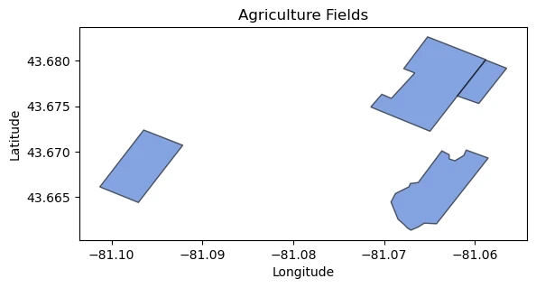
To order data, you need to provide areas of interest. You can do this by uploading GeoJSON features to a feature collection either through Features Manager or the Features API. Here we will use the Features API.

geojson_data = {"type":"FeatureCollection","features":[{"type":"Feature","properties":{},"geometry":{"coordinates":[[[-81.07147945222945,43.67490435965843],[-81.06495615860527,43.67223547577635],[-81.05882821611033,43.680122637871705],[-81.06521972602458,43.682624391132805],[-81.06785540021637,43.67912190735805],[-81.06663640090248,43.67864536315142],[-81.06920618323896,43.67585750370887],[-81.07026045291556,43.67631024182887],[-81.07147945222945,43.67490435965843]]],"type":"Polygon"}},{"type":"Feature","properties":{},"geometry":{"coordinates":[[[-81.05958597244029,43.675285619095064],[-81.05652200119249,43.67916956157043],[-81.05882821611033,43.68007498441628],[-81.06195807921277,43.67611961566857],[-81.05958597244029,43.675285619095064]]],"type":"Polygon"}},{"type":"Feature","properties":{},"geometry":{"coordinates":[[[-81.10129289138283,43.666119496077926],[-81.09704630815027,43.66439999452453],[-81.0921587312212,43.670698153259366],[-81.09645873059603,43.67237883850956],[-81.10129289138283,43.666119496077926]]],"type":"Polygon"}},{"type":"Feature","properties":{},"geometry":{"coordinates":[[[-81.05854129903942,43.6692934112491],[-81.06097545527373,43.6701737628008],[-81.06124321245954,43.66957512515077],[-81.06221687495348,43.66899408877978],[-81.06282541401194,43.66918776819534],[-81.06284975557425,43.669663160473675],[-81.06365302713158,43.67008572822684],[-81.06625757430251,43.66659945528957],[-81.06713387054724,43.66649380749428],[-81.06725557835875,43.66614164683307],[-81.06876475522422,43.66538449441549],[-81.0692515864712,43.66445124690017],[-81.06847265647616,43.66254949007825],[-81.06783977585489,43.662003604307216],[-81.06742596929533,43.66158097965604],[-81.06706084585984,43.66135205672751],[-81.06628191586482,43.661686636097585],[-81.06557601055715,43.66212686926988],[-81.06423722462823,43.662056432179355],[-81.05854129903942,43.6692934112491]]],"type":"Polygon"}}]}

# You may also choose to use your own geojson file for your own field boundaries

# Convert the GeoJSON data into a GeoDataFrame
features = [shape(feature["geometry"]) for feature in geojson_data["features"]]
properties = [feature["properties"] for feature in geojson_data["features"]]
agriculture_fields = gpd.GeoDataFrame(properties, geometry=features)

# Plotting setup
fig, ax = plt.subplots()
agriculture_fields.plot(ax=ax, color='#3366cc', edgecolor='black', alpha=0.6)

# Customize plot appearance
ax.set_title("Agriculture Fields")
ax.set_xlabel("Longitude")
ax.set_ylabel("Latitude")

# Show plot
plt.show()

With your API key, you can connect the features API.

# Set up authentication
PL_API_KEY = os.getenv("PL_API_KEY")

# Set up Planet Features API base URL
URL = "https://api.planet.com/features/v0/ogc/my/collections"

# Set up the session
session = requests.Session()
session.auth = (PL_API_KEY, "")

Create a feature collection

Now, you will create a feature collection to store the uploaded features.

request = {
    "title" : "Agriculture Fields",
    "description" : "A collection of agriculture field boundaries."
}

# Send the POST request to the API stats endpoint
res = session.post(URL, json=request)

# Print response
p(res.json())

# let's save the collection-id to use later
feature_collection_id = res.json()["id"]

Output
    {
      "id": "agriculture-fields-JvVxVDr",
      "title": "Agriculture Fields",
      "description": "A collection of agriculture field boundaries.",
      "item_type": "feature",
      "links": [
        {
          "href": "https://api.planet.com/features/v0/ogc/my/collections/agriculture-fields-JvVxVDr",
          "rel": "self",
          "title": "This collection",
          "type": "application/json"
        },
        {
          "href": "https://api.planet.com/features/v0/ogc/my/collections/agriculture-fields-JvVxVDr/items",
          "rel": "features",
          "title": "Features",
          "type": "application/json"
        }
      ],
      "feature_count": 0,
      "area": null,
      "title_property": null,
      "description_property": null,
      "permissions": {
        "can_write": true,
        "shared": false,
        "is_owner": true
      },
      "ownership": {
        "owner_id": 359883,
        "org_id": 1
      }
    }

Upload features to collection

With a feature collection created, you can upload features to the collection.

feature_refs = []

# Loop through each feature in the FeatureCollection
for i, feature in enumerate(geojson_data["features"]):
    # Extract geometry from feature
    geo = feature["geometry"]

    # Build request data with unique ID and properties
    request = {
        "geometry": geo,
        "id": str(i + 1),  # Generate a unique ID for each feature, you can adjust this
        "properties": {
            "title": f"Feature-{i + 1}",  # Customize title as needed
            "description": f"Description for Feature-{i + 1}"  # Customize description as needed
        }
    }

    # Make the POST request
    res = session.post(f"{URL}/{feature_collection_id}/items", json=request)

    # Process response and get short reference
    short_ref = res.json()[0]  # Adjust depending on API response format

    # Print or store the short reference for later use
    print(f"Short reference for feature {i + 1}: {short_ref}")

    feature_refs.append(short_ref)

Output
    Short reference for feature 1: pl:features/my/agriculture-fields-JvVxVDr/1-0aLYrRg
    Short reference for feature 2: pl:features/my/agriculture-fields-JvVxVDr/2-mEW2XBg
    Short reference for feature 3: pl:features/my/agriculture-fields-JvVxVDr/3-gBNDYVg
    Short reference for feature 4: pl:features/my/agriculture-fields-JvVxVDr/4-o4wld7m

For each input feature, we now have a corresponding unique identifier, called a feature reference. You can use these feature references to create subscriptions which will deliver PlanetScope data to your imagery collections.

Create PlanetScope subscriptions

We will iterate over each feature in the feature collection and create a subscription for it. To do this, we will use the Planet Python SDK.

You will need to specifiy a start and end time, as well as the item and asset types you want to subscribe to. In this example, we will subscribe to PlanetScope 8-band imagery.

A delivery desintation is also required for subscriptions. In this example, data is delivered to an image collection on Planet Insights Platform. You can also deliver data to your own cloud storage destinations.

# Set up authentication
pl_api_key = os.getenv("PL_API_KEY")
auth = planet.Auth.from_key(pl_api_key)

# Set up variables for creating the subscriptions

# Define a start and end time
start_time = datetime(2024, 3, 1, tzinfo=timezone.utc)
end_time = datetime(2024, 11, 1, tzinfo=timezone.utc)

# Set a collection ID, or set it to None and the function will a create a new collection
collection_id = None # "insert-collection-id-for-pre-existing"

# List of subscriptions created
subscriptions = {}

async with planet.Session(auth=auth) as sess:

    cl = SubscriptionsClient(sess)

    #For each feature in our geojson feature collection
    for feature_ref in feature_refs:

        feature_collection_id = short_ref.split("/")[-2]
        feature_id = short_ref.split("/")[-1]

        # Create a name for the subscription
        subscription_name = f"{feature_collection_id}_{feature_id}_PlanetScope"

        # Build the subscription payload
        payload = planet.subscription_request.build_request(
            name=subscription_name,
            source=planet.subscription_request.catalog_source(
                start_time=start_time,
                end_time=end_time,
                item_types=["PSScene"],
                asset_types=["ortho_analytic_8b_sr", "ortho_analytic_8b_xml", "ortho_udm2"],
                geometry={
                    "type": "ref",
                    "content": feature_ref,
                },
            ),
            hosting=planet.subscription_request.sentinel_hub(collection_id=collection_id),
        )

        # Create the subscription
        results = await cl.create_subscription(payload)
        subscription_id = results["id"]
        subscriptions[feature_ref] = subscription_id
        print(f"Feature Reference: {feature_ref} -> Subscription ID: {subscription_id}")

        # If no collection ID is set, set the collection ID as the collection created for the first subscription that is created
        if not collection_id:
            results = await cl.get_subscription(subscription_id=subscriptions[0])
            collection_id = results["hosting"]["parameters"]["collection_id"]
            await asyncio.sleep(3) # delay so collection can be established

print(f"{len(subscriptions)} Subscriptions created. Data is being delivered to the following collection: {collection_id}")

Output
    Feature Reference: pl:features/my/agriculture-fields-JvVxVDr/1-0aLYrRg -> Subscription ID: 9242db6f-d325-4e4a-bfc2-be431025dd8d
    Feature Reference: pl:features/my/agriculture-fields-JvVxVDr/2-mEW2XBg -> Subscription ID: ef6c1d03-5965-4bfd-b4b4-4414f7dbe37b
    Feature Reference: pl:features/my/agriculture-fields-JvVxVDr/3-gBNDYVg -> Subscription ID: 9bc73504-d779-403e-b698-1fef8699c86b
    Feature Reference: pl:features/my/agriculture-fields-JvVxVDr/4-o4wld7m -> Subscription ID: 266d0642-14be-4c2b-9446-1900b79c6371
    4 Subscriptions created. Data is being delivered to the following collection: 65834003-ca52-41b9-b089-34a8fa4eb9c0

Check subscription statuses

You now have one feature per area of interest and one subscription for each feature. You can poll the Subscriptions API to get their statuses.

async with planet.Session(auth=auth) as sess:

    cl = SubscriptionsClient(sess)

    for feature_ref, subscription_id in list(subscriptions.items()):
        sub_details = await cl.get_subscription(subscription_id=subscription_id)
        subscription_status = sub_details["status"]
        print(f"({subscription_status}) Feature Reference: {feature_ref} -> Subscription ID: {subscription_id}")

Output
    (running) Feature Reference: pl:features/my/agriculture-fields-JvVxVDr/1-0aLYrRg -> Subscription ID: 9242db6f-d325-4e4a-bfc2-be431025dd8d
    (running) Feature Reference: pl:features/my/agriculture-fields-JvVxVDr/2-mEW2XBg -> Subscription ID: ef6c1d03-5965-4bfd-b4b4-4414f7dbe37b
    (running) Feature Reference: pl:features/my/agriculture-fields-JvVxVDr/3-gBNDYVg -> Subscription ID: 9bc73504-d779-403e-b698-1fef8699c86b
    (running) Feature Reference: pl:features/my/agriculture-fields-JvVxVDr/4-o4wld7m -> Subscription ID: 266d0642-14be-4c2b-9446-1900b79c6371

note

Delivering data will take several minutes - continue to check in on the status. As data is delivered, you can jump into the second section. Until data is delivered, the section section will not work.

Analyze data to create indices and statistics

Now that data has been delivered to an image collection, you can use the Statistical and Process APIs to analyze the PlanetScope imagery that was ordered.

You must first install and configure the sentinelhub-py package.

config = SHConfig()

if not config.sh_client_id or not config.sh_client_secret:
    print("No credentials found, please provide the OAuth client ID and secret.")
else:
    print("Connected")

Output

    Connected

The following code will fetch the features from the API, extract geometries and properties from the features, create a GeoDataFrame, and reproject it to EPSG:3857. It's optimal to use a projected coordinate system for inputs into these APIs when working with small areas. This allows you to specify a resolution at which to analyze the data in units of meters instead of degrees, which is useful for small areas.

# Fetch the features from the API
res = session.get(f"{URL}/{feature_collection_id}/items")
features = res.json()['features']

# Extract geometries and properties from features
geometries = [shape(feature["geometry"]) for feature in features]
properties = [feature["properties"] for feature in features]

# Create GeoDataFrame and reproject to EPSG:3857
agriculture_fields = gpd.GeoDataFrame(properties, geometry=geometries, crs="EPSG:4326")
agriculture_fields_3857 = agriculture_fields.to_crs(epsg=3857)

# Display the reprojected GeoDataFrame
agriculture_fields_3857

	title	description	pl:ref	pl:area	geometry
0	Feature-4	Description for Feature-4	pl:features/my/agriculture-fields-JvVxVDr/4-o4...	405934.196941	POLYGON ((-9023395.542 5414406.396, -9023666.5...
1	Feature-3	Description for Feature-3	pl:features/my/agriculture-fields-JvVxVDr/3-gB...	314480.137995	POLYGON ((-9028154.627 5413917.953, -9027681.9...
2	Feature-2	Description for Feature-2	pl:features/my/agriculture-fields-JvVxVDr/2-mE...	106278.548884	POLYGON ((-9023511.834 5415328.625, -9023170.7...
3	Feature-1	Description for Feature-1	pl:features/my/agriculture-fields-JvVxVDr/1-0a...	548812.596246	POLYGON ((-9024835.810 5415269.945, -9024109.6...

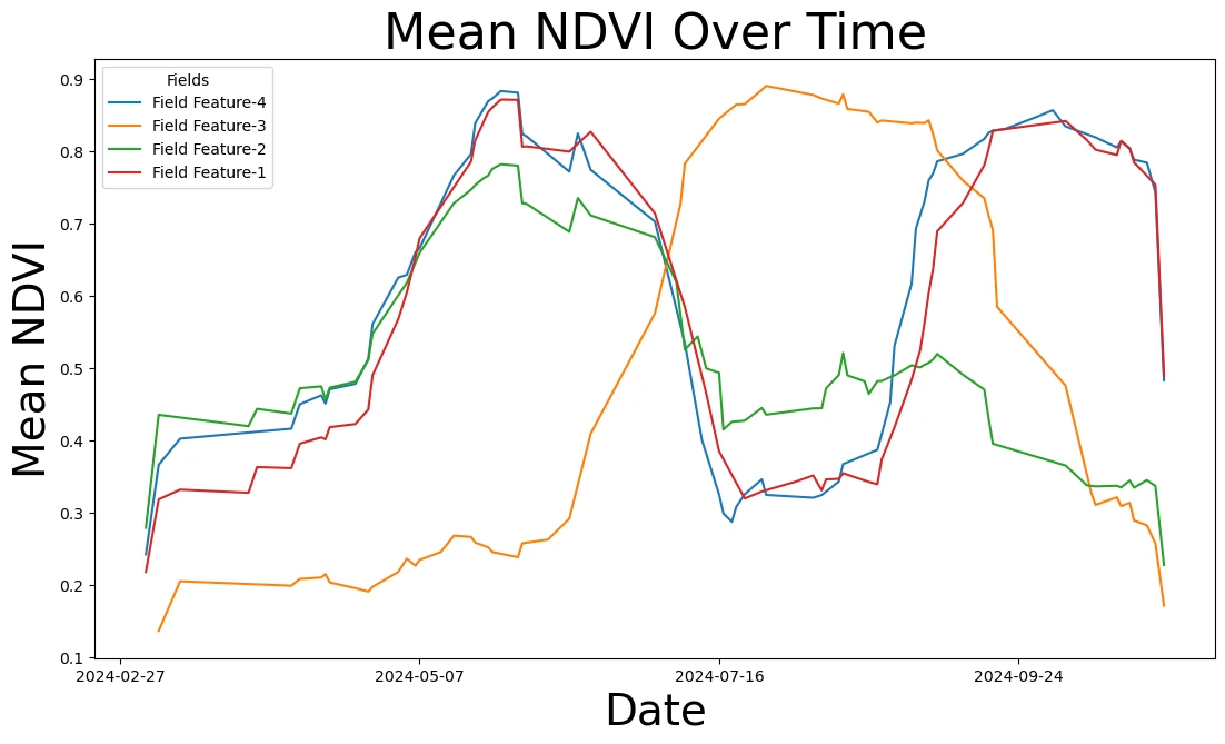
Create NDVI zonal statistics time series

For each area of interest, we can create a Statistical API request to calculate the NDVI zonal statistics time series. We will use the SentinelHubStatistical class from the sentinelhub-py package to create the requests.

You will need to provide inputs for

source imagery collection
time interval
spatial resolution
an evalscript
specification for aggregation intervals and histograms for statistics

image_collection = DataCollection.define_byoc(collection_id)

input_data = SentinelHubStatistical.input_data(image_collection)

# Set a time interval
time_interval = start_time.strftime('%Y-%m-%d'), end_time.strftime('%Y-%m-%d')

# Specify a resolution
resx = 3
resy = 3

# Provide an evalscript
evalscript = '''//VERSION=3

function setup() {
    return {
      input: [
        {
          bands: [
            "red",
            "nir",
            "dataMask",
            "clear"
          ]
        }
      ],
      output: [
        {
          id: "ndvi",
          bands: 2
        },
        {
          id: "dataMask",
          bands: 1
        }
      ]
    }
  }

  function evaluatePixel(samples) {

      let ndvi = (samples.nir-samples.red)/(samples.nir+samples.red);

      const indexVal = samples.dataMask === 1 ? ndvi : NaN;

      let id_default = colorBlend(ndvi,  [0.0, 0.5, 1.0],
        [
          [1,0,0, samples.dataMask * samples.clear],
          [1,1,0,samples.dataMask * samples.clear],
          [0.1,0.31,0,samples.dataMask * samples.clear],
        ])

        return {
          ndvi: [ndvi, samples.clear * samples.dataMask],
          dataMask: [samples.dataMask],
        };
  }'''

# Create the requests
aggregation = SentinelHubStatistical.aggregation(
    evalscript=evalscript, time_interval=time_interval, aggregation_interval="P1D", resolution=(resx, resy)
)

histogram_calculations = {"ndvi": {"histograms": {"default": {"nBins": 20, "lowEdge": -1.0, "highEdge": 1.0}}}}

# For each polygon field boundary, create a Statistical API request

agriculture_fields_3857 = agriculture_fields.to_crs(3857)

ndvi_requests = []

for geo_shape in agriculture_fields_3857.geometry.values:
    request = SentinelHubStatistical(
        aggregation=aggregation,
        input_data=[input_data],
        geometry=Geometry(geo_shape, crs=CRS(agriculture_fields_3857.crs)),
        calculations=histogram_calculations,
        config=config,
    )
    ndvi_requests.append(request)

print(f"{len(ndvi_requests)} Statistical API requests prepared")

Output

    4 Statistical API requests prepared

With the Statistical API requests prepared, you can download the data and create a time series of NDVI zonal statistics.

%%time

download_requests = [ndvi_request.download_list[0] for ndvi_request in ndvi_requests]

client = SentinelHubStatisticalDownloadClient(config=config)

ndvi_stats = client.download(download_requests)

print("{} Results from the Statistical API!".format(len(ndvi_requests)))

Output
    4 Results from the Statistical API!
    CPU times: total: 1.59 s
    Wall time: 41.8 s

Data is returned as json objects. We can normalize the data into a pandas DataFrame for further analysis.

ndvi_dfs = [pd.json_normalize(per_aoi_stats["data"]) for per_aoi_stats in ndvi_stats]

for df, feature_title in zip(ndvi_dfs, agriculture_fields.title):
    df["feature_title"] = feature_title

ndvi_df = pd.concat(ndvi_dfs)

# calculate date as day of the year for time integration
ndvi_df["day_of_year"] = ndvi_df.apply(lambda row: datetime.fromisoformat(row['interval.from'].rstrip('Z')).timetuple().tm_yday, axis=1)

# create a date field as a date data type
ndvi_df["date"] = pd.to_datetime(ndvi_df['interval.from']).dt.date

# delete and drop unused columns
del_cols = [i for i in list(ndvi_df) if i not in ["interval.from", "outputs.ndvi.bands.B0.stats.mean", "outputs.ndvi.bands.B1.stats.mean", "day_of_year", "feature_title", "date"]]
ndvi_df = ndvi_df.drop(columns=del_cols).rename(columns={'interval_from': 'date', 'outputs.ndvi.bands.B0.stats.mean': 'ndvi_mean', 'outputs.ndvi.bands.B1.stats.mean': 'clear', 'feature_title':'feature_title'})

# assign datatypes to float columns
ndvi_df['ndvi_mean'] = ndvi_df['ndvi_mean'].astype(float)
ndvi_df['clear'] = ndvi_df['clear'].astype(float)

ndvi_df

	interval.from	ndvi_mean	clear	feature_title	day_of_year	date
0	2024-03-01T00:00:00Z	0.014131	0.000000	Feature-4	61	2024-03-01
1	2024-03-04T00:00:00Z	0.354233	1.000000	Feature-4	64	2024-03-04
2	2024-03-07T00:00:00Z	0.374601	1.000000	Feature-4	67	2024-03-07
3	2024-03-08T00:00:00Z	0.102291	0.000000	Feature-4	68	2024-03-08
4	2024-03-10T00:00:00Z	0.027932	0.000000	Feature-4	70	2024-03-10
...	...	...	...	...	...	...
149	2024-10-24T00:00:00Z	0.741877	0.653461	Feature-1	298	2024-10-24
150	2024-10-26T00:00:00Z	0.771047	1.000000	Feature-1	300	2024-10-26
151	2024-10-27T00:00:00Z	0.118916	0.000000	Feature-1	301	2024-10-27
152	2024-10-28T00:00:00Z	0.697495	1.000000	Feature-1	302	2024-10-28
153	2024-10-30T00:00:00Z	0.472776	0.128951	Feature-1	304	2024-10-30

610 rows × 6 columns

# Suppress chained assignment warning for the specific line that requires it
pd.options.mode.chained_assignment = None

# Define the moving average function
def moving_average(x, w):
    return np.convolve(x, np.ones(w), 'same') / w

# Initialize plot
fig, ax = plt.subplots(figsize=(13, 7))

# Set up date formatting for x-axis
ax.xaxis.set_major_formatter(mdates.DateFormatter('%Y-%m-%d'))
ax.xaxis.set_major_locator(mdates.WeekdayLocator(interval=10))

# Plot each fields rolling average NDVI
for idx, feature_title in enumerate(agriculture_fields.title):
    series = ndvi_df[(ndvi_df["feature_title"] == feature_title) & (ndvi_df["clear"] >= 0.9)]

    # Calculate rolling average and assign directly
    series = series.copy()  # |Prevent chained assignment warning
    series["rolling_avg"] = moving_average(series["ndvi_mean"], 3)

    # Plot rolling average
    ax.plot(series["date"], series["rolling_avg"], label=f"Field {feature_title}", color=f"C{idx}")

# Set labels and title
ax.set_title('Mean NDVI Over Time', fontsize=32)
ax.set_ylabel("Mean NDVI", fontsize=28)
ax.set_xlabel("Date", fontsize=28)
ax.legend(title="Fields")

plt.show()

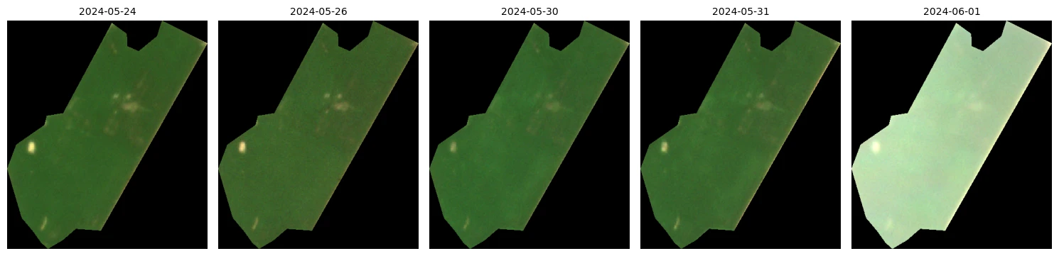
Create true color maps for cloud-free days

In this section, we will look at:

Requesting true color imagery over cloud free days
Performing multi-temporal analysis by caclulating the median NDVI from cloud-free images

To create our visualizations - let's start by selecting one field for the demonstration. In practice, you can batch these requests.

agriculture_field = agriculture_fields_3857.iloc[0]

print(agriculture_field)
agriculture_field["geometry"]

Output
    title                                                  Feature-4
    description                            Description for Feature-4
    pl:ref         pl:features/my/agriculture-fields-JvVxVDr/4-o4...
    pl:area                                            405934.196941
    geometry       POLYGON ((-9023395.541961536 5414406.39573724,...
    Name: 0, dtype: object

# Let's grab certain dates to visualize with the Processing API

# Subset the time series to one field where it's >90% clear
one_field = ndvi_df[(ndvi_df["feature_title"] == agriculture_field["title"]) & (ndvi_df["clear"].ge(0.9))]

# Find the date with the highest NDVI
peak_ndvi_date = one_field.loc[one_field['ndvi_mean'].idxmax(), 'date']

# Calculate a column for date difference from peak NDVI
one_field['date_diff'] = (one_field['date'] - peak_ndvi_date).abs()

# Find the 5 dates where we have clear imagery closest to the peak NDVI
one_field_sorted = one_field.sort_values(by='date_diff')

unique_acquisitions = one_field_sorted.head(5).sort_values(by="date")['date']

unique_acquisitions_list = unique_acquisitions.to_list()

unique_acquisitions_list

Output
    [datetime.date(2024, 5, 24),
     datetime.date(2024, 5, 26),
     datetime.date(2024, 5, 30),
     datetime.date(2024, 5, 31),
     datetime.date(2024, 6, 1)]

To visualize data in true color, you can use the following evalscript. This script will return true color imagery with a data mask to show cloud-free pixels.

true_color_evalscript = '''
//VERSION=3
//True Color

function setup() {
    return {
      input: ["blue", "green", "red", "dataMask", "clear"],
      output: { bands: 3 }
    };
  }

  function evaluatePixel(sample) {
    return [sample.red / 3000, sample.green / 3000, sample.blue / 3000, sample.dataMask*sample.clear];
  }
'''

And we can then loop through each timestamp and create a Process API requests for each date.

process_requests = []

time_difference = timedelta(hours=1)

for timestamp in unique_acquisitions_list:
    request = SentinelHubRequest(
        evalscript=true_color_evalscript,
        input_data=[
            SentinelHubRequest.input_data(
                data_collection=image_collection,
                time_interval=(timestamp, timestamp),
            )
        ],
        responses=[SentinelHubRequest.output_response("default", MimeType.PNG)],
        geometry=Geometry(agriculture_field["geometry"], crs=CRS("EPSG:3857")),
        resolution=(3, 3),
        config=config,
    )
    process_requests.append(request)

print("{} Process API requests prepared.".format(len(process_requests)))

Output

    5 Process API requests prepared.

%%time

client = SentinelHubDownloadClient(config=config)

download_requests = [request.download_list[0] for request in process_requests]

data = client.download(download_requests)

Output

    CPU times: total: 1.94 s
    Wall time: 2.45 s

ncols, nrows = 5, 1

fig, axis = plt.subplots(
    ncols=ncols, nrows=nrows, figsize=(15, 5),
    subplot_kw={"xticks": [], "yticks": [], "frame_on": False}
)

for idx, (image, timestamp) in enumerate(zip(data, unique_acquisitions_list)):
    ax = axis[idx]
    ax.imshow(np.clip(image * 2.5 / 255, 0, 1))
    ax.set_title(timestamp.isoformat(), fontsize=10)

plt.tight_layout()
plt.show()

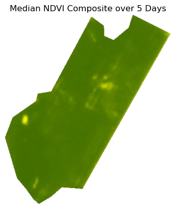
Create a median NDVI composite imagery with clouds removed

If you want to then take these multiple cloud free observations and create a composite for the median NDVI, you can do that with multitemporal analysis in the evalscript.

min_date = unique_acquisitions.min()
max_date = unique_acquisitions.max()

time_interval = min_date.strftime('%Y-%m-%d'), max_date.strftime('%Y-%m-%d')

print(time_interval)

Output

    ('2024-05-24', '2024-06-01')

The following evalscript will calculate the median NDVI from the cloud-free images.

median_ndvi_evalscript = '''
function setup() {
    return {
        input: ["red", "nir", "dataMask", "clear"],
        output: [{ id: "default", bands: 4 }],
        mosaicking: "ORBIT"  // Mosaicking method
    };
}

// Function to get the median value from an array
function getMedian(values) {
    values.sort((a, b) => a - b);
    const middle = Math.floor(values.length / 2);
    return values.length % 2 !== 0 ? values[middle] : (values[middle - 1] + values[middle]) / 2.0;
}

// Evaluate each pixel across all samples
function evaluatePixel(samples) {
    let ndviValues = [];

    for (let i = 0; i < samples.length; i++) {
        let sample = samples[i];
        // Include only cloud-free pixels (where clear and dataMask are both 1)
        if (sample.dataMask === 1 && sample.clear === 1) {
            let ndvi = index(sample.nir, sample.red);
            ndviValues.push(ndvi);
        }
    }

    // Calculate the median NDVI
    let medianNDVI = ndviValues.length > 0 ? getMedian(ndviValues) : null;

    return medianNDVI !== null
        ? colorBlend(medianNDVI,
            [0.0, 0.5, 1.0],
            [
                [1, 0, 0, samples[0].dataMask],
                [1, 1, 0, samples[0].dataMask],
                [0.1, 0.31, 0, samples[0].dataMask],
            ])
        : [0, 0, 0, 0];  // Transparent if no valid samples
}'''

request = SentinelHubRequest(
    evalscript=median_ndvi_evalscript,
    input_data=[
        SentinelHubRequest.input_data(
            data_collection=image_collection,
            time_interval=time_interval,
        )
    ],
    responses=[SentinelHubRequest.output_response("default", MimeType.PNG)],
    geometry=Geometry(agriculture_field["geometry"], crs=CRS("EPSG:3857")),
    resolution=(3, 3),
    config=config,
)

image = request.get_data()

plt.imshow(image[0])
plt.axis('off')
plt.title("Median NDVI Composite over 5 Days")
plt.show()

More resources

📖

API reference for Subscriptions API

Learn more about creating subscriptions.

📖

Evalscripts

Learn more about evalscripts to customize the data processing.

👩‍💻

Sentinel Hub Python SDK

Find more guides for using the Sentinel Hub Python SDK.

Prerequisites​

Set up your environment​

Upload areas of interest to feature collections​

Create a feature collection​

Upload features to collection​

Create PlanetScope subscriptions​

Check subscription statuses​

Analyze data to create indices and statistics​

Create NDVI zonal statistics time series​

Create true color maps for cloud-free days​

Create a median NDVI composite imagery with clouds removed​

More resources​

API reference for Subscriptions API

Evalscripts

Sentinel Hub Python SDK

Prerequisites

Set up your environment

Upload areas of interest to feature collections

Create a feature collection

Upload features to collection

Create PlanetScope subscriptions

Check subscription statuses

Analyze data to create indices and statistics

Create NDVI zonal statistics time series

Create true color maps for cloud-free days

Create a median NDVI composite imagery with clouds removed

More resources