Copy for LLM[View as Markdown](https://docs.planet.com/data/planetary-variables/soil-water-content/techspec/)
# Technical Specification
warning
Sales for Planet’s 20m and 100m Soil Water Content products have been discontinued. Active contracts remain fully supported through their remaining terms, and the core infrastructure will officially sunset in April 2028. Upon renewal, please contact your Account Executive to transition to our 1km product variant or explore other suitable alternatives for your specific use case.
## Overview
Soil water content (SWC) is an essential component of the hydrologic cycle. Also known as soil moisture, it refers to the water between the soil surface and the groundwater level in the unsaturated zone. This water is replenished by precipitation, irrigation, or capillary rise from deeper layers, and depleted by percolation, soil evaporation, and plant transpiration.
The Planet Soil Water Content product is based on the microwave radiation naturally emitted by the Earth. This passive microwave radiation is related to the water content in the soil and provides a direct measurement of water in the top layer of the soil. It is not sensitive to cloud cover and, therefore, allows for consistent, frequent, and global coverage.
The Planet patented algorithm enhances the spatial resolution of the passive microwave observations and the physical-based Land Parameter Retrieval Model retrieves the soil water content. Optical imagery from Sentinel-2 is used to further improve the spatial resolution.
Planet provides SWC data at 20, 100, and 1000 meter resolutions. With an archive spanning over 20 years, the data is consistent across time and space, boasting a strong correlation with ground data and accurately reflecting weather patterns. It is a cost-effective and low-effort alternative for measuring soil water content with physical sensors, making it suitable for many use cases like agriculture, water management, and insurance.
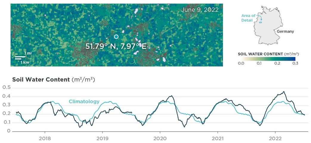
*Figure 1: Measurements of SWC near Ahlen, in North Rhine-Westphalia, Germany. The measurements of SWC of a single point are plotted over 5 years with the baseline climatology, showing how soil water content levels compare to the expected average for the area.*
## Product Specifications
*Table 1: SWC 20 m product specification*
| Data Resource | SWC 20 m |
| --------------------- | ------------------------------------------------------------------------------------------------------------------------------------ |
| Source ID | SWC-field\_V1.0\_20 |
| Satellites Used | AMSR-2, AMSR-E, SMAP, Sentinel-2 |
| Band | L, C and X-band |
| Version | 1.0 |
| Unit | m³/m³ |
| Sensing Depth | \~5 cm |
| Pixel Size | 20x20 m |
| Temporal Resolution | 267-364 observations/year |
| Overpass Time | 06:00 local solar time |
| Geographical Coverage | Global |
| Data Availability | 2018-01-01 - Present
Data Gaps:
2019-06-19 to 2019-07-24
2022-08-05 to 2022-09-24
2022-11-16 to 2022-11-18 |
*Table 2: SWC 100 m product specification*
| Data Resource | SWC 100 m L band | SWC 100 m C band | SWC 100 m X band |
| --------------------- | ------------------------------------------------------------------------------------------------------------------------------------ | ------------------------------------------------------------------------------------------------------- | ------------------------------------------------------------------------------------------------------- |
| Source ID | SWC-SMAP-L\_V2.0\_100 | SWC-AMSR2-C\_V2.0\_100 | SWC-AMSR2-X\_V2.0\_100 |
| Satellites Used | AMSR-2, SMAP, Sentinel-2 | AMSR-2, Sentinel-2 | AMSR-2, Sentinel-2 |
| Band | L band | C band | X band |
| Version | 2.0 | 2.0 | 2.0 |
| Unit | m³/m³ | m³/m³ | m³/m³ |
| Sensing Depth | \~5 cm | \~2 cm | \~1 cm |
| Pixel Size | 100x100 m | 100x100 m | 100x100 m |
| Temporal Resolution | 0° latitude: 137 to 183 observations per year
40° latitude: 183 to 228 observations per year | 0° latitude: 205 to 228 observations per year
40° latitude: 274 to 292 observations per year | 0° latitude: 205 to 228 observations per year
40° latitude: 274 to 292 observations per year |
| Overpass Time | 06:00 local solar time | 01:30 local solar time | 01:30 local solar time |
| Geographical Coverage | Global | Global | Global |
| Data Availability | 2017-07-01 - Present
Data Gaps:
2019-06-19 to 2019-07-24
2022-08-05 to 2022-09-24
2022-11-16 to 2022-11-18 | 2017-07-01 - Present | 2017-07-01 - Present |
| NRT latency (p90) | 72 hours | 48 hours | 48 hours |
| Archive latency | Within 30 days after creating a subscription | Within 30 days after creating a subscription | Within 30 days after creating a subscription |
*Table 3: SWC 1000 m product specification*
| Data Resource | SWC 1000 m L band | SWC 1000 m C band | SWC 1000 m X band |
| --------------------- | ------------------------------------------------------------------------------------------------------------------------------------ | ------------------------------------------------------------------------------------------------------- | --------------------------------------------------------------------------------------------------- |
| Source ID | SWC-SMAP-L\_V5.0\_1000 | SWC-AMSR2-C\_V5.0\_1000
(2012 - present)
SWC-AMSRE-C\_V5.0\_1000
(2002 - 2011) | SWC-AMSR2-X\_V5.0\_1000
(2012 - present)
SWC-AMSRE-X\_V5.0\_1000
(2002 - 2011) |
| Version | 5.0 | 5.0 | 5.0 |
| Unit | m³/m³ | m³/m³ | m³/m³ |
| Sensing Depth | \~5 cm | \~2 cm | \~1 cm |
| Pixel Size | 1000x1000 m | 1000x1000 m | 1000x1000 m |
| Temporal Resolution | 0° latitude: 137 to 183 observations per year
40° latitude: 183 to 228 observations per year | 0° latitude: 205 to 228 observations per year
40° latitude: 274 to 292 observations per year | 0° latitude: 205 to 228 obs/year
40° latitude: 274 to 292 obs/year |
| Overpass Time | 06:00 local solar time | 01:30 local solar time | 01:30 local solar time |
| Geographical Coverage | Global | Global | Global |
| Data Availability | 2015-04-01 - Present
Data Gaps:
2019-06-19 to 2019-07-24
2022-08-05 to 2022-09-24
2022-11-16 to 2022-11-18 | 2002-06-15 - Present
Data gap:
2011-10-04 to 2012-07-25 | 2002-06-15 - Present
Data gap:
2011-10-04 to 2012-07-25 |
| Satellites Used | AMSR-2, SMAP | AMSR-E, AMSR-2 | AMSR-E, AMSR-2 |
| NRT latency (p90) | 72 hours | 24 hours | 24 hours |
| Archive latency | Within 30 days after creating a subscription | Within 30 days after creating a subscription | Within 30 days after creating a subscription |
The sensing depth described in the table is an estimation of the average condition. Several studies (For example, [Schmugge et al., 1986](https://ieeexplore.ieee.org/abstract/document/4072415); [Wang et al., 1987](https://ieeexplore.ieee.org/document/4072692); [Owe et al., 1998](https://agupubs.onlinelibrary.wiley.com/doi/abs/10.1029/98WR01469)) have shown that microwave-based soil water content penetration depth depends on the soil water content conditions and frequency. At 1.41 GHz the penetration depth varies from approximately 10 cm to 1 m for soil conditions ranging from saturated to dry, whereas at 10.7 GHz the penetration depth varies from less than a few mm to a little over 2 cm for similar conditions. Thus, the drier the soil, the deeper the sampling depth.
## Asset Properties
Assets differ between field-based and tile-based data resources:
* **SWC 20 m (field-based)**: Each observation is delivered as a single-band asset with metadata embedded in the GeoTIFF.
* **SWC 100 m and SWC 1000 m (tile-based)**: Each observation is delivered as a SWC data asset (`*swc.tif`) with metadata provided in a separate quality flag asset (`*swc-qf.tif`).
*Table 4: Asset properties of SWC 20 m data resources*
| Asset Name | Band Name | Unit | Type | Typical Range | No Data Value | Scale | Format |
| ---------- | --------- | ----- | ------ | ------------- | ------------- | ----- | ------- |
| swc | Band 1 | m3/m3 | UINT16 | 0 - 1 | 65535 | 0.001 | GeoTIFF |
*Table 5: Asset properties of SWC 100 m and SWC 1000 m data resources*
| Asset Name | Band Name | Unit | Type | Typical Range | No Data Value | Scale | Format |
| ---------- | --------- | -------- | ------ | ------------- | ------------- | ----- | ------- |
| swc | Band 1 | m3/m3 | UINT16 | 0 - 1 | 65535 | 0.001 | GeoTIFF |
| swc | Band 2 | m3/m3 | UINT16 | 0 - 1 | 65535 | 0.001 | GeoTIFF |
| swc-qf | Band 1 | unitless | UINT16 | NA | 0 | 1 | GeoTIFF |
## Methodology
### Passive Microwaves and Downscaling Method
The Planet Soil Water Content data is derived from satellite sensors that measure passive microwave radiation. Passive microwave technology detects natural microwave emissions from the Earth's surface, which are sensitive to soil water content.
Using a patented algorithm ([US10643098](https://patentimages.storage.googleapis.com/1a/6f/1c/8cf51399ee7eaa/US10643098.pdf), [EP3469516B1](https://patentimages.storage.googleapis.com/f1/6c/0b/55cad50731d3e0/EP3469516B1.pdf)), we combine and downscale observations from multiple satellite constellation to a spatial resolution of 1000 m. We create footprints based on the footprint center, microwave frequency, incidence angle, azimuth angle, and footprint size, and then disaggregate them into equal interval ellipses using an internal Gaussian distribution. Within these ellipse-shaped footprints, the center contributes more to the observed values than the edges. By using fixed values for water bodies and filtering out influences such as radio frequency interference (RFI), we ensure accurate brightness temperatures.
### Enhancements Using Optical Data
The microwave observations are further downscaled to a spatial resolution of 100 m based on the Normalized Difference Shortwave Infrared (NDSWIR) index. This index is constructed from Near-Infrared (NIR) and Shortwave Infrared (SWIR) bands of Sentinel-2, namely B08 (842 nm) and B11 (1610 nm).
Several studies ([Lobell & Asner 2002](https://doi.org/10.2136/sssaj2002.7220), [Fensholt and Sandholt 2003](https://www.sciencedirect.com/science/article/abs/pii/S0034425703001895), [Sadeghi et al. 2017](https://doi.org/10.1016/j.rse.2017.05.041), [Yue et al. 2019](https://doi.org/10.1016/j.isprsjprs.2019.06.012)) found that soil and plant water content significantly affect the reflection in the SWIR part of the spectrum. The NIR reflectance is influenced by the internal structure and dry matter content of leaves, but not by water content. By combining SWIR, which responds to water content, with NIR reflectance, we can more accurately retrieve water content from the reflectance data ([Gao 1996](https://doi.org/10.1016/S0034-4257\(96\)00067-3), [Ceccato et al. 2001](https://doi.org/10.1016/S0034-4257\(01\)00191-2)).
Planet produces a daily NDSWIR composite using a backward Gaussian weighted distribution. This composite integrates into the downscaling framework by attributing the weight of a brightness temperature to each pixel within the footprint. The output format remains similar to that of the downscaling algorithm without NDSWIR input.
The Sentinel-2 data is extracted from L2A - Bottom of the atmosphere (BOA) - reflectance in the [Sentinel-2 dataset documentation](https://docs.planet.com/data/public-data/copernicus/sentinel-2.md).
### Physical-Based Land Parameter Retrieval Model
The downscaled high resolution microwave observations are converted to soil water content using the physical-based Land Parameter Retrieval Model (LPRM) ([Owe et al. 2001](https://ieeexplore.ieee.org/abstract/document/942542); [Owe et al. 2008](https://agupubs.onlinelibrary.wiley.com/doi/full/10.1029/2007JF000769); [De Jeu et al. 2014](https://www.sciencedirect.com/science/article/abs/pii/S0022169414001139), [Van der Schalie et al., 2018](https://www.mdpi.com/2072-4292/10/1/107), [Van der Schalie et al., 2018](https://www.mdpi.com/2072-4292/13/13/2480)).
The basis for the retrieval relies on the fact that thermal radiation in the microwave region is emitted by all natural surfaces as a function of temperature. The propagation of microwaves through the soil is then dependent on the soil dielectric constant, which has an almost linear relationship with soil water content. Microwave technology is the only remote sensing method that measures a direct response to the absolute amount of water in the soil, with a sensing depth ranging from millimeters for 37 GHz to tens of cm for 1.4 GHz. Vegetation also contributes to the microwave signal by absorbing, reflecting, and emitting radiation.
LPRM solves the radiative transfer equation at different frequencies and polarizations to retrieve soil water content and is currently the baseline algorithm for the ESA Climate Change Initiative (CCI) soil moisture products ([Scanlon et al., 2021](https://esa-soilmoisture-cci.org/sites/default/files/documents/public/CCI%20SM%20v06.1%20documentation/ESA_CCI_SM_RD_D2.1_v2_ATBD_v06.1_issue_1.1.pdf)).
### Input Data
*Table 6: List of inputs for Soil Water Content production*
| Product | Description |
| ---------------------------------------------- | -------------------------------------------------------------------------------------------------------------------------------------------------------------------------------------------------------------------------------------------------------------------------------------------------------------------------------------------------------------------------------------------------------------------------------------------------------------------------------------------------------------------------------------------------------------------------------------------------------------------------------------------------------------------------------------------------- |
| Brightness Temperature L band | Soil Moisture Active Passive (SMAP) Level-1B Radiometer Half-Orbit Time-Ordered L band Brightness Temperatures, Version 5 (downloaded from [NSIDC](https://nsidc.org/data/spl1btb/) in HDF5 format). This Level-1B product provides calibrated estimates of time-ordered geolocated brightness temperatures at 1.41 GHz with a footprint size of 39x47 km. SMAP L band brightness temperatures are referenced to the Earth's surface with undesired and erroneous radiometric sources removed. Data has been available since April 2015 with a latency of 12 hours. Detailed information is available [here](https://nsidc.org/sites/default/files/smap_atbd_radiometerl1b_tb_rev-b_20150401.pdf). |
| Brightness Temperature X band | Advanced Microwave Scanning Radiometer for EOS (AMSR-E) and Advanced Microwave Scanning Radiometer 2 (AMSR-2) Level-1B Radiometer X band Brightness Temperatures (downloaded from [JAXA G-portal](https://gportal.jaxa.jp/gpr/?lang=en) in HDF5 format). This Level-1B product provides calibrated estimates of geolocated brightness temperatures at 10.7 GHz with a footprint size of 24x42 km. Data has been available from July 2002 to October 2011 (AMSR-E) and from June 2012 (AMSR-2) up to now with a latency of 12 hours. Detailed information is available [here](https://gportal.jaxa.jp/gpr/assets/mng_upload/GCOM-W/AMSR2_Level1_Product_Format_EN.pdf) |
| Brightness Temperature C band | AMSR-E and AMSR-2 Level-1B Radiometer C band Brightness Temperatures (downloaded from [JAXA G-portal](https://gportal.jaxa.jp/gpr/?lang=en) in HDF5 format). This Level-1B product provides calibrated estimates of geolocated brightness temperatures at 6.9 GHz with a footprint size of 35x62 km. Data has been available from July 2002 to October 2011 (AMSR-E) and from June 2012 (AMSR-2) up to now with a latency of 12 hours. Detailed information is available [here](https://gportal.jaxa.jp/gpr/assets/mng_upload/GCOM-W/AMSR2_Level1_Product_Format_EN.pdf). |
| Brightness Temperature Ka band | AMSR-E and AMSR-2 Level-1B Radiometer Ka band Brightness Temperatures (downloaded from [JAXA G-portal](https://gportal.jaxa.jp/gpr/?lang=en) in HDF5 format). This Level-1B product provides calibrated estimates of geolocated brightness temperatures at 36.5 GHz with a footprint size of 7x12 km. Data has been available from July 2002 to October 2011 (AMSR-E) and from June 2012 (AMSR-2) up to now with a latency of 12 hours. Detailed information is available [here](https://gportal.jaxa.jp/gpr/assets/mng_upload/GCOM-W/AMSR2_Level1_Product_Format_EN.pdf). |
| Brightness Temperature W band | AMSR-E and AMSR-2 Level-1B Radiometer W band Brightness Temperatures (downloaded from JAXA G-portal in HDF5 format). This Level-1B product provides calibrated estimates of geolocated brightness temperatures at 89 GHz with a footprint size of 3x5 km. Data has been available from July 2002 to October 2011 (AMSR-E) and from June 2012 (AMSR-2) up to now with a latency of 12 hours. Detailed information is available [here](https://gportal.jaxa.jp/gpr/assets/mng_upload/GCOM-W/AMSR2_Level1_Product_Format_EN.pdf). |
| Reflectances SWIR and NIR (for SWC 20 m/100 m) | Sentinel-2 Level-2A reflectance [data](https://docs.planet.com/data/public-data/copernicus/sentinel-2.md) for two bands: SWIR (shortwave infrared around 1610 nm) and NIR (near infrared around 842 nm). |
| Digital Elevation Model | Digital elevation model (DEM) static map resampled at 100 m based on the Copernicus DEM GLO-90 product covering the full global landmass of the time frame of data acquisition (2011-2015). Detailed information is available in the link. |
| Land Cover Map | Custom global land classification including permanent water bodies based on the Copernicus Global Surface Water Bodies product from PROBA-V. Detailed information is available [here](https://land.copernicus.eu/global/) |
| Soil Map | Soil property maps resampled at 100 m based on the SoilGrids product. SoilGrids was funded by the core funding of ISRIC with additional support from the EUH2020 CIRCASA project. Detailed information is available [here](https://www.isric.org/explore/soilgrids), |
## Data Quality
### Uncertainty
The accuracy of soil water content retrievals from passive microwave observations and in particular the performance of the Land Parameter Retrieval Model has been described widely in the scientific literature: it has been compared to ground stations, hydrological models, and other satellite-derived products (for example, [Van der Schalie et al., 2021](https://www.mdpi.com/2072-4292/13/13/2480); [Gruber et al., 2020](https://www.sciencedirect.com/science/article/pii/S0034425720301760); [Gevaert et al., 2018](https://hess.copernicus.org/articles/22/4605/2018/)).
The accuracy of the retrievals depends on the microwave frequency. L-band soil water content has the highest accuracy of approximately 0.04 m³/m³, which is comparable to the accuracy of ground sensors (for example, see [Ganjegunte et al., 2012](https://link.springer.com/article/10.1007/s13201-012-0032-7)). The accuracy of the C and X band based products is approximately 0.05 m³/m³. In addition, the accuracy is a direct function of the vegetation cover as demonstrated by [Van der Schalie et al., 2018](https://www.mdpi.com/2072-4292/10/1/107).
The X and C band based retrievals are most sensitive to the density of the vegetation cover and provide the most reliable values with short vegetation. L band retrievals perform well over the majority of land covers, with the exception of dense tropical rainforest.
### Validation
We have evaluated our SWC products by comparing them to carefully picked ground data stations across various land cover types. The Pearson correlation coefficient varied between 0.53 and 0.92, indicating strong relations with ground truth data. Figure 2 shows a comparison between SWC data and ground data.
You can read more about the results in [this white paper](https://planet.widen.net/s/drrxtldpwg).
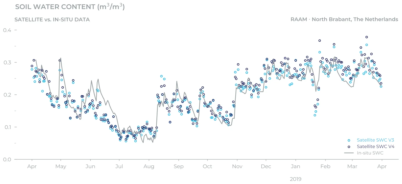
*Figure 2: Time series of the average of 9 stations of the RAAM network, the Netherlands.*
### Metadata
#### SWC 20 m
Metadata embedded in the GeoTIFF contains information about the quality of the observation. For example:
| Field | Type | Description | Example |
| ------------------- | ----------------- | --------------------------------------------------------------------------- | -------------------------------------------- |
| `PRODUCT_VERSION` | String | Version identifier for the product specification | `v1` |
| `SOFTWARE_VERSION` | String | Version of the fbsl software that generated the output | `0.4.1` |
| `INPUT_ASSETS` | String | Comma-separated list of input data sources used | `NDSWIR_STATS,NDSWIR_RASTER,KA_V_DESC_STATS` |
| `LAST_NDSWIR_DATE` | String (ISO date) | Date of the last NDSWIR (Sentinel-2) observation with full coverage | `2024-01-19` |
| `LAST_NDSWIR_COV` | String (fraction) | Coverage fraction of the last NDSWIR observation used | `0.85` (= 85% coverage) |
| `QUALITY` | String | Overall quality assessment: `HIGH` if valid coverage > 80%, otherwise `LOW` | `HIGH` or `LOW` |
| `FUSION` | String | Whether L-band fusion was applied | `YES` or `NO` |
| `DIVERGENCE_COV` | String (fraction) | Fraction of pixels where LPRM algorithm did not converge | `0.05` (= 5% divergence) |
| `QA_MDPI_LT_0_0001` | String (fraction) | Fraction of pixels with Modified Dual Polarization Index < 0.0001 | `0.12` (= 12% of pixels) |
| `QA_NO_COVERAGE` | String (fraction) | Fraction of pixels with no microwave coverage | `0.0` (= 0% missing) |
| `QA_FREEZING` | String (fraction) | Fraction of pixels flagged as freezing conditions | `0.0` (= 0% frozen) |
#### SWC 100 m and SWC 1000 m
Quality flag assets (`*swc-qf.tif`) provide metadata for each pixel using bitwise flags. Critical flags indicate unreliable data, with corresponding pixels in band 1 of the SWC asset (`*swc.tif`) set to the no data value. The replaced SWC value can be found in band 2 of the SWC asset. Non-critical flags indicate that the data can be used with caution, taking into account the flag description.
Critical and non-critical flags are described in the tables below. For more information on how to access the quality flag asset, check out [subscribing to planetary variables](https://docs.planet.com/develop/apis/subscriptions/sources.md).
*Table 7: Non-critical flags*
| Bit | Flag layer | Description |
| --- | ----------------------------- | ------------------------------------------------------------------------------------------------------------------------------------------------------------------------------------------------------------------------------------------- |
| 1 | Dense vegetation | The retrieved soil water content is less reliable over dense vegetation cover. |
| 2 | Low soil water content | The retrieved soil water content is lower than the estimated wilting point. |
| 3 | High soil water content | The retrieved soil water content is higher than the estimated porosity. |
| 4 | Possible severe precipitation | Part of the footprints touch an area flagged as severe precipitation. |
| 5 | Possible RFI | Footprints are contaminated for less than 25% with Radio Frequency Interference (RFI). RFI occurs when human-made transmitters emit in the same frequencies and thus disrupt the radiometer measurements of the natural microwave emission. |
| 7 | Possible frozen soil | The soil may be frozen. These are pixels with a soil temperature between -10°C and 0°C. |
*Table 8: Critical flags*
| Bit | Flag layer | Description |
| --- | ----------------------------------------- | ------------------------------------------------------------------------------------------------------------------------------------------------------------------------------------------------------------------------------------------- |
| 6 | Statistical outlier | The underlying footprint is considered a statistical outlier. |
| 8 | Frozen soil | The soil is frozen. Pixels with a soil temperature below -10°C. A conservative value of -10°C was chosen to avoid masking valid data. |
| 9 | Severe precipitation | Severe precipitation is detected. |
| 10 | Vegetation too dense | The vegetation cover is too dense for the algorithm to reliably retrieve soil water content. |
| 11 | No overpass | The satellite did not pass over. |
| 12 | RFI | Footprints are contaminated for more than 25% with Radio Frequency Interference (RFI). RFI occurs when human-made transmitters emit in the same frequencies and thus disrupt the radiometer measurements of the natural microwave emission. |
| 13 | Instrumental flaws | Unrealistic values due to instrumental flaws. If the brightness temperature at 36.5 GHz V produces values either over 400K or under 0.9 \* the water temperature, the data is considered as unrealistic and is removed. |
| 14 | Out of valid range | Soil water content values are outside the valid range, meaning under 0 m3/m3 or above 1 m3/m3. |
| 15 | Open water | Soil water content is not defined over water. |
| 16 | Brightness temperature residuals too high | The LPRM model could not find a soil water content value that is consistent with all provided input data. |
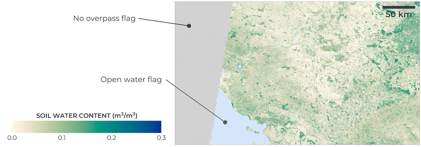
*Figure 3: An example of two quality flags for a region around Nantes, France. The image shows critical flags 'open water' and 'no overpass' overlaid on SWC 100 m.*
The following Python script converts a quality flag pixel value into a list of corresponding quality flags. Note that one pixel may have multiple flags applied to it.
```
# swc_quality_flags.py
import argparse
SWC_QUALITY_FLAGS = {
1: "Dense vegetation",
2: "Low soil water content",
3: "High soil water content",
4: "Possible severe precipitation",
5: "Possible RFI",
6: "Statistical outlier (critical flag)",
7: "Possible frozen soil",
8: "Frozen Soil (critical flag)",
9: "Severe precipitation (critical flag)",
10: "Vegetation too dense (critical flag)",
11: "No overpass (critical flag)",
12: "RFI (critical flag)",
13: "Instrumental flaws (critical flag)",
14: "Out of valid range (critical flag)",
15: "Open water (critical flag)",
16: "Brightness temperature residuals too high (critical flag)",
}
def convert_to_quality_flags(decimal_value: int) -> list[str]:
binary_string = format(decimal_value, "016b")
reversed_binary_string = binary_string[::-1]
return [
f"{i}. {SWC_QUALITY_FLAGS.get(i, 'Unused flag')}"
for i, bit in enumerate(reversed_binary_string, start=1) if bit == "1"
]
if __name__ == "__main__":
parser = argparse.ArgumentParser(description="Convert a decimal value to quality flags.")
parser.add_argument("decimal_value", type=int, help="The decimal value to convert.")
args = parser.parse_args()
flags = convert_to_quality_flags(args.decimal_value)
print(*flags, sep="\n")
```
that you can call as follows, using value `32770` as example:
```
> python swc_quality_flags.py 32770
2. Low soil water content
16. Brightness temperature residuals too high (critical flag)
```
## Other Limitations
The following are some key limitations that we have not flagged:
* SWC data should be considered unreliable over sloped terrain that is over 20 degrees. The microwave signal can be distorted by the angle of the slope, causing changes in the observed brightness temperature. This distortion leads to inaccuracies in the soil water content estimates because the algorithms assume a flat surface. Data usually shows up unrealistically dry.
* SWC data should be considered unreliable over urban areas. Human-made surfaces like concrete and asphalt have different microwave emissivity properties than natural soil. These surfaces can cause reflections and scattering of the microwave signal, leading to incorrect soil water content retrieval. Moreover, because urban areas have such a wide range of land cover types (asphalt, concrete, roofs, parks, gardens, etc) the average SWC value is not representative of any specific land cover type.
* Dynamic water bodies may cause unrealistic soil water content estimates. Water bodies influence the microwave observations and without proper mitigation they could result in unrealistic retrievals. Data around dynamic waterbodies can show up drier or wetter.
* Cloud cover hinders the optical observations by Sentinel-2 that are used for the SWC 100 m products. The downscaling can therefore only be updated when we obtain a cloud-free observation and the SWC data may suddenly increase or decrease after a long spell of no observations.
* False cloud/shadow detections may occur if surface conditions change very rapidly, during prolonged cloudiness, or over AOIs with significant terrain and shadowing. Significant effort has gone into developing automated techniques to differentiate between actual change and atmospheric contamination, but there may still be false detections.
* The SWC product integrates passive microwave data streams from multiple satellite missions. In rare instances where source data is completely unavailable, Planet cannot calculate SWC for that specific date. Once the 30-day reanalysis window closes, any such missing date in the subscription will be designated with a READY\_NO\_DATA status.
## Frequently Asked Questions
### There are three different bands for soil water content. What is a 'band' and which one should I use?
We use passive microwave observations to measure soil water content. A microwave signal is a light signal with a frequency that is much lower than the frequency of visible light. The lower the frequency of the passive microwaves, the more they tell us about what happens below the ground. A “band” refers to the frequency band we use to measure SWC. The lowest frequency band we deliver is the L-band (1.4 GHz), which is measured by the SMAP satellite. This measurement shows the water content in the top 5 cm of the soil. Other frequencies we deliver are the C-band (6.9 GHz), which shows the water content in the top 2 cm, and X-band (10.7 GHz), showing the top cm of the soil. The X-band and C-band measurements come from the AMSR-2 satellite.
For most use cases, L-band measurements are the best choice:
* They are representative of a deeper layer than the other bands.
* Vegetation on top of the soil has a much lower impact on the signal than for other bands.
* L-band observations are more sensitive to soil water content changes than the other bands: per unit change in soil water content, the microwave soil emission changes are stronger for L-band than for higher frequencies like C-band. This higher sensitivity leads to more accurate and precise SWC observations.
There are however some situations where the other bands are a better choice:
* Sometimes, radio signals emitted from the Earth interfere with the soil water content signals. We call this effect “radio frequency interference” (RFI). We filter for RFI, but sometimes the filter does not filter out everything, leading to strange SWC values. When this happens in the L-band for a specific location, use X-band or C-band.
* AMSR-2 provides the observations for X-band and C-band SWC. AMSR-2 data is available from 2012 onwards, and can be combined with data from its predecessor (AMSR-E) to compute long SWC time series, all the way back to 2002. When a customer wants to have a long time series, C-band and X-band data can go back to 2002. Our L-band product can provide SWC data from 2015 to present.
### What is the difference between the SWC 20 m, 100 m, and 1000 m products?
Our SWC 1000 m product is based on our patented disaggregation method where we make optimum use of the overlapping satellite footprints to refine the resolution from 36 km to 1 km. The SWC 100 m product also uses the NIR and SWIR band from Sentinel-2 to add more spatial constraints to our disaggregation method.
### Why does the SWC 1000 m product show a higher correlation with in-situ measurements than the SWC 100 m product?
Sometimes, customers compare our SWC products with in-situ measurements and find that the SWC 1000 m products perform better than the SWC 100 m products. This can be explained by the method used to enhance the spatial resolution. The SWC 1000 m product uses passive microwave observations, and has a temporal resolution of about 2 days, depending on the microwave band used and the latitude.
As a result, the SWC 1000 m product sees a lot of the temporal variations in SWC which are also caught by the in-situ sensor. For the enhanced-resolution products, we combine the passive microwave observations with infrared observations from the Sentinel-2 satellite. The infrared observations have a repeat cycle of about 5 days, depending on the latitude, but they cannot be made on cloudy days. The infrared data tell us how the soil water content is spatially divided within the coarser SWC 1000 m product and thus can accurately tell us which fields are relatively wet or dry, compared to the environment. However, the lower temporal resolution of the infrared data can cause the correlation coefficient to drop compared to the SWC 1000 m product. The enhanced-resolution product does get updated every time a new passive microwave observation comes in, but the temporal changes that result from the infrequent infrared observations can cause a degradation in the correlation.
Therefore, when a customer is interested mostly in the temporal changes, often the 1km products are the best choice. When they are interested in the spatial variations, the enhanced-resolution product can tell which areas are relatively dry or wet, compared to the environment.
### Is SWC a modeled product or an observation?
The brightness temperatures are direct observations by the satellite. These observations are used in a physical-based radiative transfer model to retrieve soil water content. However, considering the strong physical description of the radiative transfer model, scientists often refer to passive microwave soil water content as satellite-observed.
## Release notes
### June 1, 2025 - SWC 20 m v1.0
New Features:
* Increased spatial resolution for L-band product (25x)
* Field-based processing
* Metadata as raster-level tags in each geotiff (1-band raster delivered per observation)
### November 14, 2023 - SWC 1000 m V5.0 and SWC 100 m V2.0
New Features:
* Increased temporal resolution for L-band products
* Enhanced outlier detection capabilities
* Improved parameterization of the SWC retrieval model
* Refined water-body mask, enabling pixel size reduction from 1000m to 100m while maintaining consistent spatial support
* Updated quality flags for more accurate data assessment
warning
These new versions are not compatible with previous versions. Combining datasets from different versions may introduce offsets and scale discrepancies. We strongly advise against merging data from old and new versions.